


1 Introduction
Cavitation near boundaries generates large forces on surfaces in wall-normal and tangential directions. In particular, the stresses acting tangentially are important for cleaning and biological cell applications (Ohl et al. Reference Ohl, Arora, Ikink, De Jong, Versluis, Delius and Lohse2006b). Nonetheless, measuring the magnitude of these transient shear flows is non-trivial and only a few studies have taken up this challenge (e.g. Dijkink & Ohl (Reference Dijkink and Ohl2008) and recently Reuter & Mettin (Reference Reuter and Mettin2018)). In these studies, the geometry was a large boundary in a semi-infinite liquid domain. Yet, bubble dynamics in biological and cleaning applications occurs in more confined geometries such as in tubes and narrow constrictions. To understand how the confining geometry affects the interaction of the flow with the boundaries, we focus on bubbles and the shear generated in narrow gaps. Earlier, Gonzalez-Avila et al. (Reference Gonzalez-Avila, Klaseboer, Khoo and Ohl2011) reported on the collapse of a hemispherical bubble where the translational dynamics of the bubble during collapse depends on the ratio of the distance between the walls and the maximum horizontal extension of the bubble,  $\unicode[STIX]{x1D702}$. For sufficiently large values of
  $\unicode[STIX]{x1D702}$, the bubble collapses onto the same wall on which it was nucleated. Yet, when
  $\unicode[STIX]{x1D702}$ decreases the bubble splits during collapse and migrates to the opposite wall, where it may create considerable wall shear stress. This phenomenon allows for flow configurations where rigid surfaces can be exposed to strong tangential forces although the bubble is nucleated at some distance. This finding may allow for specific applications, i.e. cleaning applications in thin gaps such as in stacks of thin-film membranes or to induce forces on cells while preventing a physical contact of the bubble generator.
Besides the translatory movement of a cavitation bubble, numerical simulations conducted with an inviscid boundary element method revealed that the velocity of the jet formed within two walls is significantly larger as compared to a semi-infinite geometry (Krasovitski & Kimmel Reference Krasovitski and Kimmel2001; Gonzalez-Avila et al. Reference Gonzalez-Avila, Klaseboer, Khoo and Ohl2011). This suggests that the wall shear stresses are enhanced in a thin gap with important implications for confined cavitation bubble dynamics. To test this hypothesis we record the bubble dynamics of laser-induced cavitation bubbles at up to 500 kfps to resolve the evolution of a bubble’s shape as it approaches its minimum volume. We also report results from computational fluid dynamics simulations taking into account both liquid viscosity and surface tension and compare the bubble dynamics with experiments. Finally, we demonstrate applications of the flows for particulate removal and drug delivery into biological cells.
2 Experimental set-up
2.1 Experimental equipment
A schematic representation of the test section is shown in figure 1(a). The cavitation bubble is produced with a Q-switched Nd:YAG laser (Litron LPY, 532 nm wavelength, 6 ns pulse duration, 150 mJ maximum energy and 1.1 mm laser beam diameter). The laser beam is expanded, collimated and focused inside an acrylic cuvette with a  $\times 10$ microscope objective (Olympus UPlanFL N 0.30 NA). The test section has a glass window where the laser beam is introduced. The second wall is also made of glass and is parallel to the glass window. Both the test section and the upper wall are attached to a three-axis stage to control their absolute and relative position to within
  $\pm 10~\unicode[STIX]{x03BC}\text{m}$. To record the bubble dynamics between the parallel plates we use a high-speed camera (Shimadzu Hypervision, 1 Mfps maximum). The camera is coupled to a bellows focusing attachment (Nikon, model PB-6) and a 60 mm macro lens (Nikor) at full magnification. This arrangement results in a resolution of
  $20~\unicode[STIX]{x03BC}\text{m}$ per pixel. The scene was illuminated with diffused light from a flashlight (Sunpak 3075G, 4.4 ms pulse duration). Each test starts when a pulse delay generator (Quantum, 9520 series) triggers the laser, the camera and the flashlight. The maximum size attained by the bubbles in the horizontal direction,
  $R_{x}$, is
  $840\pm 60~\unicode[STIX]{x03BC}\text{m}$ (average of 30 tests). For demonstrating the applications of particle removal and cell membrane poration, a simpler method to generate cavitation bubbles was used. Spark-induced bubbles are induced by a high-voltage discharge (see Avila, Song & Ohl Reference Avila, Song and Ohl2015). The electrodes are etched on copper-plated printed circuit boards.
To evaluate the bubble dynamics and the spatial distribution of the wall shear stress, we use two dimensionless parameters: the non-dimensional channel height,  $\unicode[STIX]{x1D702}=H/R_{x}$, and the standoff parameter,
  $\unicode[STIX]{x1D6FE}=\unicode[STIX]{x1D6FF}/R_{eq}$, as depicted in figure 1(b). There,
  $H$ is the distance between the walls,
  $\unicode[STIX]{x1D6FF}$ is the distance between the bubble inception location and the wall and
  $R_{eq}$ is the radius of a spherical bubble with the same volume as a hemispherical bubble at maximum expansion with radius
  $R_{x}$. Using pulsed lasers to induce bubbles, the beam must be focused slightly above the glass substrate to avoid damage to the boundary. A safe distance used in this work is
  $\unicode[STIX]{x1D6FE}=0.46\pm 0.03$. In contrast, spark-induced bubbles are created on the substrate with considerably smaller
  $\unicode[STIX]{x1D6FE}\approx 0$.

Figure 1. (a) Schematic diagram of the experimental set-up. (b) Non-dimensional parameters.
2.2 Numerical simulations
The experimental results are compared to numerical simulations of the flow field by solving the compressible Navier–Stokes equation. The evolution of the gas–liquid interface is captured with the volume of fluid method using the finite volume framework in OpenFOAM. The volume of fluid simulations are carried out in an axisymmetric domain of 5 mm in radius and up to 2 mm in height. The initial grid consists of 100 cells in the radial direction, which is successively refined five times leading to a cell size of about  $1.5~\unicode[STIX]{x03BC}\text{m}$ where the bubble is located. To resolve the complex boundary-layer flow, the mesh is refined down to a size of
  ${\approx}50~\text{nm}$ near the walls. A no-slip boundary condition is used at both walls. The simulation starts with an initially spherical gas bubble of
  $50~\unicode[STIX]{x03BC}\text{m}$ in radius located
  $250~\unicode[STIX]{x03BC}\text{m}$ above the nucleated wall. The initial pressure of the spherical cavity was set to a high value. The model accounts for compressibility, surface tension and viscosity. The wall shear stress (Batchelor Reference Batchelor2000) of
 $$\begin{eqnarray}\unicode[STIX]{x1D749}=\unicode[STIX]{x1D707}\left.\frac{\unicode[STIX]{x2202}\boldsymbol{u}_{\boldsymbol{r}}}{\unicode[STIX]{x2202}y}\right|_{y=0}\end{eqnarray}$$
is obtained from the simulations through
 $$\begin{eqnarray}\unicode[STIX]{x1D749}\approx \unicode[STIX]{x1D707}\left.\frac{\boldsymbol{u}_{\boldsymbol{r}}(y)}{y}\right|_{y\leqslant \unicode[STIX]{x1D716}},\end{eqnarray}$$
 where  $\unicode[STIX]{x1D707}$ is the liquid dynamic viscosity,
  $\boldsymbol{u}_{\boldsymbol{r}}$ is the flow velocity parallel to the wall,
  $y$ is the distance to the boundary and the parameter
  $\unicode[STIX]{x1D716}$ defines the region inside the boundary layer where the shear rate is constant. To check the reliability of the numerical method, a simulation of a submerged jet is compared to the analytic solution derived by Glauert (Reference Glauert1956) and to the numerical results from Deshpande & Vaishnav (Reference Deshpande and Vaishnav1982). We obtain excellent agreement of the wall shear stress calculations once the region of constant shear rate is sufficiently resolved within the boundary layer; for details see Zeng et al. (Reference Zeng, Gonzalez-Avila, Dijkink, Koukouvinis, Gavaises and Ohl2018a). In the present studies, the wall shear stresses are obtained at a distance
  $y=0.1~\unicode[STIX]{x03BC}\text{m}$. The interested reader can find a detailed discussion of the model implementation in Zeng et al. (Reference Zeng, Gonzalez-Avila, Dijkink, Koukouvinis, Gavaises and Ohl2018a,Reference Zeng, Gonzalez-Avila, Ten Voorde and Ohlb).

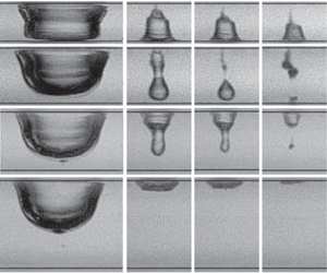
Figure 2. Selected examples of the bubble collapse for  $\unicode[STIX]{x1D702}=0.9,1.2,1.3$ and
  $1.9$. In all the sequences the bubble is nucleated on the upper wall. (a) Bubble migration to the lower wall;
  $\unicode[STIX]{x1D702}=0.9$,
  $R_{x}=840~\unicode[STIX]{x03BC}\text{m}$ and
  $H=740~\unicode[STIX]{x03BC}\text{m}$. (b) Bubble splits between the boundaries with the lower part collapsing on the lower wall;
  $\unicode[STIX]{x1D702}=1.2$,
  $R_{x}=880~\unicode[STIX]{x03BC}\text{m}$ and
  $H=1060~\unicode[STIX]{x03BC}\text{m}$. (c) Bubble splits between the walls leading to a neutral collapse;
  $\unicode[STIX]{x1D702}=1.3$,
  $R_{x}=890~\unicode[STIX]{x03BC}\text{m}$ and
  $H=1180~\unicode[STIX]{x03BC}\text{m}$. (d) Collapse onto the incepting upper wall;
  $\unicode[STIX]{x1D702}=1.9$,
  $R_{x}=900~\unicode[STIX]{x03BC}\text{m}$ and
  $H=1680~\unicode[STIX]{x03BC}\text{m}$. The black arrow at
  $t=166~\unicode[STIX]{x03BC}\text{s}$ points to the jet impacting on the nucleate wall. (e) Close-up of the fourth, fifth and sixth frames from the left shown in (a). The black arrows are an aid to the eye and point to the jet inside the bubble. Time is in microseconds; the length of the bar in upper left frame is
  $500~\unicode[STIX]{x03BC}\text{m}$.
3 Results
3.1 Overview
Figure 2(a–d) portrays the different collapse scenarios from selected images of the high-speed recordings with increasing distance,  $H$, between the walls. The black lines in each frame indicate the location of the upper and lower walls. In the sequences, the first image in each column depicts the shape of the bubble at maximum expansion. Interestingly, even at maximum expansion the bubble does not form a simple convex surface but presents circumferential undulations. These are likely the result of the oscillatory boundary-layer flow. As the bubble is approaching its maximum size, the ambient pressure is larger than the pressure inside the bubble. As a result, the liquid far from the bubble is accelerated back towards the axis of symmetry by this adverse pressure gradient. However, the bubble is still pushing the nearby liquid outwards and the expanding flow and the incoming flow collide. Due to the presence of the upper and lower walls, a downward flow from the upper wall and an upward flow from the lower wall are formed. These flows meet near the centre of the gap and form an annular jet flow towards the bubble where it forms a dimpled annular ring.
3.1.1 Bubble migration to the opposite wall
Starting with  $\unicode[STIX]{x1D702}=0.9$ (figure 2a), the bubble at maximum expansion seemingly touches both walls. While the bubble shape for times
  $t\geqslant 192~\unicode[STIX]{x03BC}\text{s}$ gives the impression that the liquid film at the lower wall has drained, the present imaging set-up does not allow a definite statement. During bubble shrinkage, the lower part of the bubble remains in close proximity to, or contact with, the lower wall, while the upper part of the bubble detaches from the upper wall at
  $t=196~\unicode[STIX]{x03BC}\text{s}$. Careful inspection reveals a tiny jet within the bubble at time
  $t=200~\unicode[STIX]{x03BC}\text{s}$ just above the lower wall. The three images in figure 2(e) portray the jet inside the collapsing bubble as it moves towards the opposite wall, indicated by the black arrows. From
  $t=196~\unicode[STIX]{x03BC}\text{s}$ to
  $t=202~\unicode[STIX]{x03BC}\text{s}$ the tip of the jet travels
  $480~\unicode[STIX]{x03BC}\text{m}$. This means that the jet impacts on the opposite wall with an average speed of at least
  $80~\text{m}~\text{s}^{-1}$. There exists an asymmetry between the time from bubble inception to maximum size (bubble expansion),
  $T_{exp}$, to bubble collapse, or the time from maximum size to minimum volume,
  $T_{col}$ of
  $T_{exp}=98~\unicode[STIX]{x03BC}\text{s}$ and
  $T_{col}=104~\unicode[STIX]{x03BC}\text{s}$, respectively. This may be explained with the formation of viscous boundary layers that delay the collapse.
Increasing  $\unicode[STIX]{x1D702}$ slightly from 0.9 to 1.2 changes the bubble dynamics as shown in figure 2(b). The lower part of the bubble remains round as it does not fully traverse to the lower boundary. The parts of the bubble closer to the boundaries shrink slower than the central part. As a result, the bubble splits at
  $t=194~\unicode[STIX]{x03BC}\text{s}$. The shape of the bubbles in the consecutive frames can be explained as the results of an annular jet rushing radially inwards from the centre
  $y=H/2$ and being deflected and transformed into an axial jet mostly into the downward direction. From the distance
  $L=440~\unicode[STIX]{x03BC}\text{m}$ (see figure 2b), we can estimate the averaged impact velocity of the jet onto the lower wall of
  $220~\text{m}~\text{s}^{-1}$. In contrast, the upper part of the bubble undergoes a mostly cylindrical collapse. Therefore, the present type of bubble collapse can be considered a migration scenario. In previous experiments (Gonzalez-Avila et al. Reference Gonzalez-Avila, Klaseboer, Khoo and Ohl2011), this value of
  $\unicode[STIX]{x1D702}$ could not be resolved due to a lower frame rate.
3.1.2 Collapse between the walls, neutral collapse
For  $\unicode[STIX]{x1D702}=1.3$, the lower part of the bubble during expansion no longer reaches the lower wall (figure 2c). The lower part obtains the shape of a cylinder with a rounded top and the upper part remains attached to the upper wall. The central part collapses first and thereby splits off from the upper attached bubble at
  $t=184~\unicode[STIX]{x03BC}\text{s}$. This scenario is named neutral collapse as the first collapse occurs near the centre of the gap. The upper part of the bubble impacts onto the upper wall with a speed of at least
  $130~\text{m}~\text{s}^{-1}$. Interestingly, the small change from
  $\unicode[STIX]{x1D702}=1.2$ to
  $\unicode[STIX]{x1D702}=1.3$ of figure 2(b) versus figure 2(c) greatly alters the collapse scenario and with it the forces acting on the walls.
3.1.3 Collapse onto the nucleation wall
In experiments we find that from  $\unicode[STIX]{x1D702}\geqslant 1.4$ the bubble collapses without splitting onto the upper wall, i.e. the wall closest to its nucleation location, resembling the dynamics of that observed from a single semi-infinite boundary. Figure 2(d) depicts the scenario for
  $\unicode[STIX]{x1D702}=1.9$. The jet impact velocity is
  $70~\text{m}~\text{s}^{-1}$.
3.2 Comparison with a computational fluid dynamics model

Figure 3. Comparison of experiment and simulation for a bubble of  $R_{x}=840~\unicode[STIX]{x03BC}\text{m}$ and
  $H=740~\unicode[STIX]{x03BC}\text{m}$ with
  $\unicode[STIX]{x1D702}=0.9$. The upper row of each panel depicts the high-speed images, the lower row the simulation results. Time is stated in microseconds; the length of the scale bar in the first frame is
  $500~\unicode[STIX]{x03BC}\text{m}$.
Before we report the wall shear stresses using a computational fluid dynamics model, we evaluate the ability of the model to describe the bubble dynamics between two walls. A comparison between the high-speed images and the simulated results for a bubble of  $R_{x}=748~\unicode[STIX]{x03BC}\text{m}$ and
  $H=750~\unicode[STIX]{x03BC}\text{m}$ with
  $\unicode[STIX]{x1D702}=1.0$ is depicted in figure 3. At
  $t=0$ the simulated bubble expands from a small spherical volume with an initial pressure of 1300 bar located
  $250~\unicode[STIX]{x03BC}\text{m}$ from the top boundary. The shape of the bubble or plasma is not available as images from the camera are overexposed. Yet, despite this numerical simplification for the initial condition, a good agreement of the bubble shape is obtained already from
  $t=6~\unicode[STIX]{x03BC}\text{s}$. The bubbles in the experiment and the simulation reach their maximum size at
  $t\approx 100~\unicode[STIX]{x03BC}\text{s}$ with the shape of an upside-down hat. During the early stage of the collapse, the middle part of the bubble collapses faster than the other parts and an hourglass-shaped bubble is formed. From
  $t=160~\unicode[STIX]{x03BC}\text{s}$ the part closer to the upper wall shrinks faster and forms a jet directed to the opposite wall. The jet accelerates through the bubble and impacts onto the lower wall. This results in a strong radial shearing flow. As a consequence of the jet boundary interaction, a toroidal bubble is formed that reaches its minimum volume at
  $t=202~\unicode[STIX]{x03BC}\text{s}$. The overall bubble dynamics is nicely reproduced, which provides confidence that the simulations resolve with sufficient accuracy the flow from which the wall shear stress is determined.
3.3 Wall shear stress measurements from simulations
3.3.1 Bubble migration to the opposite wall

Figure 4. Wall shear stress for  $R_{x}=735~\unicode[STIX]{x03BC}\text{m}$,
  $H=750~\unicode[STIX]{x03BC}\text{m}$ and
  $\unicode[STIX]{x1D702}=1.02$ of (a) the upper wall where the bubble is nucleated and of (b) the lower wall. The solid black line depicts the bubble’s equivalent radius. The wall shear stress in pascals is colour-coded in
  $\log _{10}$, where positive (red) values represent flow along the positive radial direction and negative values (blue) that towards the axis of symmetry. (c–f) Highlighting the bubble shape in the time interval
  $192~\unicode[STIX]{x03BC}\text{s}\leqslant t\leqslant 198~\unicode[STIX]{x03BC}\text{s}$ revealing the jet formation. Also depicted are the instantaneous flow field and wall shear stress distribution on the upper and lower wall. The velocity magnitude of the flow is colour-coded and the arrows point in the flow direction. The plots above and below each panel show the wall shear stress along the radial direction.
Figure 4(a,b) presents the spatio-temporal wall shear stress map on both walls for a bubble of  $R_{x}=735~\unicode[STIX]{x03BC}\text{m}$ and
  $H=750~\unicode[STIX]{x03BC}\text{m}$, and thus
  $\unicode[STIX]{x1D702}=1.02$. To cover the large range of the shear stress
  $\unicode[STIX]{x1D70F}(t,x)$, its logarithm (base 10) is plotted colour-coded. The positive stress that directs away from the axis of symmetry is coloured in red, while the negative values are in blue for the stress towards the axis of symmetry. The shear stress maps offer insight into the complex boundary-layer flows. For example, the largest stresses occur approximately when the bubble reaches its minimum size at
  $t\approx 200~\unicode[STIX]{x03BC}\text{s}$ simultaneously on both walls, with
  ${\approx}20~\text{kPa}$ on the upper wall and
  ${\approx}200~\text{kPa}$ on the lower wall (arrows next to IVa and IVb). Notice that the peak shear stress can even reach up to 1000 kPa for a brief instant and shortly after jet impact onto the lower wall (figure 4e) for
  $t=196~\unicode[STIX]{x03BC}\text{s}$. On both walls the stress is positive during most of the expansion,
  $0<t<50~\unicode[STIX]{x03BC}\text{s}$, as the bubble is then a source generating a radial outflow. At the later stage of the expansion and the start of the bubble shrinkage, the wall regions far from the bubble change sign (regions IIIa and IIIb) due to the inflow of liquid, while the stress remains positive on the walls covered by the bubble. The arrows IIa and IIb point to the locations where the near-wall flow velocity changes sign, indicating an inward-moving stagnation ring sweeping on the surface. Additionally, a region with particularly low shear stress is found on the nucleated wall as indicated in figure 4(a) with label Ia. This region forms because the liquid ‘trapped’ between the solid wall and the bubble is almost stagnant once the bubble reaches its maximum expansion protecting the wall from high shear stresses. As the bubble proceeds to collapse, this stagnant area shrinks. On the opposite wall, figure 4(b), during collapse from
  $t\approx 195~\unicode[STIX]{x03BC}\text{s}$ high stresses start near the axis of symmetry and spread with a velocity of about
  $25~\text{m}~\text{s}^{-1}$ outwards. The origin of this high-stress region being the jet is revealed in the snapshots of the bubble (figure 4c,d). Before a jet is formed, the upper part of the bubble shrinks faster than the lower part (see figure 4c). The overall inflow of the liquid towards
  $r=0$ creates a negative wall shear stress on both walls, except for the region confined by the lower bubble wall where the liquid is trapped. There the wall shear stress remains positive. Negative peaks of the wall shear stress are located just outside the hourglass-shaped bubble with a maximum (absolute) value of
  ${\approx}10~\text{kPa}$ on the nucleating wall and
  ${\approx}2~\text{kPa}$ on the lower wall. Figure 4(d) depicts the moment of jet development caused by the stagnation pressure of the inward-rushing liquid close to the upper wall. The flow has reflected from
  $r=0$ which results in a reversal of the stress direction with a positive value of
  $\unicode[STIX]{x1D70F}\approx 30~\text{kPa}$. As the flow is now fed into the jet and therefore downwards, the stress decays quickly with time. In contrast, the jet accelerates and reaches approximately
  $200~\text{m}~\text{s}^{-1}$ when it impacts the lower wall (figure 4e). The wall shear stress amplitude induced by the spreading jet is
  ${\approx}1000~\text{kPa}$. This value is about an order of magnitude higher than that in the single-wall case (see Zeng et al. Reference Zeng, Gonzalez-Avila, Dijkink, Koukouvinis, Gavaises and Ohl2018a).
Interestingly, alternating positive and negative shear stress values are found in figure 4(f), and more prominently in region Vb of figure 4(b). The reason is the separation of the boundary-layer flow due to the adverse pressure gradient. That is caused by the radially and fast outward-spreading jet flow meeting the still inward-rushing flow. As a result of this, the boundary-layer flow lifts off the plate and forms a system of ring vortices. A more detailed analysis is given in Zeng et al. (Reference Zeng, Gonzalez-Avila, Dijkink, Koukouvinis, Gavaises and Ohl2018a).
3.3.2 Collapse between the walls, neutral collapse

Figure 5. Wall shear stress on both walls for  $\unicode[STIX]{x1D702}=1.3$. (a) Nucleated wall; (b) opposite wall; (c–f) jet formation. (g) Close-up of the velocity distribution near the upper wall shown in (d). (h) Close-up of the velocity distribution on the lower wall shown in (e).
By increasing the liquid gap height, the location of the collapse is shifted towards the nucleating wall. Figure 5(a,b) plots the spatio-temporal wall shear stress distribution for the case  $\unicode[STIX]{x1D702}=1.3$ where the bubble splits and the first collapse occurs between the two walls (neutral collapse). The map of the upper wall, shown in figure 5(a), is very similar to that of figure 4(a). Yet, figure 5(b) depicting the shear stress on the lower wall reveals qualitative differences starting from the maximum bubble size, i.e.
  $t>90~\unicode[STIX]{x03BC}\text{s}$. There, the bubble does not reach as close to the lower wall and therefore no stagnant liquid region is formed. During the collapse the sign of the wall shear stress changes as the boundary-layer flow follows the bulk flow direction. The moderate shear stresses of a few kilopascals on the lower and upper walls increase considerably once the bubble splits between
  $t=178~\unicode[STIX]{x03BC}\text{s}$ and
  $t=180~\unicode[STIX]{x03BC}\text{s}$ (see figure 5c,d). There, the radial inflow creates a stagnation pressure around the centre of the gap near
  $r=0$ and drives two jets, one flowing downwards resulting in wall shear stress of
  $\unicode[STIX]{x1D70F}\approx 200~\text{kPa}$ and one with even higher stress on the upper wall of
  $\unicode[STIX]{x1D70F}\approx 700~\text{kPa}$. A close-up of the velocity distribution when the jet impacts and spreads on the upper and lower walls can be seen in figures 5(g) and 5(h), respectively.

Figure 6. Wall shear stress on both walls for  $\unicode[STIX]{x1D702}=2.0$. (a) Nucleated wall; (b) opposite wall; (c–f) jet formation.
3.3.3 Collapse onto the nucleation wall
On increasing the distance between the plates to 1.5 mm we obtain the bubble collapsing onto the nucleating wall. Figure 6(a,b) portrays the wall shear stress distribution for  $\unicode[STIX]{x1D702}=2.0$. In this case the opposite wall is effectively shielded from stresses with a maximum of only 200 Pa. The bubble dynamics and the stress distribution are similar to the case of a bubble collapsing near a single wall. However, due to the confinement of the opposite wall, the bubble collapses in a quasi-conical shape (Gonzalez-Avila et al. Reference Gonzalez-Avila, Klaseboer, Khoo and Ohl2011), forming a stronger jet than in the single-wall case. The maximum velocity of the jet is
  $120~\text{m}~\text{s}^{-1}$ and the maximum shear stress can reach
  ${\approx}150~\text{kPa}$. In this regime, at the nucleate wall stresses decay as the bubble dynamics proceeds, very similar to the shear stress distribution on the nucleate wall of the previous cases (see figures 4 and 5). However, on the opposite wall the transition from the positive to the negative shear stress is much sharper and up to three orders of magnitude lower than that occurring on the nucleate wall. The simulated results correspond to
  $\unicode[STIX]{x1D6FE}=0.3$. Also, in this regime, we found good agreement with the experimental bubble dynamics and the jet velocity (see figure 7). For this
  $\unicode[STIX]{x1D6FE}$ value the velocity of the jet is approximately three-fold larger than that measured for bubbles nucleated near a single wall,
  ${\approx}40~\text{m}~\text{s}^{-1}$ (Philipp & Lauterborn Reference Philipp and Lauterborn1998), and simulated,
  $38~\text{m}~\text{s}^{-1}$ (Lechner et al. Reference Lechner, Lauterborn, Koch and Mettin2019). We did not conduct experiments with smaller
  $\unicode[STIX]{x1D6FE}$ values. Therefore, we could not test an interesting regime that appears to produce viscosity-/curvature-induced jets that can reach
  ${\approx}1300~\text{m}~\text{s}^{-1}$ for
  $\unicode[STIX]{x1D6FE}\approx 0.1$, as shown by recently reported simulations (Lechner et al. Reference Lechner, Lauterborn, Koch and Mettin2019).
3.4 Jet velocity enhancement
It was already mentioned that the computed shear stress for small values of  $\unicode[STIX]{x1D702}$ is considerably larger as compared to a bubble in a semi-infinite geometry at the same value of
  $\unicode[STIX]{x1D6FE}$. We now discuss the jet velocities on impact obtained from the simulations and experiments as a function of the gap height
  $\unicode[STIX]{x1D702}$. It is important to note that the experimentally obtained impact velocity is a lower bound of the real velocity due to the inherent limitations of the high-speed cameras. There, the relative measurement error is caused by the limited temporal resolution
  $\unicode[STIX]{x0394}T$ and spatial resolution
  $\unicode[STIX]{x0394}L$; thus assuming independent variables we obtain
  $\unicode[STIX]{x0394}V_{jet}/V_{jet}=((\unicode[STIX]{x0394}L/L)^{2}+(\unicode[STIX]{x0394}T/T)^{2})^{1/2}$. Here
  $L$ is the measured distance the jet traverses during a time interval of
  $T$. The spatial uncertainty
  $\unicode[STIX]{x0394}L$ is estimated as
  $20~\unicode[STIX]{x03BC}\text{m}$ and the temporal uncertainty
  $\unicode[STIX]{x0394}T=1~\unicode[STIX]{x03BC}\text{s}$. For the fastest jets,
  $L=440~\unicode[STIX]{x03BC}\text{m}$ and
  $T=2~\unicode[STIX]{x03BC}\text{s}$. Unfortunately, the relative error can be considerable and for these jets reaches up to
  $\unicode[STIX]{x0394}V_{jet}/V_{jet}=50\,\%$. The results of all experiments performed are summarized in figure 7. The series shown represent the jet impact velocity. The filled symbols with error bars are the experimental values and the open symbols are the results from the simulation. Positive values of the impact velocity indicate an impact on the lower wall (opposite the nucleating wall). Overall, figure 7 demonstrates that the direction of the jet is a function of the value of
  $\unicode[STIX]{x1D702}$. Below
  $\unicode[STIX]{x1D702}\approx 1.2$ the bubble in the experiments and in the simulations collapses onto the lower wall; above
  $\unicode[STIX]{x1D702}\approx 1.4$ the bubble jets onto the upper wall. In the range
  $1.2\lesssim \unicode[STIX]{x1D702}\lesssim 1.4$, bubble splitting occurs where jets impact on both walls indicated by the two velocity values in the simulations. In the experiments, these two values are more difficult to measure and only the impact velocity on the upper wall can be extracted with confidence. Data indicated by arrows 2a–2d relate to the experiments shown in figure 2. Overall, we find qualitative agreement between the experiments and simulations of the three jetting regimes. The bubble-splitting regime has been narrowed down to
  $1.2\lesssim \unicode[STIX]{x1D702}\lesssim 1.4$ as compared to
  $1.0\lesssim \unicode[STIX]{x1D702}\lesssim 1.4$ in Gonzalez-Avila et al. (Reference Gonzalez-Avila, Klaseboer, Khoo and Ohl2011). We attribute this to the increased temporal resolution of the camera and the simulations incorporating boundary layers.
The experimentally observed fastest jets occur near and in the splitting regime with  $V_{jet}$ up to
  $220\pm 120~\text{m}~\text{s}^{-1}$ on the opposite wall, while the simulations predict
  $V_{jet}$ up to
  $280~\text{m}~\text{s}^{-1}$ at approximately the same value of
  $\unicode[STIX]{x1D702}$ of
  $1.2$. Considering the uncertainty in the measurements, the quantitative agreement between simulations and experiments is comfortable.

Figure 7. Experimental and simulated  $V_{jet}$ versus
  $\unicode[STIX]{x1D702}$. ‘Opp’ and ‘Nuc’ are the opposite and the nucleate walls, respectively.
For  $1.3\lesssim \unicode[STIX]{x1D702}\lesssim 1.4$, neutral collapse is observed. A sample of this collapse scenario is portrayed in figure 2(c). The images show that the bubble splits with one portion of the bubble collapsing between the walls and the other part collapsing onto the nucleate wall. At
  $t=184~\unicode[STIX]{x03BC}\text{s}$ the bubble has split and at
  $t=186~\unicode[STIX]{x03BC}\text{s}$ the bubble has already impacted on the nucleate wall; hence, the estimated jet velocity of
  $130~\text{m}~\text{s}^{-1}$ is a lower bound. The numerical results, for the same value of
  $\unicode[STIX]{x1D702}$, also portray a bubble that splits as it collapses. However, the portion of the bubble that collapses between the walls migrates and impacts on the opposite wall while the other portion of the bubble impacts on the nucleate wall. Notice that the numerical results show jets impacting on both walls for
  $1.3\leqslant \unicode[STIX]{x1D702}\leqslant 1.36$ (shaded region in figure 7). In this narrow range, the strength of the jet impacting on the opposite wall decreases with
  $\unicode[STIX]{x1D702}$, while the opposite trend is observed for the jets impacting on the nucleate wall. For
  $\unicode[STIX]{x1D702}=1.3$, the velocity of the jet on the opposite wall is
  $206~\text{m}~\text{s}^{-1}$ and that on the nucleated wall is
  $56~\text{m}~\text{s}^{-1}$. However, for
  $\unicode[STIX]{x1D702}=1.34$, the jet on the nucleated wall is faster than
  $191~\text{m}~\text{s}^{-1}$ and
  $94~\text{m}~\text{s}^{-1}$ on the opposite wall. The jet on the nucleate wall is the fastest at
  $210~\text{m}~\text{s}^{-1}$ for
  $\unicode[STIX]{x1D702}=1.36$. From
  $\unicode[STIX]{x1D702}\gtrsim 1.4$, experiments and simulations agree that the bubble collapses on the nucleate wall.

Figure 8. (a) The centroid of a cavitation bubble for different  $\unicode[STIX]{x1D702}$ values. (b) Close-up of the position of the bubble’s centre of mass as it approaches its minimum volume. The symbols in (b) are the same as in (a). The symbols represent experimental values; the grey line represents simulated values.
3.5 Centre of mass translation
Figure 8 portrays the displacement of the bubble’s centroid,  $C_{y}$, normalized by the liquid gap height,
  $H$, as a function of time. In the vertical axis
  $C_{y}/H=0$ and
  $C_{y}/H=1$ represent the nucleate and the opposite wall, respectively. The experimental centroids for the four collapse scenarios with
  $\unicode[STIX]{x1D6FE}=0.9$, 1.2, 1.3 and 1.9 are displayed in the figure. The simulated values of the
  $\unicode[STIX]{x1D6FE}$ = 0.9 trace are also added for comparison. In figure 8(a) two images accompany each trace. The first shows the bubble at maximum expansion and the second during bubble shrinkage. Figure 8(b) zooms into the last stage of collapse, 160
  ${\leqslant}t\leqslant 210~\unicode[STIX]{x03BC}\text{s}$. Again, selected frames of the bubble for each centroid movement are shown.

Figure 9. (a) Experimental set-up. (b) Electrodes used to test the particulate removal in a thin gap. (c) The three-dimensionally printed floating holder to test molecular uptake of RKO cells. (d–f) Schematic representation of bubble migration from the nucleate wall to the opposite wall. The red dots in (b–d) represent particles on a substrate or cells to be transfected as described in § 3.6.
All bubble centroids initially move downwards as the bubbles expand into the liquid gap. We see clear differences of the centroid motion between  $\unicode[STIX]{x1D6FE}=0.9$ (i.e. the bubble moves continuously towards the lower wall) and
  $\unicode[STIX]{x1D6FE}=1.3$ and 1.9 (i.e. the bubble translates back to the wall from where it was nucleated). For all cases, the centroid motion during the shrinkage is aligned with the direction of jetting. Comparing the measured with the simulated centroid motion,
  $\unicode[STIX]{x1D6FE}=0.9$, we see good agreement for the growth and early shrinkage. The last
  $15~\unicode[STIX]{x03BC}\text{s}$ of the experimental data are slower than predicted by the simulations. At the same time, we see some loss of axis symmetry in the simulations which are likely due to disturbances during nucleation of bubbles that grow during the collapse.
It is instructive to compare the two cases  $\unicode[STIX]{x1D6FE}=1.2$, where the bubble splits, and
  $\unicode[STIX]{x1D6FE}=1.3$, where the bubble jets onto the nucleating wall. Overall, their shapes and centroid locations are very similar, yet from about
  $t=150~\unicode[STIX]{x03BC}\text{s}$ their centroid motions start to deviate from each other. This hints to a competition between an annular flow splitting the bubble and the radial flow. On increasing the gap to
  $\unicode[STIX]{x1D6FE}=1.9$, the bubble grows and collapses onto the nucleate wall. Here, the centroid translates right after maximum expansion towards the closest wall.
3.6 Applications of bubble migration in a gap
Bubble generation utilizes high energy densities and temperatures that can be harmful to specific applications, e.g. when working with delicate biological cells or surfaces that are sensitive to high temperatures. We now present experiments carried out for  $0.6\leqslant \unicode[STIX]{x1D702}\leqslant 1.2$. This was done to utilize the small-
 $\unicode[STIX]{x1D702}$ regime of bubble migration that results in strong shear stress on the distant wall in the gap. Additionally, the bubbles are now generated with a high-voltage discharge in the liquid rather than a pulsed laser. This is much simpler, cheaper and easier to implement and therefore closer to practical application. The bubble generator utilizes a small spark gap powered by a piezoelectric high-voltage generator (see figure 9a). Details of the device are available in Avila et al. (Reference Avila, Song and Ohl2015). Two potential applications are now tested with experiments. The first experiment demonstrates the cleaning of a distant surface, and the second the transport of drugs through the plasma membrane of biological cells. Both experiments utilize an inverted microscope (Olympus IX71) with
  $\times 2$ and
  $\times 4$ magnifications and a high-speed camera (Photron SA-X2).

Figure 10. Bubble dynamics and resulting removal of particles from a substrate located at a distance  $h=600~\unicode[STIX]{x03BC}\text{m}$ from a spark gap. Maximum bubble radius
  $R_{x}=630\pm 50~\unicode[STIX]{x03BC}\text{m}$ and
  $\unicode[STIX]{x1D702}=1.0\pm 0.1$. The time is in microseconds.
3.6.1 Particle removal in a narrow gap
Here, an epoxy board with two copper electrodes where the bubbles are nucleated is attached to a three-axis stage (resolution of  $10~\unicode[STIX]{x03BC}\text{m}$) to control the gap height
  $H$, as shown in figure 9(b). To mimic particulate contamination, polystyrene particles (Thermo Scientific 2006A with a diameter of
  $6~\unicode[STIX]{x03BC}\text{m}$) are deposited onto the substrate by the evaporation of a suspended droplet at elevated temperatures. Thereby, a characteristic annular ring of weakly bonded particles resembling that from a coffee stain (Marín et al. Reference Marín, Gelderblom, Lohse and Snoeijer2011) is formed. Before an experiment is conducted, the upper wall is brought in contact with the lower wall to a region without particles. From this position, the distance
  $H$ is measured and an area with particles is chosen by moving the substrate laterally. Then a bubble is created and the event is recorded by the high-speed camera. We utilize bright-field and green fluorescence illumination as described in the supplementary material available at https://doi.org/10.1017/jfm.2019.938. The ring of particles is visible as dark patches in the first frame of figure 10 (bright-field illumination) and in figure 11 as bright objects (green fluorescence illumination). In the first frame of figure 10 the particles are imaged in focus. They are clustered within a thin annular region approximately
  $400~\unicode[STIX]{x03BC}\text{m}$ from the frame’s centre. Several larger clusters are visible within the annular ring. The electrodes can be seen as blurred horizontal lines separated by a gap. The distance between the electrodes and the substrate with the particles is
  $H\approx 600~\unicode[STIX]{x03BC}\text{m}$.
The consecutive frames in figure 10 depict the sequence of events resulting in the removal of these particles. The framing rate is 50 000 f.p.s. with an exposure time of  $1~\unicode[STIX]{x03BC}\text{s}$. The first row from frame
  $t=20~\unicode[STIX]{x03BC}\text{s}$ depicts the expansion of the cavitation bubble. It starts with the inception of the bubble from the electrodes. Until about
  $t=100~\unicode[STIX]{x03BC}\text{s}$ the bubble is imaged blurred due to the limited depth of focus. After nucleation the bubble expands and reaches its maximum size at
  $t=60~\unicode[STIX]{x03BC}\text{s}$ (
 $R_{x}=630~\unicode[STIX]{x03BC}\text{m}$,
  $\unicode[STIX]{x1D702}=1.0$).
The second row in figure 10 covering the time interval from  $t=100~\unicode[STIX]{x03BC}\text{s}$ to
  $t=160~\unicode[STIX]{x03BC}\text{s}$ portrays the shrinkage of the bubble. As the bubble migrates during this time towards the lower substrate it comes into focus. Between
  $t=160~\unicode[STIX]{x03BC}\text{s}$ and
  $t=180~\unicode[STIX]{x03BC}\text{s}$ a jet develops, pierces from the upper wall through the bubble, and starts to spread radially outward on the lower wall. The change of the bubble shape into a doughnut shape is visible at
  $t=180~\unicode[STIX]{x03BC}\text{s}$. The black arrow at
  $t=160~\unicode[STIX]{x03BC}\text{s}$ shows a cluster of particles that are detached and transported by the spreading jet in the consecutive frame
  $t=180~\unicode[STIX]{x03BC}\text{s}$. Between
  $t=200~\unicode[STIX]{x03BC}\text{s}$ and
  $t=220~\unicode[STIX]{x03BC}\text{s}$ the shear flow spreads and thereby removes more and more particles. While the first collapse occurs between
  $t=160~\unicode[STIX]{x03BC}\text{s}$ and
  $t=180~\unicode[STIX]{x03BC}\text{s}$ with an almost intact interface, the second collapse results in a disintegration of the torus into many small bubbles. These are leaving the field of view within 1 ms. Comparing the images before (
 $t=-20~\unicode[STIX]{x03BC}\text{s}$) and after (
 $t=1~\text{ms}$) reveals that most of the particles have been removed from the substrate.

Figure 11. Fluorescent polystyrene particles removed by a spark-generated cavitation bubble ( $h=720~\unicode[STIX]{x03BC}\text{m}$,
  $R_{x}=660\pm 110~\unicode[STIX]{x03BC}\text{m}$,
  $\unicode[STIX]{x1D702}=0.9\pm 0.2$). The event was captured at 36 kfps.
In figure 10 the bubble fragments and particles are difficult to distinguish from each other. To overcome this problem the experiments were repeated with fluorescent polystyrene particles (Thermo Scientific Fluoro-Max 36-4B with a diameter of  $15~\unicode[STIX]{x03BC}\text{m}$) similar to Ohl et al. (Reference Ohl, Arora, Dijkink, Janve and Lohse2006a). The particles are deposited again to the substrate and illuminated with a metal halide lamp (120Q Lumen Dynamics). Their larger diameter from the
  $6~\unicode[STIX]{x03BC}\text{m}$ in figure 10 to now
  $15~\unicode[STIX]{x03BC}\text{m}$ is needed to have enough fluorescence light emission, which together with the longer exposure time of
  $20~\unicode[STIX]{x03BC}\text{s}$ allows visualizing their motion with the high-speed camera, e.g. the nicely resolved bright ring in the first frame of figure 11. At the same time, the epifluorescent illumination provides contrast only to the particles. Therefore, while the particles are resolved, the bubble becomes invisible. To obtain an approximate diameter of the bubble, several runs were conducted with bright-field illumination and an average size of the created bubbles was obtained. The average size (over nine runs) of the bubbles is
  $R_{x}=660\pm 110~\unicode[STIX]{x03BC}\text{m}$ with
  $H=720~\unicode[STIX]{x03BC}\text{m}$ and
  $\unicode[STIX]{x1D702}=0.9\pm 0.2$, thus a situation comparable to that in figure 10. Figure 11 depicts the motion of the particles along the substrate before (
 $t=-28~\unicode[STIX]{x03BC}\text{s}$), during (
 $0\leqslant t\leqslant 222~\unicode[STIX]{x03BC}\text{s}$) and a long time after (
 $t=138~\text{ms}$) bubble generation.
The plasma generated by the spark discharge,  $t=0$ in figure 11, is visible as a bright region in the centre of the frame and increases the fluorescence emission of the particles. The particles translate during the expansion phase at
  $t=56~\unicode[STIX]{x03BC}\text{s}$ where they are dragged outwards. During bubble shrinkage, the inward flow drags the particles towards the centre (see arrows at
  $t=195~\unicode[STIX]{x03BC}\text{s}$). Interestingly, while the expansion of the bubble accelerates the particles purely radially, the inwards flow has a circumferential instability visible at time
  $t=195~\unicode[STIX]{x03BC}\text{s}$. During bubble collapse, the jet impacting on the substrate reverses the particle motion as indicated with the arrows at
  $t=222~\unicode[STIX]{x03BC}\text{s}$. This back-and-forth motion leads to complex boundary-layer flow dispersing the particles such that the initial annular ring shape is lost (see figure 11 at
  $t=138~\text{ms}$). Most of the particles have been removed from the field of view either by transporting them out of focus or out of the observation area by the residual flow.
3.6.2 Molecular transport into cells
Biological cells with a plasma membrane can be temporarily opened for the transport of large molecules through shear stress (Miller, Miller & Brayman Reference Miller, Miller and Brayman1996; Bao, Thrall & Miller Reference Bao, Thrall and Miller1997; Ng & Liu Reference Ng and Liu2002). The importance of the shear stress was demonstrated for laser-induced cavitation (Dijkink et al. Reference Dijkink, Le Gac, Nijhuis, van den Berg, Vermes, Poot and Ohl2007) and acoustic cavitation (Ohl et al. Reference Ohl, Arora, Ikink, De Jong, Versluis, Delius and Lohse2006b) when the bubble is considerably larger than the adherent cells. There, the cells are on a rigid substrate, i.e. the geometry resembles a semi-infinite liquid. The present experiments and simulations reveal that even higher shear stress can be generated within a thin gap. By placing the bubble generator at a suitable distance from the substrate with adherent cells, a gap is formed. A suitable distance is that while the bubble is created on one side of the gap, it jets towards the distant wall with the adherent cells. The advantage of this geometry is that the cells are not exposed to high temperatures and voltages during bubble generation. We designed a home-built holder that mounts a printed circuit board with a single copper electrode etched onto it. The copper string is cut in the middle with a high-power infrared laser to generate a separation gap of  ${\approx}30~\unicode[STIX]{x03BC}\text{m}$. This was done to avoid the variation in the separation between the electrodes produced by the etching process (Avila et al. Reference Avila, Song and Ohl2015). The separation between the electrodes remained constant for at least 30 cavitation events tested. The gap height
  $H$ formed by the printed circuit board and the substrate with the cells is adjusted by varying the length of the holder
  $h$ mounted on top of a six-well culture plate (see figure 9c). We study the effect of the non-dimensional gap height
  $\unicode[STIX]{x1D702}$ on the detachment region and drug uptake. We use adherent colon carcinoma (RKO) cells and two molecules to test for successful molecule delivery, namely the relatively small molecule calcein (628 Da) and a larger 10 000 Da fluorescent-labelled sugar molecule (FITC-Dextran). The cells were seeded in six-well plates (cat. no. 140675, Roskilde, Denmark) made of polystyrene including a surface treatment with Nunclon™ Delta. This cell-culture-treated surface is hydrophilic and facilitates cell attachment and growth. The protocol for cell preparation and handling is provided in the supplementary material. The cells must remain immersed in a culture medium (salt solution) during the experiment since it contains all the important minerals, salt and pH value to keep the cells alive. Before an experiment was conducted, we deposited a droplet of silicone oil (with a viscosity of 5 cSt) on the electrodes before submersing the bubble generator into liquid. The oil remains attached to the substrate that holds the electrodes and allows reaching electric field strengths sufficient to induce dielectric breakdown and successive bubble formation.
Figure 12 summarizes the results for three different gap heights  $\unicode[STIX]{x1D702}$: the four leftmost frames in each row show the bubble dynamics, the molecule uptake is in the fifth frame and the cell detachment in the sixth frame for
  $\unicode[STIX]{x1D702}=0.6$ (figure 12a),
  $\unicode[STIX]{x1D702}=1.0$ (figure 12b) and
  $\unicode[STIX]{x1D702}=1.2$ (figure 12c). The dimensional gap heights are increasing from
  $H=270\pm 30~\unicode[STIX]{x03BC}\text{m}$ to
  $420~\unicode[STIX]{x03BC}\text{m}$ to
  $500\pm 30~\unicode[STIX]{x03BC}\text{m}$ for figure 12(a–c). The toroidal bubble shape displayed in figure 12(a) at
  $t=126~\unicode[STIX]{x03BC}\text{s}$ and figure 12(b) at
  $t=119~\unicode[STIX]{x03BC}\text{s}$ is caused by the jet piercing through the bubble and impacting onto the substrate where the cells are located: the bubble migrates to the opposite wall. However, figure 12(c) portrays a bubble that either splits or collapses onto the nucleating wall. Interestingly, the size and shape of the torus are similar to the size and shape of the region where cells are detached (the vacated area in the rightmost frames of figure 12a,b). This is the region where we expect from the simulations that a brief but very intense wall shear stress is created, as can be seen in figure 4(e). This impulsive shear results in an immediate detachment of the cells. The cells further outside this region remain attached and can take up the non-membrane permeant dyes. This indicates that small holes have been opened in the membrane to allow diffusive transport into the cells.

Figure 12. Fluorescent uptake of calcein in RKO cells for various values of  $\unicode[STIX]{x1D702}$: (a)
  $\unicode[STIX]{x1D702}=0.6\pm 0.1$; (b)
  $\unicode[STIX]{x1D702}=1.0\pm 0.1$; (c)
  $\unicode[STIX]{x1D702}=1.2\pm 0.1$. From left to right, each row consists of four high-speed images of the bubble dynamics, a fluorescent image and a bright-field image of the cells. The scale bar is
  $500~\unicode[STIX]{x03BC}\text{m}$.
A magnified fluorescent image of the region with cell detachment and drug delivery is depicted in figure 13(a). Two circular regions are indicated with the white dashed lines. The inner circle approximates the distance to where the cells are detached,  $R_{in}$, while the outer circle is the limiting distance where fluorescent dye uptake took place,
  $R_{out}$. The ratio
  $\unicode[STIX]{x1D719}=R_{out}/R_{in}$ is a function of the non-dimensional gap height
  $\unicode[STIX]{x1D702}$. If the goal were to increase drug delivery with least detachment, this ratio should be maximized. Figure 13(b) depicts
  $\unicode[STIX]{x1D719}$ as a function of
  $\unicode[STIX]{x1D702}$. In the relatively narrow range
  $0.65\leqslant \unicode[STIX]{x1D702}\leqslant 0.72$, the largest ratio
  $\unicode[STIX]{x1D719}$ is found. An increase of this ratio is also found when increasing
  $\unicode[STIX]{x1D702}>1$. However, there the region of the uptake area is rather small (see figure 12c). It is worth noticing that the shear stress depends on the jet velocity and on the thickness of the liquid layer between the bubble and the boundary. The liquid layer affects the spreading velocity and the resulting boundary-layer structure. Generally, a higher velocity does not guarantee higher shear stress. However, in this particular application, it may be desirable to reduce the interaction of the jet with the cells on the substrate to prevent the detachment of the cells. While the jet impinges on the opposite wall for
  $\unicode[STIX]{x1D6FE}>1.4$, the shear created on the wall with the cells leads to a small amount of molecule uptake. We speculate that the flow created by pancake-like bubbles may be more suitable. For
  $\unicode[STIX]{x1D6FE}\sim 0.4$, the bubble expands and collapses between the two walls, and therefore the detachment and damage to the cells may be avoided (see figure 3a in Gonzalez-Avila et al. (Reference Gonzalez-Avila, Klaseboer, Khoo and Ohl2011)).

Figure 13. (a) Example fluorescent image of the region of jet impact and spreading. The central region (1) is depleted of cells, and cells between radii  $R_{in}$ and
  $R_{out}$ (region (2)) have taken up the dye calcein. No uptake is observed for region (3). (b) The relative uptake area
  $R_{out}/R_{in}$ as a function of the non-dimensional gap height
  $\unicode[STIX]{x1D702}$ for the two tested molecules calcein and FITC-Dextran.
4 Discussion
A cavitation bubble collapsing in the vicinity of a large (semi-infinite) rigid wall experiences a pressure gradient pointing away from the wall. This gradient accelerates liquid and focuses it through the shrinking and translating bubble towards the boundary. For sufficiently close distances, the liquid jet impacts perpendicular onto the rigid wall and spreads radially (Blake, Taib & Doherty Reference Blake, Taib and Doherty1986; Tomita & Shima Reference Tomita and Shima1986; Philipp & Lauterborn Reference Philipp and Lauterborn1998; Brujan et al. Reference Brujan, Noda, Ishigami, Ogasawara and Takahira2018; Lauterborn et al. Reference Lauterborn, Lechner, Koch and Mettin2018). However, for bubbles collapsing in more complex geometries, i.e. near a corner (Brujan et al. Reference Brujan, Noda, Ishigami, Ogasawara and Takahira2018; Tagawa & Peters Reference Tagawa and Peters2018), between two rigid boundaries (Chahine Reference Chahine1982; Kucherenko & Shamko Reference Kucherenko and Shamko1986; Han et al. Reference Han, Zhu, Guo, Liu and Ni2018; Quah et al. Reference Quah, Karri, Ohl, Klaseboer and Khoo2018), between a rigid boundary and an elastic wall (Horvat et al. Reference Horvat, Orthaber, Schille, Hartwig, Löschner, Vrečko and Petkovšek2018) or in the presence of more than two boundaries (Zwaan et al. Reference Zwaan, Le Gac, Tsuji and Ohl2007; Brujan, Takahira & Ogasawara Reference Brujan, Takahira and Ogasawara2019), the flow is greatly altered.
As an example, a bubble expanding and collapsing in the centre of a liquid gap forms an annular jet which splits the bubble into two parts. The annular jet focuses at the centre of the gap and splits into two jets flowing in opposite directions and towards the boundaries (Chahine Reference Chahine1982; Kucherenko & Shamko Reference Kucherenko and Shamko1986; Ishida et al. Reference Ishida, Nuntadusit, Kimoto, Nakagawa and Yamamoto2001; Han et al. Reference Han, Zhu, Guo, Liu and Ni2018; Quah et al. Reference Quah, Karri, Ohl, Klaseboer and Khoo2018).
Nucleating the bubble instead off-centre in the gap also results in the splitting of the bubble (Han et al. Reference Han, Zhu, Guo, Liu and Ni2018). A collapse scenario that is at first surprising is observed for bubbles created very close to one of the two walls. Then, there is a range of bubble sizes for which the bubble migrates to the opposite wall, i.e. away from the wall where it was nucleated (Gonzalez-Avila et al. Reference Gonzalez-Avila, Klaseboer, Khoo and Ohl2011).
It is worth noticing that we are able to reproduce the same collapse scenarios reported before (Gonzalez-Avila et al. Reference Gonzalez-Avila, Klaseboer, Khoo and Ohl2011) despite the differences in the bubble size and the inception location. The bubbles reported here are almost 10 times larger than those in our previous work and the energy used to nucleate these bubbles is almost three orders of magnitude larger. The bubble energy  $E_{b}$, or the work exerted by the bubble on the liquid to open a cavity of a certain volume against ambient pressure, can be estimated as
  $E_{b}=P_{a}V$, where
  $V$ is the maximum volume of the cavity and
  $P_{a}$ is the ambient pressure. In our previous work, we could create cavitation bubbles very close to one of the walls, thus
  $\unicode[STIX]{x1D6FE}\sim 0.2$. The bubble energy (for
  $100~\unicode[STIX]{x03BC}\text{m}$ radius bubbles) was approximately
  $0.2~\unicode[STIX]{x03BC}\text{J}$ and the laser energy
  $E_{l}\sim 2~\unicode[STIX]{x03BC}\text{J}$, assuming 10 % efficiency for well-focused nanosecond laser pulses (Vogel et al. Reference Vogel, Noack, Nahen, Theisen, Busch, Parlitz, Hammer, Noojin, Rockwell and Birngruber1999). In the present experiments, the estimated laser energy is
  $E_{l}\sim 1~\text{mJ}$ for
  $800~\unicode[STIX]{x03BC}\text{m}$ radius bubbles. With respect to the nucleation site, we could not nucleate bubbles very close to the substrate without causing damage to the glass. Due to the limited frame rate, only a lower bound for the velocity of the jets was provided. In addition, due to the limited temporal resolution, it was difficult to determine if the bubble split and collapsed on the opposite wall for 1.0
  ${<}\unicode[STIX]{x1D6FE}<1.2$ or if it migrated to the opposite wall without splitting as the bubble reached its minimum volume. In the present work, we are able to discuss these previously unresolved regimes.
The flows generated by cavitation bubbles in these more complex geometries are often assumed inviscid and modelled with potential flow, i.e. using the boundary element method (Ishida et al. Reference Ishida, Nuntadusit, Kimoto, Nakagawa and Yamamoto2001; Krasovitski & Kimmel Reference Krasovitski and Kimmel2001; Hsiao et al. Reference Hsiao, Choi, Singh, Chahine, Hay, Ilinskii, Zabolotskaya, Hamilton, Sankin and Yuan2013; Avila et al. Reference Avila, Song and Ohl2015; Tagawa & Peters Reference Tagawa and Peters2018; Brujan et al. Reference Brujan, Takahira and Ogasawara2019). Although ignoring the boundary layers, these simulations describe very well gross features of the flow such as the shape of the bubble, direction of the jet and motion of the bubble centroid. Yet, close to the rigid boundaries, the no-slip boundary condition demands viscosity to be taken into account (Popinet & Zaleski Reference Popinet and Zaleski2002; Mohammadzadeh, Li & Ohl Reference Mohammadzadeh, Li and Ohl2017; Koukouvinis et al. Reference Koukouvinis, Strotos, Zeng, Gonzalez-Avila, Theodorakakos, Gavaises and Ohl2018; Lauterborn et al. Reference Lauterborn, Lechner, Koch and Mettin2018; Zeng et al. Reference Zeng, Gonzalez-Avila, Dijkink, Koukouvinis, Gavaises and Ohl2018a; Lechner et al. Reference Lechner, Lauterborn, Koch and Mettin2019). Han et al. (Reference Han, Zhu, Guo, Liu and Ni2018) compared the bubble dynamics in a viscous liquid gap with simulations with a small set of parameters, but did not analyse the boundary layers. In the present work, we place our focus on the boundaries using experiments at high frame rates that have sufficient resolution for comparison with simulations. The wall shear stress in the present work is obtained from the simulations rather than physical measurements. At present, the experimental tools to measure reliably this quantity are not existent. Although a novel technique from Reuter & Mettin (Reference Reuter and Mettin2018) shows some promise, it involves a tedious point measurement and lacks a comparison with a well-known and calibrated flow. In contrast, we utilize the excellent agreements of the bubble shape and timing between experiments and simulations to assume that the simulations resolve the flow sufficiently well and measure the wall shear stress from the simulations. These simulations predict that the magnitude of the wall shear stress may reach up to 1000 kPa and last only for a couple of microseconds. This is about 100 times larger than the best present technique from Reuter & Mettin (Reference Reuter and Mettin2018) has resolved. The reason for these high wall shear stresses is the jet impact velocity and unsteadiness of the flow, e.g. for an  $\unicode[STIX]{x1D702}$ value of between 1.1 and 1.2 the jet speed reaches
  $220~\text{m}~\text{s}^{-1}$ (see figures 2b and 7). This averaged velocity is approximately two times larger than the jet speeds reported by Philipp & Lauterborn (Reference Philipp and Lauterborn1998) near a single boundary.
The interesting finding in the present study is that strong shear flow can be generated on a wall where bubble inception occurs at a distance. This is particularly attractive in cleaning applications and the manipulation of delicate cells. For both applications, the shear-generating device does not need to be in contact with the cells or the substrate to be cleaned, as was shown in §§ 3.6.1 and 3.6.2. We limit our discussion to cavitation bubbles in confined spaces that experience a series of oscillations before diffusing back into the liquid. In contrast, acoustically driven bubbles that sustain volume oscillations are also capable of exerting shear-force actuation and steady streaming. This topic has been the subject of significant experimental (Ahmed et al. Reference Ahmed, Mao, Juluri and Huang2009; Wang, Rallabandi & Hilgenfeldt Reference Wang, Rallabandi and Hilgenfeldt2013), numerical (Liu et al. Reference Liu, Yang, Pindera, Athavale and Grodzinski2002) and theoretical (Marmottant & Hilgenfeldt Reference Marmottant and Hilgenfeldt2003; Doinikov & Bouakaz Reference Doinikov and Bouakaz2010; Rallabandi, Wang & Hilgenfeldt Reference Rallabandi, Wang and Hilgenfeldt2014) work. There, the interest lies in its relevance for applications such as micromixing (Ahmed et al. Reference Ahmed, Mao, Juluri and Huang2009) and vortex traps (Lutz, Chen & Schwartz Reference Lutz, Chen and Schwartz2006), and for emerging applications that require a deeper understanding of bubble dynamics in confined spaces, i.e. in the vicinity of biological material. While we focus on transient bubble dynamics, the reader interested in periodic shear generation can refer to the above references, the work of Maisonhaute, Brookes & Compton (Reference Maisonhaute, Brookes and Compton2002a) and Maisonhaute et al. (Reference Maisonhaute, Prado, White and Compton2002b) and the reviews by Riley (Reference Riley2001) and Dollet, Marmottant & Garbin (Reference Dollet, Marmottant and Garbin2019).
Even looking at the shear generated on a single rigid boundary, we find a strong discrepancy between measured and simulated shear stresses. Experimentally, the hot-film-based technique of Dijkink & Ohl (Reference Dijkink and Ohl2008) and the electrochemical approach of Reuter & Mettin (Reference Reuter and Mettin2018) find a wall shear stress of the order of 3–6 kPa. The maximum sizes attained by the cavitation bubbles in these studies are  $750~\unicode[STIX]{x03BC}\text{m}$ and
  $425~\unicode[STIX]{x03BC}\text{m}$, respectively. This means that the mechanical effects of the bubbles in those studies are comparable to those reported here. Both experimental methods miss a proper calibration method with a laminar flow. In addition, their bandwidths are limited to a few hundred kilohertz while the rise time of the shear stress in the simulation is sub-microseconds. There is, however, one experimental study that estimates the shear stress from the measurement of the flow velocity and the thickness of the boundary layer in acoustic cavitation with even higher shear stress than that reported here. Maisonhaute et al. (Reference Maisonhaute, Brookes and Compton2002a) obtained a flow velocity of between
  $110$ and
  $220~\text{m}~\text{s}^{-1}$ at a distance of 40–80 nm from the wall. That results (Maisonhaute et al. Reference Maisonhaute, Prado, White and Compton2002b) in a wall shear stress of 2.5–5 MPa. The acoustically driven bubbles were hemispherical rather than spherical with a diameter ranging from
  ${\sim}15$–
 $800~\unicode[STIX]{x03BC}\text{m}$. Interestingly, the estimated stress values were obtained under steady flow conditions, and hence they represent a minimum value. The transient behaviour of the shear stress is likely higher, but it was unable to be resolved.
5 Conclusions
We have studied the bubble dynamics between two parallel plates when a bubble is nucleated close to one of the plates. Depending on the non-dimensional gap height, three distinct collapse scenarios are found with greatly different wall shear stress contributions to both boundaries, namely migration to the opposite wall, neutral collapse and collapse onto the nucleate wall. The confined geometry may result in much faster jets than for a single boundary, i.e.  $220~\text{m}~\text{s}^{-1}$ as compared to
  $100~\text{m}~\text{s}^{-1}$. The experimental results are complemented with computational fluid dynamics simulations that account for compressibility, viscosity and surface tension. The simulated bubble dynamics reproduces most of the features observed in experiments. Therefore, we have confidence that the calculated shear stresses of up to 1000 kPa are indeed occurring, yet only briefly and on a small spatial scale. These shear stresses are about an order of magnitude higher than those found for bubbles of similar size collapsing in a semi-infinite geometry (Zeng et al. Reference Zeng, Gonzalez-Avila, Dijkink, Koukouvinis, Gavaises and Ohl2018a). The results are presented with wall shear stress maps that provide a quick overview of the complex dynamics occurring. The observation that the bubble creates large shear on the boundary opposite to the nucleating boundary may open up possibilities for applications. Here, we discussed the cleaning of particles from a remote surface and the molecular transport into biological cells.
Acknowledgements
The authors are grateful to the anonymous reviewers for their valuable comments and suggestions.
Declaration of interests
The authors report no conflict of interest.
Supplementary material
Supplementary material is available at https://doi.org/10.1017/jfm.2019.938.


