Classical logic

The proposal that classical logic is the appropriate foundation for rationality in decision making essentially goes back to antiquity. Operationally, the way classical logic can be used to build a psychological model (for rational decision making) typically involves an assumption of a mental logic, that is a set of logical rules represented in the mind, such that any new problem can be cast into a form that can be resolved using some combination of these logical rules (e.g., Braine et al., Reference Braine, O’Brien, Noveck, Samuels, Lea, Fisch and Yang1995). For example, consider the Wason selection task (Wason, Reference Wason1968). Participants are presented with four cards, for example, A, B, 1, 2. They are given this rule “If there is a vowel on one side of a card, there has to be an even number on the other side.” They are told that it is not known whether the rule is correct or not and that their job is to attempt to test the rule, by flipping cards and examining the information on the other side of each card. Note, participants know that all cards with a letter will have a number on the other side and vice versa. For example, in flipping the A card, there may be a 1 or 2 on the other side, the former being inconsistent with the rule and the latter consistent with the rule. According to a mental logic account of reasoning, the problem will be translated into a suitable abstract form (e.g., an “if, then” rule with abstract premises) and then various heuristic principles will dictate how the available cards can be utilized for testing the rule.

There have been several variations of the Wason selection task (e.g., Evans, Reference Evans1991; Evans, Newstead, & Byrne, Reference Evans, Newstead and Byrne1991), but the typical pattern of results is this: Most participants select the A card; many participants select the 2 card, hardly any participants select the B card, and likewise for the 1 card. The selection of the A card is clearly appropriate, since on observing a 2 on the other side we have some confirmation of the rule, but on seeing a 1 the rule is definitely refuted. The 2 card has potential to confirm the rule if, on flipping it, we observe an A on the other side. But if instead we see a B, then there is not much we can say about the rule, since the rule tells us nothing about situations for which there is B on the card. The B card is clearly not very helpful, as the rule does not apply when we have a B card. However, the selection of the 1 card would make sense: if on flipping the 1 card we see an A, then (again) we have definite evidence that the rule is false. The non-selection of the 1 card is the key result from the Wason selection task; it is the result which challenged the assumption that humans are rational (if rationality is understood in terms of classical logic), at the time. Eventually this result has led to decision theorists abandoning the view that classical logic is an appropriate foundation for human rationality (with a degree of self-interest, we could note that this is clearly preferable to a conclusion that humans are irrational).

Why is the non-selection of the 1 card so problematic? Because the 1 (and A) cards are the only ones which offer the potential of definite falsification of the Wason rule and so, according to classical logic (plus a principle that definite conclusions are the most desirable ones), the only rational choices. Note, here there is a slight conflation between classical logic as a rational standard for human decision making and a prerogative to reach definite conclusions, but this is less problematic than it may look, since an approach to human reasoning based on classical logic is essentially one of deductive inference.

The results of the Wason selection task do not necessarily reveal an inconsistency with classical logic, either as a normative or a descriptive framework for human reasoning. From a descriptive point of view, it is possible that the mind embodies a rational, logical module, but that this module operates on representations which are heuristically derived and so may contain inaccurate information (cf. Evans et al., Reference Evans, Newstead and Byrne1991). Or it is possible that reasoning behavior arises from the operation of multiple processes, such as a normative, logical one and one based on heuristics and biases. It is possible that the latter process is engaged more readily under conditions of time pressure, concurrent cognitive loads, or plain lack of interest – all of these conditions potentially apply in the case of participants taking part in a Wason selection task experiment. Such so-called dual (or multiple) route models of human reasoning and decision making have been popular, exemplifying a general intuition of a more intuitive vs. a more analytic mode to thought (Elqayam & Evans, Reference Elqayam and Evans2013; Evans, Handley, Neilens, & Over, Reference Evans, Handley, Neilens and Over2007; Kahneman, Reference Kahneman2001; Sloman, Reference Sloman1996).

Despite these potential ways in which a view of human rationality and behavior based on classical logic could be salvaged, the overall verdict on classical logic has been diminishing interest. In modern discussions of reasoning and decision making, classical logic tends not to be considered as a viable proposal (though note there are instances of employing logic in other ways in cognitive explanation, e.g., to measure complexity of composite concepts, Feldman, Reference Feldman2000). Note, one further reason for this diminishing interest regarding classical logic is the growing realization that deductive rules, as exemplified in classical logic, are not suitable for human everyday inference (Chater & Oaksford, Reference Chater and Oaksford1993). In other words, it seems that it is rarely the case that we can derive monotonic, non-defeasible conclusions in everyday life reasoning situations, as we would be required to do following classical logic.

It is worth briefly mentioning an interesting theoretical variant of mental logic, involving so-called pragmatic reasoning schemas (Cheng & Holyoak, Reference Cheng and Holyoak1985). According to this view, there is no abstract mental logic regardless of content. Rather, there are privileged (how? Because of their importance in our lives) contexts, which benefit from context-specific (logical) rules. So, in this account, logical reasoning would be guided by e.g. obligation or permission schemas, corresponding to obligation or permission reasoning problems. We illustrate a permission schema with one of Cheng and Holyoak’s (Reference Cheng and Holyoak1985) demonstrations. Consider a postal system such that letters can be posted either sealed or unsealed, but the former have to carry a more expensive stamp than the latter. The given rationale for this rule is that sealed letters are often personal letters and therefore requiring higher postage for such letters would increase corresponding profit. Participants were presented with four stimuli, corresponding to letters, such that for two letters the front was shown (and so it could be determined whether the letter was sealed or not sealed) and for two other letters the back was shown (and so participants could see whether the cheaper or more expensive stamp was used). Participants were then asked whether the rule “if a letter is sealed, it needs to carry the more expensive stamp” was being followed by checking (turning over) some of the envelopes. Note, this is a permission situation because it concerns the circumstances under which one is permitted to use the cheaper stamp. Cheng and Holyoak’s (Reference Cheng and Holyoak1985) experiment is clearly analogous to the Wason selection task. However, unlike for the Wason selection task, results in this experiment showed close consistency with the prescription from classical logic (when the rationale for the postal rule was included, but not without the rationale; the result was replicated with different materials and rules). However, even when considering these pragmatic reasoning schemas, the assumed normative standard is classical logic. How can the correct selections in the Wason selection task be anything other the ones recommended by classical logic?

Classical probability theory and information theory

Anderson (Reference Anderson1990, Reference Anderson1991a, Reference Anderson1991b) advocated an influential view of rationality, according to which rationality is tantamount to optimal adaptation to one’s environment. The idea of optimal adaptation is appealing, but one might be concerned that, without further constraints, such a view of rationality might encompass perhaps trivial examples of optimal adaptation. For example, even very basic organisms might be considered as optimally adapted to a restricted environment (for a more recent perspective on optimization, adaption, and rationality, see Asano, Basieva, Pothos, & Khrennikov, Reference Asano, Basieva, Pothos and Khrennikov2018).

The application of these ideas to the Wason selection task might lead us to approach the reasoning problems as one of identifying the card selections which maximally reduce uncertainty regarding the problem at hand. Specifically, in the Wason selection task we have two hypotheses, concerning whether the provided rule is correct or not correct. Initially, we would have some uncertainty regarding these hypotheses, influenced by our prior assumptions before engaging with the task. We are then faced with a choice of different card selections and the problem of which card selections would reduce our uncertainty the most.

Oaksford and Chater (Reference Oaksford and Chater1994) formalized these intuitions with information theory. The well-known definition of entropy or uncertainty is $I(H) = - \mathop \sum \limits_{i = 1}^n Prob\left( {{H_i}} \right)lo{g_2}Prob\left( {{H_i}} \right)$, where ${H_i}$ are the hypotheses we are trying to discriminate between. We can interpret this quantity in different, equivalent ways. For example, we can interpret this quantity as the average codelength needed per symbol (in this case a symbol is one of the different hypotheses), if are to identify the shortest code for representing all symbols in our alphabet. Or it can be seen as the average number of binary questions required to identify any of the hypotheses in the set of available hypotheses. Entropy is higher when there are more equiprobable hypotheses and lower when there are few high probability ones; entropy can be seen as the quantification of uncertainty in a probability distribution. In the context of the Wason selection task, our problem is to identify the correct hypothesis (is the rule correct or is the rule wrong), employing the potential sources of data available.

Let us call $I'(H)$ the entropy regarding the available hypotheses, once data D has been observed. Then, $I'(H) = - \mathop \sum \limits_{i = 1}^n Prob\left( {{H_i}D} \right)lo{g_2}Prob\left( {{H_i}D} \right)$, where marginal probabilities have been replaced with conditional probabilities, depending on data D. So, we can specify a quantity of information gain, from observing data D, as ${I_g} = I\left( {HD} \right) - I(H)$. However, participants would not know in advance what kind of data they will obtain, following different card selections. Let us further assume that different card selections are associated with different probabilities. In the most general case, suppose that data D has m possibilities. Then, the expected information gain from inquiring about data D would be $E({I_g}) = \left[ {\mathop \sum \limits_{k = 1}^m Prob({D_k})I\left( {H{\rm{|}}{D_k}} \right)} \right] - I(H)$, where the posterior entropy is now weighted by the probabilities of different pieces of data. This expression is simply an average of expected information gain if we ‘inquire’ about data D, where the average is computed across all possible outcomes of this inquiry.

In order to derive predictions from Oaksford and Chater’s (Reference Oaksford and Chater1994) model for the Wason selection task, some assumptions are needed regarding the probability of different card outcomes. Based on such assumptions, the formalism allows quite a different perspective on which cards should be selected. As with classical logic, the A card is recommended for selection. But instead of the 1 card, under most circumstances, the card next most recommended for selection turns out to be the 2 card – just like participants do. The information-theoretic intuition behind these selections is straightforward. Let us recast the Wason selection task in terms of a problem along the lines “if a plate falls there will be a bang”. To test whether this rule is true or not, if we see a plate falling, we would want to listen out for a bang, as long as there are not bangs all the time. Conversely, if we hear a bang, it would make sense to see whether a plate has fallen, as long as both the probability of bangs and of plates falling are reasonably small. This last statement is a telling conclusion from this discussion. Is it not obvious that the card selections recommended by the information-theoretic analysis should be the A and 2 ones, as Oaksford and Chater’s (Reference Oaksford and Chater1994) analysis illustrates?

To sum up so far, we had seen that from the perspective of classical logic, the correct (and normative – so far we have been conflating the two) selection in the Wason selection task concerns the A and 1 cards, because these are the only cards with potential to provide definite conclusions regarding the falsity of the rule. From the perspective of uncertainty reduction, the correct selections are the A and 2 ones, since these are the ones with the potential to provide the most information about whether the hypothesis of interest (the Wason selection rule) is true or not. Arguably this is one of the most significant contributions of decision research, that it has enabled an appreciation that different formal frameworks can lead to alternative notions of correctness, for exactly the same task.

More generally, the assumption that parts of cognition may reflect a prerogative to minimize uncertainty or information complexity has proved very influential and extends the scope of decision making (e.g., see Garner, Reference Garner1974; Miller, Reference Miller1958). But note that the modern debate regarding the foundations of decision making has shifted from information reduction to classical probability theory.

Classical (or Bayesian) probability theory concerns the standard rules for probabilistic assignment. In fact, the basic classical probability axioms are so simple that we can state them here. First, the probability of any event is a non-negative number. Second, the probability of something which is definitely true is one. Third, for mutually exclusive events, $Prob\left( {A\& B} \right) = Prob\left( A \right) + Prob(B)$. Finally, conditional probabilities are defined through Bayes rule, $Prob\left( {A{\rm{|}}D} \right) = {{Prob(A\& D)} \over {Prob(D)}}$. More rigorous formalizations of classical probability theory axioms essentially follow the same pattern (e.g., Kolmogorov, Reference Kolmogorov1933). Note in this work we consider what one might call baseline classical probability theory, that is a straightforward application of classical probability theory rules, without any elaboration e.g. from sampling considerations or pragmatics (cf. Goodman, Tenenbaum, & Gerstenberg, 2105; Griffiths, Lieder, & Goodman, Reference Griffiths, Lieder and Goodman2015).

A key observation regarding classical probability theory (CPT) is that its axioms are very intuitive. For example, a favourite quote is from Laplace (1816, cited in Perfors, Tenenbaum, Griffiths, & Xu, Reference Perfors, Tenenbaum, Griffiths and Xu2011), who noted that “… [CPT] is nothing but common sense reduced to calculation.” Employing a formal framework which is intuitive for the purposes of modelling human intuition (in decision making) appears an appropriate approach. Another key observation is that the justification for the putative rational status of classical probability theory has proceeded in a formal way. In psychology, a key argument concerns the Dutch Book Theorem, according to which assigning probabilities in a way consistent with the axioms of classical probability theory protects a decision maker from a sure loss (a Dutch Book; de Finetti, Machi, & Smith, Reference de Finetti, Machi and Smith1993; a good introductory discussion is Howson & Urbach, Reference Howson and Urbach1993). We can thus see that there is a major difference between the proposal of classical logic vs. classical probability theory, as potential normative frameworks: For the latter, there are formal results supporting a normative status, so that the meaning of rationality becomes more operational (in terms of vulnerability to a sure loss; see also Oaksford & Chater, Reference Oaksford and Chater2009).

Classical probability theory remains the basis for many decision models (but in practice note that technical elaborations are employed, e.g., to deal with the complexity of classical probability distributions, e.g., Lake, Salakhutdinov, & Tenenbaum, Reference Lake, Salakhutdinov and Tenenbaum2015; Tenenbaum, Kemp, Griffiths, & Goodman, Reference Tenenbaum, Kemp, Griffiths and Goodman2011). However, there have also been compelling demonstrations of inconsistencies between human behavior and (baseline) classical probability theory principles (note, henceforth we will not include the qualification ‘baseline’, but it is implied in all mentions of classical probability theory). Such inconsistencies have been the motivation for exploring yet an alternative notion of correctness, that we will consider next.

Quantum probability theory

Tversky, Kahneman, Shafir and others initiated an extremely influential research programme challenging the descriptive adequacy of classical probability theory in cognition (e.g., Kahneman, Slovic, & Tversky, Reference Kahneman, Slovic and Tversky1982; Shafir & Tversky, Reference Shafir and Tversky1992; Tversky & Kahneman, Reference Tversky and Kahneman1983), to advocate instead a view of human competence in decision making based on heuristics and biases. We restrict the discussion in this section on the conjunction fallacy (see shortly), as this is arguably the most famous empirical result (superficially) inconsistent with classical probability theory. This restriction does not limit our conclusions, however.

We follow an example based on the task employed by Tentori et al. (2004; Wedell & Moro, Reference Wedell and Moro2008), as this example makes it easier to consider the extent to which the conjunction fallacy is paradoxical from a classical perspective. Participants were presented with a brief vignette about how common it is in the Scandinavian peninsula to come across people with both blond hair and blue eyes. They were asked to imagine that a person from the peninsula is selected at random. They were then told to consider ‘the most probable’ between the following three statements: The individual has blond hair; the individual has blond hair and blue eyes; the individual has blond hair and does not have blue eyes. The conjunctive statement ‘the individual has blond hair and blue eyes’ was preferred to the marginal. Ignoring for the moment formal considerations, we can consider whether such a result seems intuitive or not: Is it not reasonable that a randomly picked Scandinavian person would have blond hair and blue eyes?

Probabilistic computation in classical probability theory involves a sample space of all possible events, with particular questions corresponding to subsets in this sample space. Let us consider a sample space of Scandinavian people, that is, a set of all Scandinavian people we can imagine. Suppose we have seven individuals. However many there are with blue eyes and blonde hair, this number can never be higher than the ones with just blond hair. The conjunctive statement blue eyes and blond hair is an intersection of individuals across two sets, the set of individuals with blue eyes and the set of individuals with blond hair. At worst, we would have that the number of individuals with blond hair and blue eyes is the same as the number of individuals with just blond hair (which would occur if there are no individuals with blond hair without also blue eyes). However, the intersection cannot have higher cardinality than either of the constituent statements (Figure 1).

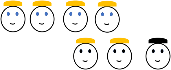
Figure 1. The impossibility of the Conjunction Fallacy

Part of the reason why the conjunction fallacy has been so influential is that, even after the relevant classical probability picture is explained, there is a ‘feeling’ that the statement ‘the individual has blond hair and blue eyes’ seems more correct that the statement ‘the individual has blond hair’. It is this persistence that has often been considered the hallmark of probabilistic paradoxes (Gilboa, Reference Gilboa2000).

In the case of the Scandinavian person, the application of classical probability theory is very direct (because of the set-theoretic nature of the problem). In the original demonstration Tversky and Kahneman (Reference Tversky and Kahneman1983) reported, the constraint may appear superficially less strong. In one of their experiments, a hypothetical person, Linda, was described very much like a feminist and not at all like a bank teller. Participants were asked to rank order according to relative probability a series of statements about Linda, including the statements that she is just a bank teller (considered unlikely given the description) and that she is a bank teller and a feminist (the feminist property by itself would be seen as very likely). Many participants (well over 50%) ranked the conjunction as more likely than the individual premise. One might think that, as in this case there is no obvious sample space, the conjunction constraint may apply more loosely. But this is incorrect. All inferences according to classical probability theory require a sample space and in this case the relevant one consists of all possible Linda’s we can imagine, following the initial description.

Classical probability theory cannot allow e.g. $Prob\left( {F\& BT} \right) > Prob(BT)$, where F = feminist, BT = bank teller in the Linda problem, that is, a conjunction can never be more likely than the marginal. A straightforward application of classical probability theory in the case of the conjunction fallacy would assume that the evaluation participants are making exactly corresponds to a comparison of $Prob\left( {F\& BT} \right)$ with $Prob(BT)$. So, if participants consider the former as more likely than the latter, then they are incorrect. However, what if instead participants mentally compute probabilities in a different way? Notably, suppose that when they compute the conjunction they make one set of assumptions about Linda and when they compute the marginal a different set of assumptions. Call these different sets of assumptions A1 and A2. Then, participants would be comparing $Prob\left( {F\& BT|A1} \right)$ with $Prob(BT|A2)$, and (fairly trivially) observe that the conditionalizations are now on different variables. Under such circumstances, depending on exactly how A1 and A2 affect the corresponding inferences for the conjunction and the marginal, we can have any of $Prob\left( {F\& BT|A1} \right) > Prob(BT|A2)$, $Prob\left( {F\& BT|A1} \right) = Prob(BT|A2)$, $Prob\left( {F\& BT|A1} \right) < Prob(BT|A2)$, and there is no longer a conjunction fallacy! However, decision theorists rarely consider such models, because there are no prior grounds for assuming differences in e.g. assumptions for considering each probability term, as above.

Note that the conjunction fallacy has been extensively replicated. There has been a consideration of a large number of possible confounds, including relating to conversational implicatures (cf. Dulany & Hinton, Reference Dulany and Hilton1991; Grice, Reference Grice, Cole and Morgan1975), possible misunderstanding on the meaning of the conjunction etc. (Moro, Reference Moro2009, provides a review of these issues). The overall conclusion is that, even when all corrective procedures are employed, there is a residual conjunction fallacy.

Even though the conjunction fallacy is a judgment inconsistent with the rules of classical probability theory, this does not preclude that there is an alternative system for probabilistic assignment which might allow probabilities as $Prob\left( {F\& BT} \right) > Prob(BT)$. Our main focus is quantum probability theory, the rules for how to assign probabilities to events from quantum mechanics, without any of the physics. Quantum mechanics is of course a theory of physics, but the pioneering scientists who developed quantum mechanics also had to invent a new theory of probability, as classical probability theory is inconsistent with many of the processes assumed by quantum mechanics. Quantum probability theory has had a fruitful history of application in cognitive science (e.g., Asano, Basieva, Khrennikov, Ohya, & Tanaka, Reference Asano, Basieva, Khrennikov, Ohya and Tanaka2012; Busemeyer & Bruza, Reference Busemeyer and Bruza2011; Haven & Khrennikov, Reference Haven and Khrennikov2013; Khrennikov, Reference Khrennikov2010; Pothos & Busemeyer, Reference Pothos and Busemeyer2013) and additionally there have been some fairly precise proposals for how quantum-like representations can emerge from neuronal interactions (e.g., Khrennikov, Basieva, Pothos, & Yamato, Reference Khrennikov, Basieva, Pothos and Yamato2018).

Quantum probability theory approaches probabilistic assignment in a radically different way, compared to classical probability theory. In classical probability theory, the basis for probabilistic assignment is subsets of sample spaces. In quantum probability theory, instead question outcomes corresponds to subspaces in a multidimensional vector space, and probabilistic assignment concerns the overlap between subspaces and a so-called state vector, which represents the system of interest. Many of these concepts might be unfamiliar to readers, so we proceed with a brief introduction to quantum theory, eschewing most technical detail and technical elaborations (for a more rigorous introduction for psychologists see e.g. Yearsley & Busemeyer, Reference Yearsley and Busemeyer2016).

In quantum theory question outcomes are represented as subspaces in a large vector space (this vector space has some additional properties, which we need not consider here). In most introductory illustrations of quantum theory, such subspaces are one-dimensional (in which case they can be called rays). For example, in Figure 2, we are representing a binary question B with two rays, one corresponding to an affirmative response for B (which we denote as B, slightly abusing notation) and one corresponding to a negative response for B (denoted as ∼B). Subspaces can be of any dimensionality and there is an expectation that more complex concepts would be represented with subspaces of higher dimensionality (Pothos, Busemeyer, & Trueblood, Reference Pothos, Busemeyer and Trueblood2013). Probabilistic inference in quantum theory depends on the state vector, mentioned above, which is a normalised vector. The state vector is a representation of all the information we know about the relevant system, whether this is a physical system (in the original applications of quantum theory in physics) or a psychological system, e.g., the mental state of a participant just before answering some questions relevant to an experiment. In Figure 2, the state vector is represented by the vector labelled S. With subspaces and the state vector, we can compute probabilities as the squared length of the projection of the state vector onto the relevant subspace (this way to associate probabilities to subspaces is a fundamental aspect of quantum theory called Born’s rule). Projection is an operation of taking a vector and ‘laying it down’ onto a relevant subspace. For example, in Figure 2, if we are interested in the probability that a participant with mental state S responds affirmatively to the B question, then we have to measure the square of the projection of S along the B ray.

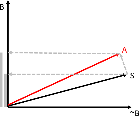
Figure 2. An illustration of how a Conjunction Fallacy can arise with Quantum Probability Theory Inference

Let us introduce some notation. Suppose we are interested in computing probabilities relevant to the Linda version of the conjunction fallacy. Then, envisage two subspaces, one corresponding to the question outcome that she is a BT and one that she is a F. Each subspace is associated with a projector operator, a linear operator which can project the state vector onto the relevant subspace. For the F and BT question outcomes, the projectors can be denoted as ${P_{BT}}$ and ${P_F}$. Then, the projection of the state vector onto e.g. the BT subspace is denoted as ${P_{BT}}|S\rangle$ and the squared length of the projection as $|{P_{BT}}|S\rangle {|^2}$, that is, $Prob\left( {BT} \right) = |{P_{BT}}|S\rangle {|^2}$. Note, we employ here Dirac’s bracket notation, with $|S\rangle$ corresponding to a column vector and $\langle S|$ to the complex conjugate transpose of a $|S\rangle$ (and so a row vector).

The most important distinguishing aspect of quantum probability theory relative to classical probability theory that is presently relevant is that in the former there are two types of questions, compatible and incompatible, while in the latter there are only compatible questions. Incompatible questions are ones for which it is impossible to provide a joint probability distribution. The paradigmatic case of incompatible questions in physics concerns the momentum and position of a microscopic particle. The quantum mechanics implication is that it is impossible to simultaneously know both the position and momentum of such a particle. In psychology, we can think of incompatible questions as ones such that resolving one question creates a different context or perspective for another. The issue of incompatibility in cognition deserves additional remarks that we will further consider shortly.

Let us reiterate the key point that probability is computed through projection (specifically, as the squared length of the projection of the state vector onto the relevant subspace). This should make it clear that certainty, i.e., $Prob\left( {premise} \right) = 1$, corresponds to having the state vector ‘contained’ within the relevant subspace. In Figure 2, for example, if the state vector is aligned with the A subspace, then we would have that $Prob\left( A \right) = 1$. We are thus led to a simple operational approach to what incompatibility is about, namely, it concerns questions such that the relevant subspaces are at oblique angles, so that certainty for one question outcome implies non-zero probability for the outcomes of an alternative question. For example, in Figure 2, we consider two questions, A and B. Question outcome A appears likely given the mental state, represented here as S, since clearly ${P_A}|S\rangle$ would be quite long (this projection is not shown in the figure). By contrast, question outcome B would be less likely, as ${P_B}|S\rangle$ is short. In Figure 2, incompatibility between questions A, B simply means that a state vector aligned with question A has non-zero projections to both B and ∼B and vice versa – it is impossible to find a state vector such that we are simultaneously certain about A or ∼A and B or ∼B; the two questions cannot be simultaneously resolved.

The crucial point is what happens when we want to assess the conjunction A and then B. Because the two questions are assumed to be incompatible, it is not possible to employ the notion of conjunction from classical probability theory (we cannot resolve both A and B simultaneously). Instead, the closest analogue is sequential conjunction, that is, a process of resolving the first conjunct and then the second, $Prob(A\& then\,B)$. This definition is appropriate because it decomposes into the product of a marginal and a conditional, exactly as we would expect from a classical conjunction, that is, $Prob\left( {A\& then\,B} \right) = Prob\left( A \right)Prob(B|A)$. The sequential conjunction corresponds to a sequential projection, in a way analogous to how the probability for a single question outcome corresponds to a single projection. Specifically, $Prob\left( {A\& then\,B} \right) = |{P_B}{P_A}|S\rangle {|^2}$. This operation involves projecting the state vector first onto the A subspace, which is ${P_A}|S\rangle$, and then taking the ${P_A}|S\rangle$ vector and projecting it onto the B subspace, exactly as shown in Figure 2. But, it can be immediately seen in Figure 2 that $|{P_B}{P_A}|S\rangle {|^2} > |{P_B}|S\rangle {|^2}$. We have produced an example in quantum theory which shows $Prob\left( {A\& then\,B} \right) > Prob(B)$.

Let us illustrate how this can be done numerically. Let us introduce angle s, corresponding to the angle between state vector S and question outcome ∼BT and angle t, corresponding to the angle between state vector S and question outcome A. We also note projectors for one-dimensional subspaces can be computed in a simple way as, e.g., ${P_B} = |B\rangle \langle B|$. Recall that $|B\rangle$ is a column vector and in a real space $\langle B|$ would be the corresponding transpose. For example, if $|B\rangle = \left( {\matrix{ a \cr b \cr } } \right)$, then $|B\rangle \langle B| = \left( {\matrix{ a \cr b \cr } } \right)\left( {\matrix{ a & b \cr } } \right) = \left( {\matrix{ {a^2 } & {ab} \cr {ab} & {b^2 } \cr } } \right)$. Note that $\langle B|B\rangle = \left( {\matrix{ a & b \cr } } \right)\left( {\matrix{ a \cr b \cr } } \right) = a^2 + b^2 $, i.e., this is a scalar product. In general, in a real space, for two normalized vectors x, y, the scalar product is $\langle x|y\rangle = \cos \theta$, where $\theta$ is the angle between the two vectors. Accordingly, we have $Prob\left( B \right) = |{P_B}|S\rangle {|^2} = |B\rangle \langle B|S\rangle {|^2} = |\langle B|S\rangle {|^2} = {\cos ^2}(\pi /2 - s) = {\sin ^2}(s)$. Note that in $|B\rangle \langle B|S\rangle {|^2}$ we basically have a vector, $|B\rangle$, and a scalar product, and the length of the former is one – hence, $|B\rangle \langle B|S\rangle {|^2} = |\langle B|S\rangle {|^2}$ Regarding the sequential conjunction, $Prob\left( {A\& then\,B} \right) = \,|{P_B}{P_A}|S\rangle {|^2} = |B\rangle \langle B|A\rangle \langle A|S\rangle {|^2} = |\langle B|A\rangle \langle A|S\rangle {|^2} = {\sin ^2}(s + t){\cos ^2}(t)$. So, if one measures the rate of conjunction fallacy as $Prob\left( {A\& then\,B} \right) - Prob\left( B \right)$, then this simple computation would allow a conjunction fallacy as long as ${\sin ^2}(s + t){\cos ^2}(t) > {\sin ^2}(s)$. There are several combinations of s, t which allow a conjunction fallacy.

There are several points to make. First, this shows how the result $Prob\left( {A\& then\,B} \right) > Prob(B)$ can be correct when using quantum probability theory. So, we have two different perspectives on correctness regarding the conjunction fallacy, from classical probability theory (not allowed under any circumstances, unless of course someone introduces conditionalizing variables, as discussed) and quantum probability theory (can be allowed, depending on the precise arrangement of subspaces and the mental spate). Second, the Figure 2 illustration is extremely restricted. All subspaces are one dimensional subspaces; in general they could have higher dimensionalities. All rays are coplanar, in general they do not have to be. Third, the result $Prob\left( {A\& then\,B} \right) > Prob(B)$ can be produced only if we project to the A subspace first and then the B one; with this approach, we cannot have a conjunction fallacy in a different order. However, we think it is a desirable feature of this approach that not all arrangements of mental states and subspaces can produce a conjunction fallacy. Finally, and most importantly, the fact that quantum probability theory allows the conjunction fallacy as a correct conclusion does not mean that we have an adequate psychological model of what happens in the corresponding empirical situations.

Let us consider first the case of the conjunction fallacies in Tversky and Kahneman (Reference Tversky and Kahneman1983), as exemplified by the Linda problem. The mental state vector can be reasonably said to be close to the ray for feminism (= A in Figure 2) and away from the ray for bank teller (= B in Figure 2). Then, computing the conjunction in the order of feminism first and then bank teller, we have $|{P_{BT}}{P_F}|S\rangle {|^2} > |{P_{BT}}|S\rangle {|^2}$, as required. Busemeyer, Pothos, Franco, and Trueblood (Reference Busemeyer, Pothos, Franco and Trueblood2011); Asano, Basieva, Khrennikov, Ohya, and Yamato (Reference Asano, Basieva, Khrennikov, Ohya and Yamato2013) essentially modelled the conjunction fallacy and related fallacies with a quantum probability model along these lines (but not restricted to one dimensional subspaces or a two dimensional overall vector space). Psychologically, we require the assumptions that the questions of feminism and bank teller are incompatible and that the feminism question is evaluated before the bank teller one. The former assumption appears fairly natural for the Linda problem, for example, perhaps accepting that Linda is a feminist can lead to a perspective or context that makes us re-evaluate the possibility that she is a bank teller. The latter assumption is perhaps benign as well, since there are various psychological views according to which more likely premises benefit from a degree of primacy (e.g., Gigerenzer & Goldstein, Reference Gigerenzer and Goldstein1996).

Let us consider next how quantum probability theory could accommodate the conjunction fallacy in Tentori et al. (Reference Tentori, Bonini and Osherson2004). In this case, the application of quantum theory would have to involve a computation like $|{P_{BE}}{P_{BH}}|S\rangle {|^2} > |{P_{BE}}|S\rangle {|^2}$ (we can reassure ourselves that there would be some arrangement along the lines of Figure 2 that would reproduce the conjunction fallacy, that is, by having rays for the question outcomes BE and BH analogous to the rays for A and B). In this case, however, the intuition from classical probability theory is extremely strong. In other words, understanding the question of whether a Scandinavian person is likely to have blue eyes vs. blonde hair and blue eyes evokes a picture of probabilities as subsets of an overall sample space: there is a subset of Scandinavian individuals with blonde hair, a subset with blue eyes etc. With such a (classical) picture of probabilities it is very difficult to see how the intersection (i.e., conjunction) could ever be more probable than either marginal (cf. Figure 1). The application of quantum theory in this case, requires a rethinking of how questions can be interpreted within a quantum cognitive model.

To address this conundrum we need to recognize the semantics of what it means in quantum probability theory to resolve sequences of incompatible questions. Resolving a question implies a unique perspective for other incompatible questions. Therefore, the same Question A resolved from a baseline perspective vs. the perspective following the resolution of an incompatible Question B should be considered as separate questions. In classical terms, we must separate out the sample spaces. We have one for the baseline perspective of A and a different sample space for each version of A following resolution of each different question incompatible with A. That is, if a series of questions is incompatible, every time we respond to a question, this creates a different perspective for the probabilities relevant to subsequent questions. In more psychological terms, resolving a question creates a unique context for subsequent incompatible questions, so that these subsequent questions have to be understood as different, compared to version answered either in isolation or prior to other incompatible questions.

Given these ideas, if we want to apply quantum probability theory to Tentori et al. (Reference Tentori, Bonini and Osherson2004) example, we have to recast our notion of sample space as in Figure 3. First of all, assume that the questions ‘does a person have blue eyes’ and ‘does a person have blonde hair’ are mentally represented as incompatible (we discuss shortly whether representing the two questions as incompatible can be justified in this case). Following from the ideas in the previous paragraph, resolving one question after the other vs. in isolation should correspond to slightly different versions of the question. Let us consider the question ‘does a person have blue eyes’ and assume that in isolation the meaning of the question is exactly as stated. The sample space in the top of Figure 3 corresponds to asking the question ‘does a person have blue eyes’ in isolation and so we can easily compute that $Prob\left( {blue\,eyes} \right) = 1/3$. If we now ask ‘does a person have blonde hair and (then does a person have) blue eyes’, then incompatibility means that the blue eyes question has to be interpreted somewhat differently, compared to isolation. What would be this different interpretation? Without a more detailed model it is impossible to know. But, for the purposes of illustration, we can make some assumption, for example, let us suppose that the different meaning is ‘blond eye lashes’ (perhaps our participant is confused when seeing the blonde hair question and, by association, instead of understanding the blue eyes question as intended, he confuses it with one about blond eye lashes). In Figure 3, calculation is now based on the sample space in the bottom, so that $Prob\left( {blond\,hair\& then\,blue\,eye{s_{blond\,hair}}} \right) = 4/5$. To reiterate the key point, blue eyes _{blond hair}= ‘blond eye lashes’ Crucially, there is no fallacy any more, since we can have $Prob\left( {blond\,hair\& then\,blue\,eye{s_{blond\,hair}}} \right) > Prob\left( {blue\,eyes} \right)$. The marginal is taken from one sample space and the (sequential) conjunction from a different sample space. Because these probabilities are taken from different sample spaces, they no longer have to be consistent with each other, as required by classical probability theory, and the conjunction can appear as higher than the marginal (for a more detailed exposition of these ideas see Pothos, Busemeyer, Shiffrin, & Yearsley, Reference Pothos, Busemeyer, Shiffrin and Yearsley2017).

Figure 3. How having different sample spaces can allow the Conjunction Fallacy

Would participants be justified in employing two different versions of the blue eyes question in Tentori et al.’s (Reference Tentori, Bonini and Osherson2004) experiment? No and so we have to conclude that the result of Tentori et al. (Reference Tentori, Bonini and Osherson2004) does indeed reflect a fallacy, though possibly one of misrepresenting as incompatible questions which are in reality compatible. What about the Linda example (and its variants) in Tversky and Kahneman (Reference Tversky and Kahneman1983)? In this case there are more grounds to expect that participants may interpret the question about whether Linda is a bank teller or not differently, depending on whether there is a prior question about feminism or not. In isolation, the question perhaps is interpreted as one corresponding to whether Linda is employed as a bank teller. After the feminism question, the bank teller one is perhaps interpreted as a question of whether being a bank teller is a typical profession for feminists (perhaps it is not the most likely profession for feminists, in the 80s, but it would not be entirely unlikely either). Either way, the point is that in order to reconcile correctness in probabilistic inference with quantum probability theory, we have to acknowledge that responding to sequences of incompatible questions generates different versions of the questions.

The issue of correctness is somewhat separate from the issue of rationality. Quantum probability theory is a formal framework for probabilistic inference and responding in a way that is consistent with the constraints from quantum probability theory is equivalent to a statement that responding is according to a coherent set of principles. But this falls short of a justification for the rational status of quantum probability theory. However, Pothos et al. (Reference Pothos, Busemeyer, Shiffrin and Yearsley2017) argued that the requirements for the Dutch Book Theorem are fulfilled for quantum probability theory too. So, one of the major formal justifications for the rational status of classical probability theory applies to quantum probability too.

A final issue to address concerns the relevance of quantum probability theory to cognition. It seems there is no doubt that, in some cases at least, human decision makers employ incompatible representations, as is indicated by the several reports of behavior inconsistent with classical probability theory, but for which simple quantum cognitive models are possible (e.g., see the overviews in Bruza, Wang, & Busemeyer, Reference Bruza, Wang and Busemeyer2015, Pothos & Busemeyer, Reference Pothos and Busemeyer2013, or Wang, Busemeyer, Atmanspacher, & Pothos, Reference Wang, Busemeyer, Atmanspacher and Pothos2013). So, regardless of whether employing incompatible representations is justified or not, it appears that this occurs. But would there be situations when it is justified too? We think this would be the case, for example, when questions can have different meanings depending on context (which could be generated by other questions). That is, in the macroscopic world that concerns most of the decisions we are likely to have to make, incompatibility reflects some kind of contextuality, where the presence of questions can alter the meaning of other ones (note we are employing here the term contextuality in a fairly lay way, to imply dependence on context; in quantum theory there is a more specific sense of contextuality which is presently less relevant, e.g., Cervantes & Dzhafarov, Reference Cervantes and Dzhafarov2018; Dzhafarov, Kujala, Cervantes, Zhang, & Jones, Reference Dzhafarov, Kujala, Cervantes, Zhang and Jones2016). Additionally, there will be situations when a decision alters the state that is relevant for responding to subsequent questions and, in such cases (where there is a possibility of so-called ‘disturbing measurements’) there will be potential for formal understanding employing the notion of incompatibility (Pothos et al., Reference Pothos, Busemeyer, Shiffrin and Yearsley2017; White, Pothos, & Busemeyer, Reference White, Pothos and Busemeyer2014).

Concluding comments

We have seen three frameworks for understanding correctness and rationality, classical logic, classical probability theory, and quantum probability theory. The relevance of classical logic could be discounted fairly easily, e.g., employing arguments concerning the general applicability of deductive rules in everyday decision making (cf. Chater & Oaksford, Reference Chater and Oaksford1993). Note, there is an additional layer of subtlety here, in that the algebraic foundations of classical probability theory actually embody classical logic, but we will ignore this issue here.

Classical probability theory and quantum probability theory provide two strikingly different intuitions for probabilistic inference (and in fact challenge some convergence results in classical probability theory, e.g., Khrennikov & Basieva, Reference Khrennikov and Basieva2014). Note that some of this dependence of context that is one hallmark of quantum incompatibility could be accommodated with classical probability theory too, e.g., through appropriate conditionalizations. But, while such conditionalizations are post hoc, we think it is unlikely that they be convincing to the scientific community. One origin of the radically different pictures for probabilistic inference embodied in these two theories is the reliance of one on sample spaces and set-theoretic operations and the other on vector spaces and the geometry of subspaces/ projections.

Classical and quantum probability theories hardly exhaust the possibilities for formal systems for probabilistic inference. It is possible to specify a hierarchy of probabilistic frameworks, organized in terms of the complexity of the probability rules which are employed (here, complexity has a specific meaning in terms of additional terms which arise in the law of total probability, Sorkin, Reference Sorkin1994). In such a hierarchy the very first element is classical probability theory and the next element quantum probability theory. Thus, it is entirely possible that future work will motivate alternative probability theories in psychology applications, which would themselves lead to alternative notions of correctness (perhaps invoking more elaborate versions of the idea that previous questions can affect the meaning of subsequent ones). Even though it seems unlikely that more elaborate probability theories will be relevant in the modelling of behavior specifically, there may be applications in e.g. artificial intelligence. Either way, the development of decision theory in psychology has brought into sharp focus the idea that correctness in decision making is far from a singular notion and one has to consider carefully how different approaches compare and can be justified.