2. ERROR SOURCES OF GNSS ONE-WAY TIMING

The GNSS timing user obtains the satellite-to-user pseudo-range observation $P_{r, i}^{s} $ in Equation (1) by receiving GNSS signal while decoding the navigation message parameters (Sha et al., Reference Sha, Zhan and Wang2013; Zhang et al., Reference Zhang, Yang, Shao and Yao2019). The satellite position at the time of transmission is calculated according to the ephemeris parameters in the navigation message and then the geometric distance $R_{r}^{s} $ between the satellite and user is determined at the time. The deviation dT ^s(t ^s) between the satellite clock and the system time is calculated according to the parameters of the satellite clock model. The tropospheric refraction delay $T_{r}^{s} $ is calculated according to the empirical Saastamoinen model. The additional delay of the ionosphere $I_{r, i}^{s} $ is corrected by single-frequency ionospheric model or a dual-frequency combination of observations. The internal hardware delay of receiving terminal D _r is calibrated in advance.

(1)$$P_{r,i}^s =R_r^s +c(dt_r (t_r )-dT^s(t^s))+I_{r,i}^s +T_r^s +D_r+\varepsilon _P$$

For the pseudo-range observation in Equation (1), the above delay corrections are deducted to obtain the user receiver clock difference in Equation (2), that is, the deviation between the local time of the user and the system time of GNSS.

(2)$$dt_r (t_r)=\frac{1}{c}(P_{r,i}^s -R_r^s +dT^s(t^s)-I_r^s -T_r^s -D_r)$$

Thus, the difference between local time and GNSS time is obtained. If a user wants to know the bias between their local time and UTC, the traceability model parameters will be applied to calculate the time difference $\Delta t_{\rm{UTC}}$ and correct the user's clock difference as

(3)$$t_{r,{\rm UTC}} =dt_r (t_r )-\Delta t_{\rm{UTC}}.$$

In the above process of realising timing, the main error sources, as shown in Figure 1, affecting one-way timing results are: satellite clock error, ephemeris error, ionospheric additional delay correction error, tropospheric refraction delay correction error, receiving terminal internal delay calibration error and traceability error, among others (Levine, Reference Levine2008). The satellite clock error and the ephemeris error depend on the signal in space (SIS) user range error (URE) of GNSS. According to the BeiDou Public Signal Service Specification, the URE does not exceed 2·5 m (95%). The ionospheric additional delay correction error depends on the correction method applied and the tropospheric refraction delay correction error is relatively small. With the absolute delay calibration method, the internal delay calibration error can generally be controlled within 2 ns (Zhu, Reference Zhu2015). The satellite clock error is completely related to satellites; the ephemeris error and the ionospheric delay residual error are spatially correlated. These three errors can be eliminated or reduced by differential.

Figure 1. Distribution of error sources in GNSS one-way timing.

The traceability error depends on the accuracy of the traceability model parameters broadcast in navigation messages. The International Telecommunication Union (ITU) requires that the system time of a satellite navigation system should trace to UTC and the deviation against UTC should stay within 100 ns (Wang, Reference Wang2014). Thus, the system time of GNSS is directly traced to UTC(k) which is the physical realisation of UTC by timing laboratory k via TWSTFT or GNSS common view time transfer links (Dong and Wu, Reference Dong and Wu2012; European GNSS (Galileo) 2010; Lewandowski and Arias, Reference Lewandowski and Arias2011; Nicolini and Caporali, Reference Nicolini and Caporali2018). Although the traceability deviation is precisely monitored, the error sources from satellites to users in one-way timing cannot be effectively eliminated or reduced due to different paths. The error fluctuates in the range of −40 ns to 30 ns with an average error of about 41 ns (Zhu, Reference Zhu2015).

3. DIFFERENTIAL TIMING METHOD BASED ON TRACEABILITY MODEL PARAMETER

Inspired by the above analysis of one-way timing error sources and the current monitoring method of traceability deviation, a differential timing method by changing the generation of traceability model parameter is proposed. The principle of this method is shown in Figure 2. In the timing master station (TMS), one timing monitoring receiver, referenced to the UTC(k) time and the frequency signal kept by the timing laboratory k, is used to collect the pseudo-range observations by receiving GNSS SIS. The pseudo-range observations of satellites in view are corrected with each error delay correction of one-way timing to obtain the clock difference $dt_{m, i} ( t_{m, i} ) $ of the monitoring receiver at TMS for each satellite with m indicating the TMS. The clock difference represents the time deviation between the system time obtained through satellite i and UTC(k). Then the traceability deviation model parameters are obtained by modelling the traceability deviation $dt_{m, i} ( t_{m, i} ) $ of each satellite at the master control station, and then inserted into the navigation message and sent to the corresponding satellites by the uplink station.

Figure 2. Principle of the proposed differential timing method.

The user timing receiver receives GNSS satellite signals and deducts all the delays from pseudo-range observations to obtain the receiver clock difference $dt_{r, j} ( t_{r, j} ) $ related to each satellite in view. Then the traceability model parameters of corresponding satellites monitored by TMS are further applied to correct the receiver clock error, and the time difference between the user local time and the reference time UTC(k) of TMS is obtained.

(4)$$\Delta t_{r,m,i} =dt_{r,j} (t_{r,j} )-dt_{m,i} (t_{m,i} ),\quad i=j$$

Equation (4) indicates that the proposed method is equal to implementing a timing differential between user and TMS via satellite i. Compared with the traditional GNSS one-way timing method, the advantage of the proposed method is reflected in the change of the manner of generation of traceability deviation that reduces the error sources of the traditional radio navigation satellite system (RNSS) one-way timing and realises timing at nanosecond level. The satellite traceability deviation monitored by the proposed method includes the delay correction error $\varepsilon _{m} $ of TMS, namely satellite clock error, ephemeris error, ionospheric delay correction error, tropospheric delay correction error and monitoring receiver internal delay calibration error. If $\varepsilon _{r} $ represents the traditional RNSS one-way timing error, then the timing error of the proposed method is $\varepsilon _{rm} =\varepsilon _{r} -\varepsilon _{m} $. Considering the satellite clock errors for the same satellite at the user station and the TMS are completely correlated, and the ephemeris error and ionospheric error are correlated with the space, $\varepsilon _{rm} $ is generally smaller than $\varepsilon _{r} $ after differential, especially when the user is close to the TMS. Consequently, the accuracy of the traceability differential timing method is better than that of the traditional one-way timing method. The internal delay calibration error of the receiving terminal is one of the main error sources that affect the timing result of RNSS one-way timing method. To obtain accurate timing results, it is necessary to calibrate accurately the internal delay of the receiver terminal. As far as traceability of the differential method is concerned, the timing result is affected by the relative internal delay between user terminal and the timing monitoring receiver (Romisch et al., Reference Romisch, Zhang and Parker2012). Therefore, users need to determine the relative delay of their terminals against the timing monitoring receiver at TMS which avoids the complicated calibration of receiver internal delay (Young et al., Reference Young, Munson and Meehan2009). Another benefit is that the accuracy of relative delay calibration is more precise and the implementation is simpler and easier (De Bakker et al., Reference De Bakker, Tiberius and van der Marel2012; Zhu, Reference Zhu2015).

4. ANALYSES OF REALISING THE PROPOSED METHOD ON BEIDOU GEO SATELLITES

BeiDou GEO satellites can always be seen by the China area and therefore can be utilised at a high rate. The BeiDou master control station can update navigation message information in real time (Schempp et al., Reference Schempp, Burke and Rubin2008; Xiao et al., Reference Xiao, Sun and Li2016). Five sites surrounding the China area are selected as the test sites: Changchun in the northern region, Sanya and Kunming in the southern, Kashi in the western, and Shanghai in the eastern. The BDT is steered to UTC(NTSC), kept by the National Time Service Center (NTSC) which is located at Xi'an, China. Thus, this timing laboratory is taken as the TMS. All the five sites as well as Xi'an can observe the three GEO satellites (80^° E, 110·5^° E, 140^° E) of BDS-3 for 24 h a day with elevation of not less than 10^°. The time period of observing BeiDou MEO satellites in the same condition is only about 6 h. That is to say, in order to achieve uninterrupted timing throughout one day for single-satellite one-way timing, users need to track at least four MEO satellites in turn, while only one GEO satellite is sufficient.

In addition, compared with MEO satellites, the traceability differential method based on GEO satellites is less affected by ephemeris and ionospheric delay errors. The residual ephemeris error can be expressed as:

(5)$$\Delta \tau _{AB} \le \frac{1}{c}\cdot \frac{\left| {{\mathop{d} \limits^{\rightharpoonup}}_{AB} } \right|}{r}\cdot \left| {{\mathop{\varepsilon} \limits^{\rightharpoonup}}_S } \right|,$$

where ${{\mathop{d} \limits^{\rightharpoonup}}_{AB}}$ is the distance between user and TMS, ${{\mathop{\varepsilon} \limits^{\rightharpoonup}}_S }$ is the satellite position error, r is the distance from satellite to TMS.

From Equation (5), one can see that the residual ephemeris error is inversely proportional to the distance from satellite to TMS. This means that, for certain ${{\mathop{\varepsilon} \limits^{\rightharpoonup}}_S }$ and ${{\mathop{d} \limits^{\rightharpoonup}}_{AB}}$, the higher the satellites' orbits, the smaller the residual ephemeris errors. BeiDou GEO satellites orbit at the altitude of 35,786 km which is 1·66 times higher than that of BeiDou MEO satellites. When the distance between user and TMS is 1,000 km and the satellite position error is 10 m, the residual ephemeris error based on the MEO satellites is 0·46 m, about 1·5 ns, while the residual ephemeris error based on the GEO satellites is only 0·28 m, about 0· 9ns.

Because GEO satellites are almost stationary, the variation of ionospheric pierce point (IPP) of GEO satellites for fixed locations in the China region is very small. The latitude and longitude variation of IPP for the China area is no more than 2^°. The differential ionospheric error corresponding to the B1 frequency of the BeiDou navigation signal can be expressed as:

(6)$$\begin{aligned} \Delta I_{rm} & =\vert {I_r -I_m } \vert =\frac{40\cdot 3}{f^2}\cdot \left| {\frac{1}{\sin \phi_r^{IPP} }\cdot {\rm VTEC}_r -\frac{1}{\sin \phi_m^{IPP} }\cdot {\rm VTEC}_m } \right| \\ & \approx \frac{40\cdot 3}{f^2}\cdot \overline {{\rm VTEC}} \cdot \left| {\frac{1}{\sin \phi_r^{IPP} }-\frac{1}{\sin \phi_m^{IPP} }} \right| \\ & \approx {\rm 1}\cdot {\rm 62}\cdot \left| {\frac{1}{\sin \phi_r^{IPP} }-\frac{1}{\sin \phi_m^{IPP} }} \right| \\ \end{aligned}$$

where I _m denotes the ionospheric delay of Xi'an station, I _r is the ionospheric delay of the five sites, $\phi _{m}^{{\rm IPP}} $ is the elevation of IPP for Xi'an reference station, $\phi _{r}^{{\rm IPP}} $ is the elevation of user IPP, andVTEC_r, VTEC_m are the vertical total electronic content corresponding to IPP of user and TMS. $\overline {{\rm VTEC}} $ is the average total vertical electronic content over TMS and the user.

Table 1 provides the elevation of IPP, $\phi _{i}^{{\rm IPP}} $, when five BeiDou GEO satellites are observed at Xi'an and the other five stations, respectively. The corresponding differential ionospheric delay residuals between the five stations and Xi'an, Δ I _rm, are also listed. It can be seen that even if the difference between IPP elevations of Kashi and Xi'an reaches 20^° when simultaneously observing SV01, the differential ionospheric delay residual is only 1·9 m. The result is 1·35 m when Changchun and Xi'an observe SV05 at the same time. Except for the above two cases, the residual ionospheric delays for all the other cases are within 1 m. It is worth noting that the ionospheric delay residuals in the above table only account for the difference in ionospheric delay caused by the difference of elevation. As a matter of fact, the total vertical electron content over different stations is different and changes in complicated ways with time and space. Therefore, the differential ionospheric delay residuals may be larger than those in Table 1.

Table 1. Differential ionospheric delay residual respectively between five sites and Xi'an via different satellites (Unit: meter).

5. EXPERIMENT VERIFICATION AND ANALYSIS

5.1. Setup of experiment platform

In order to test the feasibility of the proposed method, an experiment verification platform is built based on the UTC(NTSC) time frequency signal kept by the timing laboratory of NTSC, as shown in Figure 3.

Figure 3. Experiment verification platform of BeiDou traceability differential timing method.

The monitoring equipment in TMS mainly includes a timing receiver, a time interval counter (TIC), an industrial personal computer (IPC) and data processing software. TMS locates at NTSC and takes UTC (NTSC) as the reference time and frequency signal. The receiver receives BeiDou SIS, completes the pseudo-ranges measurement, decodes the navigation message and simultaneously outputs the 1PPS timing signal. The TIC measures the time difference between the receiver's output 1PPS signal and the UTC(NTSC) 1PPS reference signal. The IPC collects the receiver observations and the time difference measured by TIC. The software running on the IPC first calculates the receiver clock bias corresponding to each satellite in view of TMS. Then, according to the measured time difference of TIC, the time difference between BDT derived by each visible satellite and UTC(NTSC), i.e., the satellite traceability deviation, is obtained. A time period of some satellite traceability deviations is modelled. Finally, the traceability deviation model parameters of this satellite are obtained. The model parameters are related with satellites with fixed update period.

The experiment sites were equipped with atomic clocks. The time signal output by the atomic clock was used as the reference signal of the experiment device and the local time of the experiment sites. The monitoring equipment at the experiment site works in the same way as that of TMS. The receiver clock difference at the experiment site is obtained via the same process as that of TMS. Then, the traceability deviation model parameters monitored by TMS are received and applied by extrapolating the model parameters. The predicted traceability deviation is further used to correct the receiver clock difference of the experiment site. As a result, the time difference between the local time of experiment site and UTC (NTSC) is obtained.

The TMS was selected at Xi'an, and the experiment sites were selected respectively at Lin'tong, Sanya and Kashi. TWSTFT links of Xi'an–Sanya and Xi'an–Kashi (Huang et al., Reference Huang, Yang and Cheng2019) and an optical fibre time transfer link of Lintong–Xi'an (Meng et al., Reference Meng, Liu and Wang2018) are operated simultaneously as the verification reference for evaluating the performance of the traceability differential timing method. The accuracy of time transfer of the TWSTFT link is better than 2 ns and the optical fibre link performs even better.

5.2. Experiment process and evaluation method

Before the experiment is carried out, the system delay of the platform is calibrated in advance. First, the system delay difference between the TWSTFT equipment and the equipment of this platform is determined to ensure that the measurement start–stop points are consistent. The second step is to determine the differential delay of equipment at TMS and the experiment site. The near-zero baseline comparison method with common reference clock is used to determine the differential delay between the experiment device and TMS equipment. The difference is taken as the systematic difference and deducted from the experiment result. The average value of the delay difference is 1·6 ns according to the measured delay difference of 10 days in Figure 4.

Figure 4. Delay difference between experimental equipment and TMS.

The effect of the traceability differential timing method is analysed in terms of timing and positioning at each test site. For timing, the performance of the proposed method is compared with that of the RNSS one-way timing. The root mean square error ${\rm RMS}_{\rm{time}}^{uc} $ of the difference between traditional timing results and the reference Ref are calculated. Meanwhile, the root mean square error ${\rm RMS}_{\rm{time}}^{c} $ of the difference between traceability differential timing results and the reference Ref are also computed to measure the timing performance of the proposed method.

(7)$$\begin{align} {\rm RMS}_{\rm{time}}^{uc} &=\sqrt {\frac{1}{N}\sum\limits_{i=1}^N {({\rm Res}_{uc,i} -{\rm Ref}_i )^2} }\label{eq7} \end{align}$$

(8)$$\begin{align} {\rm RMS}_{\rm{time}}^c &=\sqrt {\frac{1}{N}\sum\limits_{i=1}^N {({\rm Res}_{c,i} -{\rm Ref}_i )^2} }\label{eq8} \end{align}$$

The positioning results with and without employing the traceability model parameters are respectively compared with the reference position determined by survey. The index of root mean square error is used as the analysis criterion as well. As shown in Equations (9) and (10), $( x_{0} , \; y_{0} , \; z_{0} ) $ is the surveyed position of the experiment site and $( x_{i}^{uc} , \; y_{i}^{uc} , \; z_{i}^{uc} ) $ represents the standard single point positioning (SPP) results by which pseudo-ranges are corrected with the traceability differential timing parameters and $( x_{i}^{c} , \; y_{i}^{c} , \; z_{i}^{c} ) $ are the standard SPP results without the correction.

(9)$$\begin{align} {\rm RMS}_{3D}^{uc} &=\sqrt {\frac{(x_i^{uc} -x_0 )^2+(y_i^{uc} -y_0)^2+(z_i^{uc} -z_0 )^2}{N}}\label{eq9} \end{align}$$

(10)$$\begin{align} {\rm RMS}_{3D}^c &=\sqrt {\frac{(x_i^c -x_0 )^2+(y_i^c -y_0 )^2+(z_i^c -z_0)^2}{N}}\label{eq10} \end{align}$$

In addition, the timing improvement ratio of the proposed method against the RNSS one-way timing results is provided in Equation (10). The improvement ratio of positioning is defined as the position errors with traceability differential deviation correction against that of the standard SPP by Equation (12).

(11)$$\begin{align} {\rm Tim}\_{\rm ratio}&=\frac{{\rm RMS}_{\rm{time}}^{uc} -{\rm RMS}_{\rm{time}}^c }{{\rm RMS}_{\rm{time}}^{uc} }\times 100\%\label{eq11} \end{align}$$

(12)$$\begin{align} {\rm Pos}\_{\rm ratio}&=\frac{{\rm RMS}_{3D}^{uc} -{\rm RMS}_{3D}^c }{{\rm RMS}_{3D}^{uc} }\times 100\%\label{eq12} \end{align}$$

5.3. Analysis of timing results

Figure 5 shows the results of RNSS one-way timing and traceability differential timing for Lintong from 22 September to 2 October 2015. Figure 6 shows the results for Kashi from 20 to 23 October 2015. Figure 7 shows the results for Sanya from 10 to 20 May 2016. The comparison of BeiDou traceability differential timing results with those of RNSS one-way timing is shown in Table 2.

Figure 5. RNSS one-way and traceability differential timing results at Lintong.

Figure 6. RNSS one-way and traceability differential timing results at Kashi.

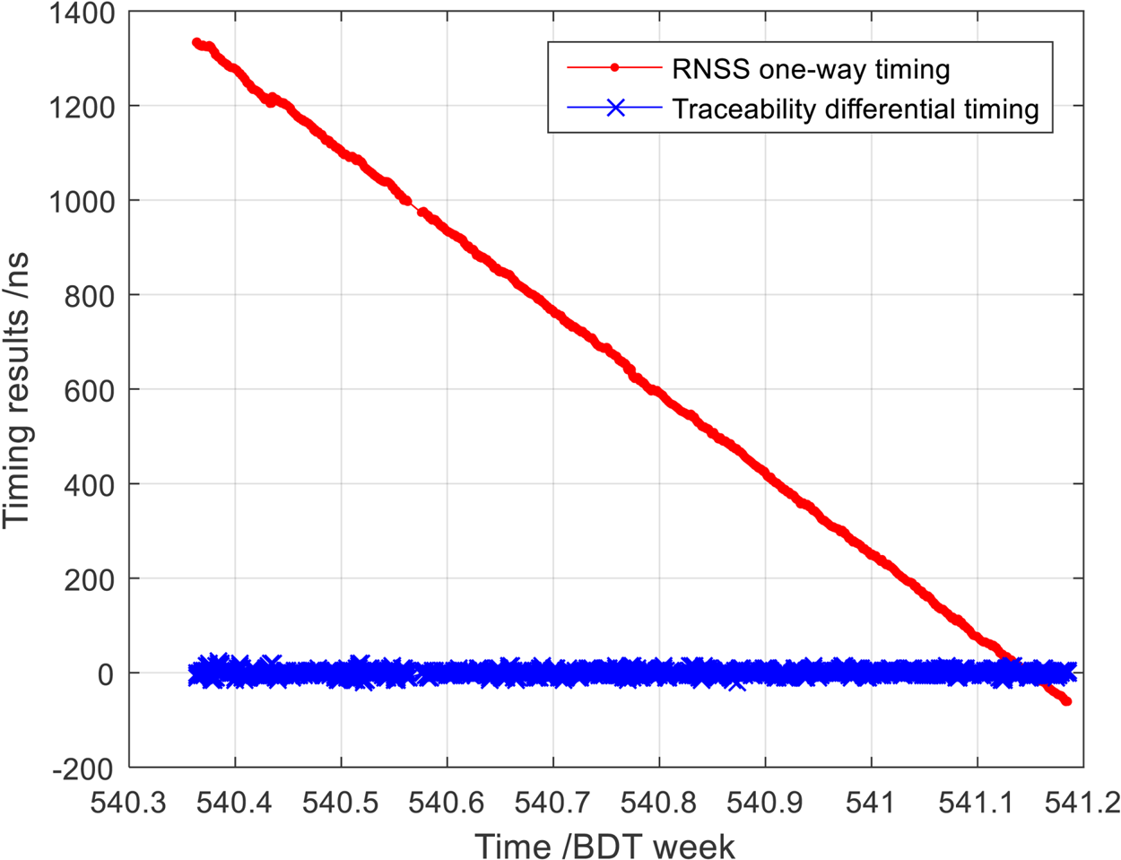
Figure 7. RNSS one-way and traceability differential timing results at Sanya.

Table 2. Comparison of BeiDou traceability differential timing results with RNSS one-way timing results (Unit: ns).

According to the results of the Lintong, Sanya and Kashi experiment sites, shown in Figures 5–7 and Table 2, it can be concluded that a timing accuracy of better than 10 ns can be achieved with the traceability differential model parameters generated by the proposed method. Compared with the traditional RNSS one-way timing method, the improvement ratio of this new timing method is at least 60%.

It should be specially stated that during the experiment at Sanya the GEO satellites were maneuvered and the ephemeris had large errors which led to a very large drift in the one-way timing results. However, the results of the traceability differential timing were still accurate. This indicates the restraining effect of ephemeris error of the traceability differential timing method.

5.4. Analysis of position results

In implementing standard SPP, different satellite clock time must be corrected to the common system time of the satellite navigation system. If pseudo-ranges are further corrected with the traceability differential deviation, the SPP results can be improved. The principle is similar to that of local differential position with only one reference station. This is because the traceability differential deviation includes ephemeris error, satellite clock error and ionospheric error which are correlated with those of the user. If the traceability differential deviation is applied to correct the pseudo-ranges of the user before implementing SPP, then the errors will be weakened and thereby the accuracy of user positioning will be improved.

In order to verify the improvement effect of this method on positioning, experiments were carried out in Lintong, Kashi and Sanya. The SPP results with and without the correction of traceability differential deviation are respectively shown in Figures 8–10. Table 3 shows the three-dimensional position error at Lintong, Kashi and Sanya with and without application of traceability differential deviation. It can be seen from the data in the table that the position error is reduced from 5·13 m to 1·56 m for Lintong, from 19·36 m to 10·03 m for Kashi and from 5·80 m to 3·99 m for Sanya, respectively. The difference in positioning improvement effect for the three experiment sites with this method is because it depends on factors such as the distance between the experiment site and TMS and the latitude of the experiment site (Feng et al., Reference Feng, Chen and Wu2011).

Figure 8. Positioning errors of standard SPP and traceability differential SPP at Lintong

Figure 9. Positioning errors of standard SPP and traceability differential SPP at Kashi.

Figure 10. Positioning errors of standard SPP and traceability differential SPP at Sanya.

Table 3. Comparison of positioning errors for traceability differential SPP and standard SPP (Unit:meter).