


1. Introduction
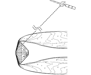
Mars entry flight conditions involve velocities up to  $5\text {--}8\ \textrm {km} \ \textrm {s}^{-1}$, resulting in aerodynamic heating that rapidly dissociates the free stream atmosphere in the shock layer. The production of electrons and ions creates a region of ionized flow or plasma around the vehicle that may cause communication blackout. Radio signals from the spacecraft, typically directed at a relay orbiter near Mars, can be degraded (brownout) or completely attenuated (blackout) by the plasma sheet, as shown in figure 1. The amount of free electrons plays an important role as the natural resonant plasma frequency has a square root dependence on the electron number density. When the plasma frequency approaches or exceeds the radio frequency, signal degradation is likely (Morabito et al. Reference Morabito, Kornfeld, Bruvold, Craig and Edquist2009). As the compressed gas from the shock layer flows to the wake region behind the vehicle where the ionization levels are lower, the plasma flow is rapidly cooled and rarefied by expansion allowing for the propagation of electromagnetic waves (Takahashi, Nakasato & Oshima Reference Takahashi, Nakasato and Oshima2016). Consequently, Mars entry vehicles such as the Mars science laboratory, Mars Pathfinder and ExoMars Schiaparelli had an antenna located on their backshell.

Figure 1. Radio frequency blackout for flow over reentry capsule.
Generally, blackout analysis depends on predictions of the electron number densities and collision frequencies around the reentry vehicle obtained from thermochemical non-equilibrium hypersonic computational fluid dynamics (CFD) simulations. Both of these parameters depend on the density-velocity conditions along the trajectory and are influenced by gas chemistry as well as the distribution between energy modes, i.e. the translational, rotational, vibrational and electronic temperatures of gas species. Electron production is low in the beginning of the reentry due to the low neutral density of the atmosphere. It then increases to a maximum approximately at the time of the peak aerodynamic heating. Afterwards, electron production diminishes due to the now low-speed capsule. Subsequently, to model the electromagnetic wave propagation through the plasma, one can use various methods including the plasma frequency approach (Morabito Reference Morabito2002; Morabito et al. Reference Morabito, Schratz, Bruvold, Ilott, Edquist and Cianciolo2014; Ramjatan et al. Reference Ramjatan, Magin, Scholz, Van der Haegen and Thoemel2016), geometrical optics or ray tracing (Delfino Reference Delfino2004; Vecchi et al. Reference Vecchi, Sabbadini, Maggiora and Siciliano2004), or using a finite differencing scheme to solve the Maxwell equations directly (Takahashi et al. Reference Takahashi, Nakasato and Oshima2016). The plasma frequency method is the simplest while other complex methods involve direct simulation of the radio wave as it traverses the plasma. Only these more elaborate methods are able to accurately model the wave phenomena of reflection, refraction (ray bending), phase modulation and spectral broadening of the radio signal. In this paper ray tracing is demonstrated as a novel method for Mars blackout analysis by studying the ExoMars Schiaparelli blackout period of which no predictions have been made in the literature so far. Simultaneously, a novel approach that economizes on computational resources by decoupling the calculation of electron density from the CFD simulations is introduced. Typically, CFD simulations for blackout analysis incorporate expensive non-equilibrium thermochemistry models including separate conservation equations for each of the species and for the different temperatures (or energy modes) that are considered.
1.1. State-of-the-art in blackout analysis
Regarding Mars blackout predictions, varying levels of modelling complexity have been used. The accuracy of blackout or brownout predictions depends on the electromagnetic (EM) wave propagation method and the uncertainty of the electron prediction from CFD simulations.
For the Mars Pathfinder mission, Morabito examined the 30 s blackout of the X-Band radio signal of the Mars Pathfinder mission using the plasma frequency approach (Morabito Reference Morabito2002). This method compares the maximum electron density along the line of sight (LOS) from the transmitter on the spacecraft to the receiving satellite with a critical electron density. This critical electron density occurs when the plasma frequency is equal to the radio frequency resulting in signal degradation. Morabito used the JPL Horton program (Horton Reference Horton1964), a one-dimensional (1-D) semi-analytical flow solver assuming chemical and thermal equilibrium, to calculate the electron density at the stagnation point. Equations of continuity, momentum and energy were integrated with respect to the flow direction x and applied across a normal shock where the effects of diffusion and radiative transfer were considered negligible. Using a frozen flow assumption, the electron density in the wake was estimated by assuming that the electron density in the stagnation region remains constant as the gas flows around the spacecraft into the wake. Morabito compared these results with the Langley aero-thermodynamic upwind relaxation algorithm (LAURA) assuming thermal and chemical non-equilibrium and extracted electron densities along the LOS. There was reasonable agreement in the electron density prediction between Horton and LAURA. He compared the electron density from CFD simulations to the critical density of the spacecraft's frequency band and found that the electron density in the wake region exceeded the critical X-band electron density during the first 20 s of the 30 s blackout period (Morabito Reference Morabito2002). He explained that the continuation of the blackout period during the last 10 s was likely due to high Doppler dynamics and any attenuation, reflection or spectral broadening effects, which could have lowered the signal to noise (SNR) ratio. The latter explanation of a low SNR was observed when the radio signal was regained after the blackout period.
The Phoenix spacecraft with a UHF frequency band did not suffer a signal outage (blackout) but experienced varying levels of reduced signal strength (brownout) during its entry (Morabito et al. Reference Morabito, Kornfeld, Bruvold, Craig and Edquist2009). In this study, Morabito et al. conducted a more detailed communication analysis where the predicted attenuation was calculated by numerically integrating a radio wave absorption equation along the LOS using the electron density distribution from LAURA. The effect of collisions on the attenuation was neglected. The LOS method neglects refraction, which may bend radio waves around plasma regions with large amounts of electrons. The estimation of the attenuation along the propagation path to the relay orbiters were consistent with the observed values within the expected factor of 10 uncertainty of the LAURA electron number density estimates in the wake region. Morabito et al. describes that the observed signal fades provide evidence that reflection and absorption of signal energy off of the plasma around Phoenix was responsible for the brownout (Morabito et al. Reference Morabito, Kornfeld, Bruvold, Craig and Edquist2009). Similarly, Morabito et al. examined the 70 s UHF blackout and brownout of the Mars science laboratory (MSL) using the plasma frequency method. LAURA was also used to retrieve the electron density field along the LOS and the measured SNR degradation periods lined up well with the predicted electron density curves (Morabito et al. Reference Morabito, Schratz, Bruvold, Ilott, Edquist and Cianciolo2014). Thus, reviewing previous blackout studies for Mars entries, retrieving the electron density from non-equilibrium CFD simulations and using the plasma frequency method along the LOS was a common approach. This work applies ray tracing to examine the reflection and refraction of radio waves in the wake flow of the ExoMars Schiaparelli vehicle.
1.2. Novelty of current work
Examining radio blackout using CFD can be computationally expensive due to advanced thermochemical modelling that require the simulation of numerous ionized species and internal temperatures. The computational stiffness and simulation time further increases as one has to account for associative ionization, charge exchange and electron-impact ionization reactions in the chemical mechanism. In addition, accounting for multi-temperature models further increases the dimension of the system to be solved. Regarding Earth reentry missions, Ramjatan et al. performed CFD simulations of small cone-shaped reentry vehicles involving different cone angles, altitudes and velocities to examine the feasibility of communicating during the blackout phase (Ramjatan et al. Reference Ramjatan, Magin, Scholz, Van der Haegen and Thoemel2016). Simulations were done in chemical non-equilibrium with 11 chemical species with 26 chemical reactions. For Martian reentry missions, the blackout work of Morabito et al. involved running three-dimensional (3-D) CFD computations at 10 instances of the MSL spacecraft (Morabito et al. Reference Morabito, Schratz, Bruvold, Ilott, Edquist and Cianciolo2014). Morabito et al. performed simulations at chemical and thermal non-equilibrium (a two-temperature model) with 20 species for the Martian atmosphere. Likewise, Morabito et al. performed similar analysis for the Mars Pathfinder mission employing a two-temperature model with 18 species (Morabito Reference Morabito2002). This required solving 18 species continuity equations, 3 momentum equations and 2 energy equations resulting in 23 simultaneously solved equations at each computational point (Morabito Reference Morabito2002). Similarly, Takahashi et al. examined the blackout of the European Space Agency's atmospheric reentry demonstrator (ARD) by performing 3-D CFD simulations in thermal chemical non-equilibrium with 11 chemical species with 49 reactions in air (Takahashi et al. Reference Takahashi, Nakasato and Oshima2016). Thus, introducing multi-temperature models with extensive reaction mechanisms can quickly increase the computational cost in retrieving the electron density.
The first novelty of this work is to apply a computationally inexpensive Lagrangian approach titled LARSEN (Boccelli et al. Reference Boccelli, Bariselli, Dias and Magin2019), to compute the electron density field from a baseline CFD solution that was solved with only six neutral species. A more elaborate thermochemical model consisting of 14 species is applied to recompute the electron density along streamlines. The solver is also applied to recompute a two-temperature solution (consisting of translational and vibrational) from a thermal equilibrium CFD solution. Thus, having a baseline neutral CFD solution, LARSEN gives one the capability to reconstruct an ionized flow field around the spacecraft, thereby reducing the amount of species and hence equations that are being solved during the CFD process.
In addition to using the plasma frequency and comparing it to the electron density, other blackout methods involve ray tracing as done by Vecchi et al. (Reference Vecchi, Sabbadini, Maggiora and Siciliano2004) and Delfino (Reference Delfino2004). For example, Delfino applied ray tracing to follow the field propagation from the antenna for the ARD for an air mixture (Delfino Reference Delfino2004). With no previous ray tracing performed in a  $\mathrm {CO}_{2}$ Martian atmosphere, another novelty of this work is to apply ray tracing to examine the blackout period for the ExoMars Schiaparelli mission. Performing ray tracing allows one to trace the likely path of the radio waves which are bent due to electron density gradients in the plasma layer. Consequently, although the electron density gradients might be large with respect to the frequency band along the LOS to the receiving spacecraft, it might be possible that radio waves still reach the receiving spacecraft through refraction and reflection. Previous research on Mars reentry blackout consisted of using the electron density profiles along the LOS from the antenna to the receiving spacecraft (Morabito et al. Reference Morabito, Schratz, Bruvold, Ilott, Edquist and Cianciolo2014). Hence, this work applies an improved modelling approach with ray tracing to examine the blackout period during entry in a Martian atmosphere.
1.2.1. ExoMars mission description
This work aims to develop and apply tools for predicting  $\mathrm {CO}_{2}$ blackout with improved physics modelling. These tools are validated using the flight data of the European Space Agency's (ESA) recent ExoMars 2016 mission, which experienced 60 s of blackout (Portigliotti Reference Portigliotti2017; Karatekin et al. Reference Karatekin, Van Hove, Gerbal, Asmar, Firre, Denis, Aboudan and Ferri2018). This mission first involved the launch of a trace gas orbiter (TGO) and an EDL module known as Schiaparelli on March 14, 2016. The objective of the Schiaparelli module was to validate and demonstrate entry, descent, and landing on Mars in preparation for the ExoMars 2020 mission (Tolker-Nielsen Reference Tolker-Nielsen2017). In contrast to MSL, the capsule featured only one patch antenna at the backside of the aeroshell at a relatively forward position, as seen in figure 1. The vehicle was spin-stabilized at a rate of approximately one revolution per 20 s. However, Schiaparelli stopped communicating with its handlers about 43 s before the expected touchdown on the Martian surface (Portigliotti Reference Portigliotti2017; Tolker-Nielsen Reference Tolker-Nielsen2017). Tolker–Nielsen further describes how the wrong attitude estimation resulted in large altitude estimation errors resulting in an early activation of the terminal descent phase. As a result, the reaction control system was only activated for 3 s leading to a free fall of Schiaparelli on the Mars surface at
  $150\ \textrm {m} \ \textrm {s}^{-1}$. Schiaparelli did return data during the first 5 min of its 6 min of landing attempt and scientists were able to communicate with Schiaparelli before and after the radio blackout period using radio telescopes near Pune, India (Asmar et al. Reference Asmar, Esterhuizen, Gupta, De, Firre, Edwards and Ferri2017).
1.2.2. Article layout
The article first begins with discussing the current state-of-the-art thermochemical modelling of  $\mathrm {CO}_{2}$ mixtures for Martian reentries. One-dimensional stagnation line simulations are then performed with the objective of determining a suitable chemical mechanism for the electron density modelling. Subsequently, the aerothermodynamic solver (COOLFluiD) is presented along with the ExoMars capsule geometry, boundary conditions and solver settings. The CFD solver is used to perform two-dimensional (2-D) axisymmetric simulations over the ExoMars Schiaparelli vehicle to obtain a neutral gas solution, i.e. the baseline solution.
The article then describes the methodology and efficiency of the Lagrangian solver, LARSEN, which uses the baseline solution to compute the electron number density along streamlines using a more elaborate thermochemical model that includes ionized species. This approach is validated by comparing electron density predictions from LARSEN with a one-dimensional stagnation line simulation at Martian reentry conditions. To clarify, the calculation of the electron density is not done during the CFD process. The method, which allows one to reconstruct an ionized flow field from separate streamlines, is discussed along with the solver's ability to recompute a thermal non-equilibrium (two-temperature) solution.
Finally, the article describes a ray tracing algorithm, which uses the electron density fields from LARSEN to trace the likely path of radio waves in the wake of the ExoMars Schiaparelli vehicle. Ray tracing results are presented at different points of the ExoMars trajectory. Electron density estimates from LARSEN are compared with flight data and scientific conclusions from this work are summarized. The layout of the article and the methodology and approach used in examining the blackout period is summarized in figure 2. All of the aforementioned tools are integrated with the Mutation $++$ thermochemical library.

Figure 2. Methodology in examining the blackout period.
2. Physico-chemical modelling of  $\textrm {CO}_2$

With future space missions aimed towards Mars including NASA's Mars 2020 and ESA's ExoMars 2020, there is a motivation to improve the understanding of the physics regarding the communication blackout. However, there are challenges in modelling the aerothermodynamics of Mars entry vehicles. The low density of the upper Martian atmosphere along with high entry velocities imply that non-equilibirum modelling of the shock layer is required. For example,  $\textrm {CO}_2$ is the primary component of the Martian atmosphere and is a nonlinear polyatomic species lacking fully validated thermal and caloric models (Noeding Reference Noeding2011). Furthermore, a typical reentry path is characterized by a low pressure/density environment resulting in dissociation and ionization at lower temperatures compared to an Earth entry (Noeding Reference Noeding2011). As a result, the reaction system has to supply atoms for the associative ionization reactions at adequately high rates at relatively low temperatures (Evans, Schexnayder & Grose Reference Evans, Schexnayder and Grose1974). Noeding further describes how this affects the heat flux calculation and surface chemistry at the wall making it apparent that accurate thermodynamic, kinetic, transport and catalysis models are needed for fully characterizing the flow field (Noeding Reference Noeding2011).
Thus, it is necessary to have a thermodynamic database to compute accurate thermodynamic and transport properties (e.g. thermal conductivity, dynamic viscosity) of gases to close the governing equations. These properties are needed to ensure an accurate prediction of surface properties including the heat flux in the diffusion dominated boundary layer (Wright et al. Reference Wright, Olejniczak, Edquist, Venkatapathy and Hollis2006; Ren et al. Reference Ren, Yuan, He, Zhang and Cai2019). Gas chemistry including dissociation and radiation from the shock layer to the vehicle surface can be important (Singh & Schwartzentruber Reference Singh and Schwartzentruber2017). In addition, the thermochemical properties are important for capturing the post shock temperature field. Regarding this work, the temperature field will be important for determining the electron number density in the wake region of the ExoMars module in determining radio wave propagation. In this work catalytic effects are ignored due to the negligible importance of the thermodynamic properties at the wall since the primary electron production will be away from the wall in the shock layer.
Current thermodynamic databases for computing Mars atmospheric mixtures are described by several authors including Gordon & McBride (Reference Gordon and McBride1999), McBride, Zehe & Gordon (Reference McBride, Zehe and Gordon2002), Capitelli et al. (Reference Capitelli, Colonna, Giordano, Marraffa, Casavola, Minelli, Pagano, Pietanza and Taccogna2005) and Gurvich, Veyts & Alcock (Reference Gurvich, Veyts and Alcock1989–Reference Gurvich, Veyts and Alcock1992). This work utilizes the Mutation $++$ library (multicomponent thermodynamic and transport properties for ionized gases in C
 $++$), which is a modern electronic database/library developed at the von Karman Institute and specifically designed to provide efficient algorithms for obtaining thermodynamic and transport properties of non-equilibrium mixtures (Magin Reference Magin2004). For evaluating species thermodynamic properties, the library can perform a direct evaluation of the species partition function or perform an explicit evaluation of thermodynamic functions from a given set of polynomials (Scoggins et al. Reference Scoggins, Leroy, Bellas-Chatzigeorgis, Dias and Magin2020). In particular, Mutation
 $++$ incorporates the Martian atmospheric modelling data that has been collected in the works of Gurvich et al. (Reference Gurvich, Veyts and Alcock1989–Reference Gurvich, Veyts and Alcock1992). Dissociation/recombination and ionization of the gas mixture is treated using an Arrhenius form where the backward rate coefficient is determined using the forward rate and equilibrium constant. This computation depends on the quality of the thermodynamic data and the Mutation
 $++$ library incorporates the rigid-rotor and harmonic-oscillator model and also includes two NASA polynomial databases with data from McBride, Gordon & Reno (Reference McBride, Gordon and Reno1993) and McBride et al. (Reference McBride, Zehe and Gordon2002).
Transport properties of gas mixtures are typically modelled using the binary collision integral mixing rules such as Wilke or Gupta which have been shown to be reasonable approximations of the more accurate Chapman–Enskog relations (Noeding Reference Noeding2011). For example, Gupta's mixing rule calculates the transport properties from an approximation to the first-order Chapman–Enskog expression utilizing the collision cross-sections (Holman & Boyd Reference Holman and Boyd2011). However, Noeding (Reference Noeding2011) describes how the mixture rule computation can induce large errors in the high temperature range. In Mutation $++$ multicomponent transport properties are expressed as the solution of linear systems. For example, the dynamic viscosity and thermal conductivity is calculated through a multi-scale Chapman–Enskog perturbative solution of the Boltzmann equation (Scoggins et al. Reference Scoggins, Leroy, Bellas-Chatzigeorgis, Dias and Magin2020). The library generates the diffusion fluxes by directly solving the Stefan Maxwell equations and represents a state-of-the-art reference model for the computation of transport properties. This is in contrast with commercial CFD codes including CFD
 $++$ by Metacomp technologies where the diffusion flux is reformulated as a function of viscosity and a constant Schmidt number (Met 2013).
In Mutation $++$ the volumetric time rate of change of vibrational energy due to vibrational–translational energy transfer is modelled using a Landau–Teller approach with relaxation time given by the Millikan–White formula including Park's high temperature correction (Millikan & White Reference Millikan and White1963; Park Reference Park1993). The volumetric rate of change of vibrational and electronic energy of heavy particles due to chemical reactions is computed according to the non-preferential dissociation model proposed by Candler & MacCormack (Reference Candler and MacCormack1991). The Landau–Teller coefficients used in the present work are taken from Park et al. (Reference Park, Howe, Jaffe and Candler1994).
2.1. Electron density modelling of $\textrm {CO}_2$

Non-equilibrium chemical kinetics of high velocity Martian entries was presented by Park et al. for a shock heated mixture of  $\mathrm {CO}_2\text {--}\textrm {N}_2 \text {--}\textrm {Ar}$ for an 18 species gas mixture with a 33 reaction mechanism (Park et al. Reference Park, Howe, Jaffe and Candler1994). Other rates used for high velocity Martian entries where ionization is important include the 13 species gas mixture with a 19 reaction mechanism of Evans et al. (Reference Evans, Schexnayder and Grose1974). Mitcheltree & Gnoffo (Reference Mitcheltree and Gnoffo1995) presented a reduced 8 species, 13 reaction mechanism for a neutral mixture of
  $\mathrm {CO}_{2}\text {--}\textrm {N}_{2}$ that neglects ionization and can be used in simulating the flow field for entry velocities below
  $8000\ \textrm {m} \ \textrm {s}^{-1}$ with negligible ionization. Regarding reaction schemes for pure
  $\mathrm {CO}_{2}$ flows that can be used for experimental comparisons, Fertig (Reference Fertig2012) has presented a 6 species, 7 reaction mechanism that neglects ionization with rates taken mostly from Park et al. (Reference Park, Howe, Jaffe and Candler1994).
Park's rates were used extensively in the blackout predictions regarding Mars Pathfinder and MSL missions by Morabito (Reference Morabito2002), Morabito et al. (Reference Morabito, Schratz, Bruvold, Ilott, Edquist and Cianciolo2014) while Evans et al. (Reference Evans, Schexnayder and Grose1974), were used to predict the blackout of the Viking spacecraft. Rini et al. (Reference Rini, Magin, Degrez and Fletcher2003) examined the temperature profile along the stagnation line using both Evans and Parks rates for 2-D axisymmetric simulations of the Viking aeroshell. It was shown that the Evans rates resulted in a higher post shock temperature and a higher shock stand-off distance. Since the chemistry rates primarily affect the gas temperature, which drives electron production, Evans rates will likely result in a higher post shock electron density. This conclusion was sufficient for acquiring an understanding of the two chemical mechanisms and a further examination between the two rates is outside the scope of this work. With Park's rates having the most recent data as compared to Evans, Park's rates were used for all computations.
2.1.1. $\textrm {CO}_2$ mechanism reduction

Using a quasi-one-dimensional stagnation line Navier–Stokes code derived by Klomfass & Müller (Reference Klomfass and Müller1997), a mechanism reduction process is applied to simplify the Park's mechanism for the electron density modelling. In particular, the objective was to see if the electron density would change significantly when removing CN and  $\mathrm {C}_{2}$ from the traditional scheme (see below), which would allow one to remove eight reactions from the mechanism. In addition, although Park et al. describes how
  $\mathrm {N}^+,\textrm {N}_2^{+}$ and
  $\mathrm {CN}^{+}$ can be removed from the scheme since they will not play any significant role in the rate processes, these species were considered in the initial scheme to ensure that they can indeed be neglected for the electron density modelling. As a result the flow is first solved considering 19 species (
 $\mathrm {CO}_2, \mathrm {CO}, \mathrm {CO}^+, \mathrm {CN}, \mathrm {CN}^+, \mathrm {NO}, \mathrm {NO}^+, \mathrm {N}_2,\mathrm {N}_2^+,\mathrm {O}_2,\mathrm {O}_2^+,\mathrm {C}_{2}$
  $\mathrm {N},\mathrm {N}^+,\mathrm {C},\mathrm {C}^+,\mathrm {O},\mathrm {O}^+,\mathrm {e}^{-}$) with the mechanism from Park et al. (Reference Park, Howe, Jaffe and Candler1994) where NCO and Ar is not considered in the mixture. The full mixture with all 19 species is referred to hereafter as Mars19. Regarding NCO, its concentration is substantial only immediately behind the shock wave and since the rate of
  $\mathrm {CO}_{2}$ is intrinsically very fast, neglecting the presence of NCO will not alter the overall rate of equilibration (Park et al. Reference Park, Howe, Jaffe and Candler1994). In addition, in the analysis of Park et al. (Reference Park, Howe, Jaffe and Candler1994) and Rini et al. (Reference Rini, Magin, Degrez and Fletcher2003) it has been shown that Argon maintains a constant mass fraction after the shock, therefore, it is playing the role of a catalyzer. Due to the low amount of Argon in the Martian atmosphere (
 ${\approx }1.6\,\%$) its contribution to free electrons is minimal and, hence, it can be neglected (Morabito et al. Reference Morabito, Schratz, Bruvold, Ilott, Edquist and Cianciolo2014).
In the stagnation line code, the three-dimensional Navier–Stokes equations are reduced to a one-dimensional approximation for the stagnation streamline by a system called dimensionally reduced Navier–Stokes equations (DRNSE). The Navier–Stokes equations are written in spherical ( $r,\theta ,\phi$) coordinates. The flow is assumed to be axisymmetric and as a result
  $u_{\phi }=0$ and
  $\partial /{\partial \phi } = 0$. The Newtonian theory of pressure distribution of hypersonic flows is assumed and, finally, by taking the limit of
  $\theta \rightarrow 0$, the DRNSE equations are obtained (Klomfass & Müller Reference Klomfass and Müller1997). The resulting one-dimensional equations can be written as a system of time-dependent hyperbolic parabolic conservation laws which allows for the use of shock-capturing methods in conjunction with a time-marching approach for reaching steady-state conditions (Hirsch Reference Hirsch2007). The DRNSE system of equations is solved using a finite volume method with an implicit backward Euler in time. The numerical convective flux is computed by Roe's approximate Riemann solver. More detailed information about the solver can be found in Munafò & Magin (Reference Munafò and Magin2014).
The Mars19 mixture is then reduced to a Mars14 mixture consisting of ( $\mathrm {CO}_2,\mathrm {CO},\mathrm {CO}^{+}$
  $\mathrm {NO},\mathrm {NO}^+,\mathrm {N}_2,\mathrm {O}_2, \mathrm {O}_2^+,\mathrm {N},\mathrm {C},\mathrm {C}^+,\mathrm {O},\mathrm {O}^+,\mathrm {e})$. Since shock layer radiation is not of interest, CN and
  $\mathrm {CN}+$ is neglected from the scheme. We also remove
  $\mathrm {N}^+,\mathrm {N}_2^{+}$ and
  $\mathrm {C}_{2}$ from the scheme. The molecular ions
  $\mathrm {NO}^{+}$ and
  $\mathrm {CO}^{+}$ are retained in the scheme because they provide the initial free electrons which are needed in triggering the electron-impact ionization processes (Park et al. Reference Park, Howe, Jaffe and Candler1994). The associative ionization and electron-impact ionization reactions will be significant in generating electrons that result in a communication blackout. The test case for the mechanism reduction process involves a sphere with a nose radius of 1.0 m with the stagnation point located at
  ${x} = 1.0\ \textrm {m}$. The gas temperature and velocity in the free stream are 175 K and
  $5856\ \textrm {m} \ \textrm {s}^{-1}$, which is chosen from a point in the ExoMars trajectory with a communication blackout or at
  $t=38\ \textrm {s}$ (see table 1). The free stream composition is assumed to be 96 %
  $\textrm {CO}_2$ and 4 %
  $\textrm {N}_2$. An isothermal wall with a no-slip boundary condition is applied. The wall is considered non-catalytic with a fixed temperature of 1500 K. As shown in figure 3, there is no significant change in the temperature field when considering the two mixtures at the given free stream velocity of
  $5856\ \textrm {m} \ \textrm {s}^{-1}$. Consequently, the electron density profiles are of similar magnitude. However, there will likely be more differences if one considers a reentry velocity similar to the Mars Pathfinder mission of
  $8000\ \textrm {m} \ \textrm {s}^{-1}$. Due to the maximum reentry velocity of ExoMars Schiaparelli being under
  $5900\ \textrm {m} \ \textrm {s}^{-1}$, (see table 1), the Mars14 mechanism is considered sufficient for simulating the electron density in the flow field. Therefore, CN and
  $\mathrm {C}_{2}$ can be removed from the scheme allowing one to remove eight reactions. In addition,
  $\mathrm {N}^+,\mathrm {N}_{2}^{+}$ and
  $\mathrm {CN}^{+}$ can be removed from the scheme since they do not affect the electron density modelling. Although the stagnation line is only considered, the extrapolation of this conclusion to the whole shock layer is justified since the highest temperatures will be along the stagnation line. To clarify, the reaction rate coefficients are directly taken from Park et al. which includes dissociation, neutral exchange, charge exchange, associative ionization and electron-impact ionization reactions (Park et al. Reference Park, Howe, Jaffe and Candler1994).
Table 1. Free stream conditions for ExoMars Schiaparelli trajectory.

 $^{a}$Before blackout/brownout.
 $^{b}$Maximum blackout.
 $^{c}$After blackout.
 $^{d}$Traditional limit of continuum flow assumption (Holman & Boyd Reference Holman and Boyd2011).
 $^{e}$Simulated to verify the end of the trajectory (results will not be presented).

Figure 3.  $\textrm {CO}_2$ mechanism reduction. (a) Temperature profile using Mars14 vs. Mars19. (b) Electron density using Mars14 vs. Mars19.
3. Computational fluid dynamics modelling
The CFD simulations are performed by solving the Navier–Stokes equations accounting for chemical non-equilibrium effects with the VKI's aerothermodynamic code, which is implemented within the COOLFluiD platform (Kimpe et al. Reference Kimpe, Lani, Quintino, Poedts and Vandewalle2005; Lani et al. Reference Lani, Quintino, Kimpe, Deconinck, Vandewalle and Poedts2005, Reference Lani, Villedieu, Bensassi, Kapa, Vymazal, Yalim and Panesi2013). The latter is a parallel unstructured 2-D/3-D cell-centred finite volume solver which is capable of simulating hypersonic chemically reacting flows and plasmas (Panesi et al. Reference Panesi, Lani, Magin, Pinna, Chazot and Deconinck2007; Degrez et al. Reference Degrez, Lani, Panesi, Chazot and Deconinck2009; Panesi & Lani Reference Panesi and Lani2013; Knight et al. Reference Knight, Chazot, Austin, Badr, Candler, Celik, Rose, Donelli, Komives and Lani2017). The numerical convective flux is computed by means of the advection upstream splitting method which has been applied to a variety of hypersonic problems for different configurations and geometries due to its simplicity and robustness (Liou Reference Liou1996; Younis et al. Reference Younis, Sohail, Rahman, Muhammad and Bakaul2011). Second-order accuracy is achieved by means of a weighted linear least square reconstruction (Barth Reference Barth1994) of the solution, while the Venkatakrishnan limiter (Venkatakrishnan Reference Venkatakrishnan1993) is applied to prevent oscillations near discontinuities. The diffusive fluxes are discretized centrally and the source terms are evaluated pointwise in the cell centres. Finally, an implicit backward Euler time integration is used to achieve a steady-state solution. The COOLFluiD CFD code coupled with the thermochemical library Mutation $++$ can be used to simulate Martian reentry flight conditions. A validation test case is illustrated in appendix B.
The hypersonic nature of the flow and the absence of external electric and magnetic fields allow for a single-fluid description of the fluid (Park Reference Park1989). In such a framework, the ionized mixture is described by one single momentum equation common for all species where the plasma is treated as being quasi-neutral (Gnoffo, Gupta & Shinn Reference Gnoffo, Gupta and Shinn1989). The full system of equations is thus composed of one mass balance equation for each species (where chemical terms and diffusion velocities appear), and only one momentum equation and one energy equation for the whole mixture. In such equations, diffusion of mass and energy appears through the definition of diffusion velocities for the considered species. These velocities can be found by solving the Stefan–Maxwell problem, as described by Giovangigli (Giovangigli Reference Giovangigli2012). The presence of ionized species in the mixture greatly affects diffusion properties through the ambipolar electric fields. This effect is included in the Stefan–Maxwell problem formulation (Giovangigli Reference Giovangigli2012); in fact, the local ambipolar electric field can be found as a result of the computation. From the diffusion velocities, mass and energy diffusion can be promptly obtained. This problem is solved directly by the Mutation $++$ library.
As a critical parameter for the ambipolar diffusion assumption, the Debye length for the electrons can be estimated to lay roughly in the  $10\text {--}100\ \mathrm {\mu }\textrm {m}$ range, according to the considered cases in this work and the position around the capsule. This quantity is much smaller than the characteristic dimension of the ExoMars capsule (2.4 m diameter) and also of the employed grid size, allowing one to assume the plasma as quasi-neutral. Ultimately, the density of electrons around the capsule arises from the balance between (i) ionizing chemical reactions; (ii) electron diffusion due to thermal motion, collisions and ambipolar electric field; and (iii) convection at the mixture velocity. From an analysis of the Péclet number for mass diffusion, it can be stated that convection dominates over diffusion processes. The presence of a plasma sheath at the walls are not considered, just as the details on surface ablation are neglected in the present work, as the goal is focusing on the free electron content in the bulk of the flow.
3.1. ExoMars geometry and mesh
The ExoMars Schiaparelli geometry is similar to previous NASA Mars entry vehicles with a 70° sphere cone front shield with a nose radius of 0.6 m and an overall vehicle diameter of 2.4 m (Portigliotti et al. Reference Portigliotti, Dumontel, Capuano and Lorenzoni2010; Bayle et al. Reference Bayle, Lorenzoni, Blancquaert, Langlois, Walloschek, Portigliotti and Capuano2011). The hypersonic flow over these class of shapes has been studied extensively (Hornung, Schramm & Hannemann Reference Hornung, Schramm and Hannemann2019). A 0.06 m radius shoulder connects the forebody to a 47° conical back shield (Bayle et al. Reference Bayle, Lorenzoni, Blancquaert, Langlois, Walloschek, Portigliotti and Capuano2011). We use ANSYS® ICEM CFD, Release 18.1, to create a single block grid where the grid is made orthogonal to the body at its surface. The grid extends five vehicle radii downstream.
3.1.1. Boundary conditions for CFD solver
The ExoMars Schiaparelli was a ballistic entry with a maximum angle of attack of  $\sim 6^{\circ}$ (Tolker-Nielsen Reference Tolker-Nielsen2017). Regarding the effect of this boundary on the ionized flow field in the wake, Jung et al. (Reference Jung, Kihara, Abe and Takahashi2016) performed numerical simulations of the ARD by using an axisymmetric and a 3-D model. Jung et al. stated that although there were no differences in the shock layer between the axisymmetric and 3-D model, the formation of the electron density was greatly changed in the wake when a non-zero angle of attack was considered. To save on computational resources, a 2-D axisymmetric boundary condition is used where the effect of a non-zero angle of attack on the blackout duration will be determined in future work.
For the CFD simulations, the governing equations include continuity equations for 6 species, two momentum equations and one total energy equation. For the present Mars study, the flow field is solved with 6 species ( $\mathrm {CO}_2,\mathrm {CO},\mathrm {C}_2, \mathrm {O}_2,\mathrm {C},\mathrm {O}$) with the 7 reaction mechanism by Fertig (Reference Fertig2012) and the free stream is assumed to be composed of 100 %
  $\mathrm {CO}_{2}$. The 6 species mixture used for the CFD computations is referred to hereafter as Mars6. The flow field is assumed to be in thermal equilibrium and chemical non-equilibrium. Moreover, Park et al. confirmed that most chemical equililbration processes in a Martian gas mixture indeed proceeds under a one-temperature environment (Park et al. Reference Park, Howe, Jaffe and Candler1994). In addition, Park et al. describes how the vibrational temperature
  $T_v$ quickly approaches the translational one which is due to the relatively fast relaxation of the vibrational modes of
  $\mathrm {CO}_{2}$ molecules. In addition, modelling a shock layer with the assumption of thermal equilibrium effectively means reducing the relaxation zone to zero size. Therefore, the modelling under such an assumption results in a higher amount of electrons in the vicinity of the shock. By consequence, the modelling is conservative with respect to the prediction of the electron density and the resulting blackout. As the current study addresses the development of blackout prediction tools, the authors consider this a suitable approach.
An isothermal wall of 1500 K is used over the entire front and aft body along with a supersonic inlet and outlet as shown in figure 4. The non-slip condition for the velocity and the non-catalytic condition for the mass concentration are imposed at the wall surfaces.

Figure 4. ExoMars Schiaparelli geometry with boundary conditions.
The flow field is assumed to be steady and laminar. Unsteady effects are small at these high speeds but transition to turbulence could occur, particularly at the maximum deceleration trajectory point. Additionally, no available turbulence models have been shown to be valid in the wake regions of blunt bodies (Mitcheltree & Gnoffo Reference Mitcheltree and Gnoffo1995). The assumption of laminar flow is fairly good for the front shield since turbulence generally starts in the rear part of the body (Hirschel Reference Hirschel2005). The flow conditions investigated in this study is detailed in table 1 where the characteristic length scale used in the Knudsen and Reynolds number calculation is the capsule diameter. For clarity, the chosen gas mixtures for this work include Mars6, Fertig (Reference Fertig2012) which is used for the CFD computations, and Mars14, Park et al. (Reference Park, Howe, Jaffe and Candler1994) which is used to retrieve the electron density using LARSEN.
4. Computing the electron density using a Lagrangian solver
An inexpensive Lagrangian approach (LARSEN) is applied to recompute the electron density along streamlines. The governing equations and assumptions are explained in detail by Boccelli et al. (Reference Boccelli, Bariselli, Dias and Magin2019). Therefore, only the primary assumptions and equations will be reviewed and stated for clarity.
4.1. Governing equations for the Lagrangian solver
The Lagrangian solver is able to refine a baseline solution along a streamline by introducing new chemical mechanisms and internal temperatures (Boccelli et al. Reference Boccelli, Bariselli, Dias and Magin2019). The solver is based on the hypothesis that the velocity and density field are taken from a baseline neutral simulation. This assumption might seem strong since going from a neutral to an ionized thermochemical model could result in changes in the flow field. However, the fraction of electrons and ions will show to be low enough to have a rather small influence to the flow field. As support, Boccelli has shown that the Lagrangian recomputation procedure works well in a number of cases where ionization processes are significant. With this assumption, the density and velocity of the flow can be taken directly from the baseline solution and there is no need to solve the mass and momentum conservation equations. The streamlines shape is also assumed to be unchanged. As a result, the only equations required is one mass conservation equation for each chemical species, (4.1), and one energy equation for each internal energy, (4.3). The equations are rewritten from the Euler to the Lagrangian formulation assuming steady-state conditions by considering the derivative along the streamline curvilinear abscissa,  $s$ (Boccelli et al. Reference Boccelli, Bariselli, Dias and Magin2019). The mass conservation for the species
  $i \in \mathcal {S}$ along a streamline is
 \begin{equation} {\frac{\mathrm{d} Y_i}{\mathrm{d} s} = \frac{{\omega}_i}{\rho U}},\quad i \in {\mathcal{S}}, \end{equation}
where  $Y_i$ is the mass fraction of species
  $i$ or the ratio of the species density to the mixture density
  $Y_i = \rho _i/\rho$; the term
  $\omega _i$ expresses the rate of production of species
  $i$ and is evaluated with the law of mass action (Anderson Reference Anderson2006) and
  $U$ is the magnitude of the velocity vector or its modulus. In this work the mass diffusion flux term is neglected according to high values of the Péclet number for mass transfer. While mass diffusion was neglected, heat fluxes show to be a relatively important component of this flow and performing an adiabatic computation would result in significant error. In this work it is assumed that energy fluxes (heat flux and work of shear stresses) can be imported from the baseline computation. Therefore, instead of assuming the total enthalpy
  $H$ as constant (adiabatic flow), the LARSEN solver computes its variation among two successive streamline points and imposes it directly in the governing equation. Denoting
  $\varphi = {\rm \Delta} H^*/{\rm \Delta} s$ (where the superscript
  $^*$ denotes the baseline reference result), the enthalpy balance equation along a streamline is
 \begin{equation} \frac{\mathrm{d} H}{\mathrm{d} s} = \frac{1}{\rho U} [ {\boldsymbol{\nabla}}\boldsymbol{\cdot} ( \boldsymbol{u}\boldsymbol{\cdot} \boldsymbol{\tau} + \boldsymbol{q} )] \equiv \varphi, \end{equation}
where effects involving radiation have been neglected. This approach was shown by Boccelli et al. (Reference Boccelli, Bariselli, Dias and Magin2019) to be a great improvement as opposed to considering the particle as adiabatic. An equation for the temperature  $T$ for thermal equilibrium is finally obtained by expressing the total enthalpy into its contributions: the flow kinetic energy
  $U^2/2$ and the sum of species internal enthalpies
  $h_i$. Recognizing that
  $h_i = c_{p,i} T$, where
  $c_{p,i}$ is the specific heat at constant pressure, the temperature along the streamline follows as
 \begin{equation} \frac{\mathrm{d} T}{\mathrm{d} s} = \left.\left[ \varphi - \frac{1}{2} \frac{\mathrm{d} U^2}{\mathrm{d} s} - \sum_{i \in \mathcal{S}} \frac{h_i \omega_i}{\rho U} \right] \right/ \sum_{i \in \mathcal{S}} Y_i c_{p,i} . \end{equation}
4.2. Application of the Lagrangian solver
The process of running the Lagrangian solver starts by extracting a number of streamlines from the baseline simulation. The number of points along a streamline is not critical, as long as the flow physics is reasonably followed, since LARSEN will automatically sub-refine each step during the integration. The temperature and species mass fractions along the baseline simulation are used to compute the enthalpy variation from one streamline point to the next, which is used to find the energy flux (Boccelli et al. Reference Boccelli, Bariselli, Dias and Magin2019). In this work care was taken to extract streamlines outside of the afterbody vortices, as shown in figure 5. In fact, vortices would trap streamlines indefinitely thereby stressing heavily the Lagrangian solver hypothesis. As a result, it is much more important to seed a good number of streamlines (see appendix D for streamline convergence study) in the shock layer, where the primary production of electrons occurs. Likewise, as a point is approached where the velocity becomes zero, such as the stagnation point, numerical problems can arise. Therefore, throughout this work, streamlines were extracted just outside of the afterbody recirculation region and stagnation point.

Figure 5. Streamline extraction where the vortex region of the reentry capsule is avoided.
The behaviour of charged particles in the vehicle's wake is determined mainly by the chemical reactions occurring in front of the vehicle (Takahashi, Yamada & Abe Reference Takahashi, Yamada and Abe2014b). This conclusion was also drawn by Takahashi, Yamada & Abe (Reference Takahashi, Yamada and Abe2014a) who examined the radio frequency (RF) blackout for the wake flow over the TITANS aeroshell (an inflatable vehicle) by performing 2-D axisymmetric CFD simulations. Takahashi et al. described that electrons and ions generated in the high temperature gas hardly inflow into the wake region as a result of the large recirculation zone and that dissociation and ionization reactions rarely occur in the wake with decreases in temperature (Takahashi et al. Reference Takahashi, Yamada and Abe2014a). Similarly, Mitcheltree and Gnoffo performed simulations over the Mars Pathfinder vehicle and described the chemical state of the near wake as chemically frozen (Mitcheltree & Gnoffo Reference Mitcheltree and Gnoffo1995). As a result, the recirculation region is neglected for the blackout study. In this work the baseline simulations are the CFD simulations which are solved with only neutral species or using Mars6. The thermochemical refinement approach adopted by LARSEN can be relied upon and will be discussed in the next section.
4.3. Computational efficiency and accuracy of the Lagrangian solver
It should be remarked that the Lagrangian procedure implemented in LARSEN is much more efficient (yet approximated) when compared to a full CFD solver. The reason lies in having (i) neglected streamwise and transverse diffusion terms and (ii) imported the velocity field. This transforms the mixed elliptic/hyperbolic (in steady state) governing equations into a system of ordinary differential equations for which a simple numerical marching method can be employed. Also, the velocity field is known and thereby the solution procedure reduces to updating the solution along a streamline based only on the previous points.
Considering an implicit scheme with LARSEN, an iteration step has the cost of solving a system of  $N_{{eq}}$ governing equations to be repeated for every point along the streamline. Conversely, a conventional CFD method solves at every iteration a system of size
  $N \times N_{{eq}}$, where
  $N$ is the total number of grid points. A Rosenbrock-4 scheme was employed in this work, based on the C++ Boost libraries. Additionally, the absence of diffusion terms reduces numerical constraints on the streamlines spacing; the only requirement being to provide a reasonable reconstruction of the flow topology. A rather small number of streamlines can be employed (see appendix D), placed at a much coarser scale than the baseline grid size. The accuracy of the method is limited by the assumption of not recomputing the velocity and density profiles. Different chemical models are known to impact the velocity and density fields of a simulation. However, this error proves to be small in the current work.
Considering the Lagrangian governing equations, the mass flux term  $\rho U$ will not introduce any error, since it is conserved along a streamline, and is thus the same regardless of the chemical mechanism employed. On the other hand, the kinetic energy term
  $U^2/2$ appearing in the temperature equation will be wrongly estimated by importing the baseline velocity. This error on the temperature will depend on how much the baseline mixture enthalpy will differ from the recomputed one. However, this does not constitute a problem in the conditions of the present work: electrons and ions will prove to be a rather minor correction to the baseline solution, and their influence on the flow field enthalpy can therefore be neglected. The Lagrangian solver was validated numerically for the flight conditions of this work (see § 4.4) providing very good agreement. The calculated ionization levels and hence blackout prediction computed using LARSEN is in good agreement with the flight data as well (see § 5.3).
4.4. Verification of the Lagrangian solver
The ability of LARSEN to predict the electron density from a baseline solution was examined using the stagnation line approach by Klomfass & Müller (Reference Klomfass and Müller1997). For the verification case, the nose radius of the sphere is 1.0 m with the stagnation point located at the curvilinear abscissa  ${s} = 0.2\ \textrm {m}$. The gas temperature and velocity in the free stream are 175 K and
  $5856\ \textrm {m} \ \textrm {s}^{-1}$. The free stream composition is assumed to be 96 %
  $\textrm {CO}_2$ and 4 %
  $\textrm {N}_2$. An isothermal with a no-slip boundary condition is applied. The wall is considered non-catalytic with a fixed temperature of 1500 K. The flow is first solved using a neutral 6 species mixture from Fertig (Reference Fertig2012) which is the baseline solution for LARSEN. Using the baseline solution from the stagnation streamline, a more elaborate mechanism or Mars14 is applied along the stagnation line to recompute the additional species. The results are compared with the ionized results from directly using the Mars14 mechanism in the stagnation line code.
As shown in figure 6(a), LARSEN is able to recover the temperature profile along the stagnation line. There are some differences in the temperature in the shock region which is likely due to the mesh spacing. There is good agreement in the computed chemical species as shown in figures 6(b) and 6(c); the values being close to ones predicted with the stagline code. Significantly, LARSEN is able to recover the electron density with reasonable accuracy giving confidence that it can be used as a blackout prediction tool regarding  $\textrm {CO}_2$ flows.

Figure 6. LARSEN  $\textrm {CO}_2$ modelling verification. (a) Temperature profile recomputed with LARSEN from Mars6 neutral mixture against stagline. (b) Neutral mass fractions recomputed with LARSEN from Mars6 neutral mixture against stagline. (c) Ion mass fractions recomputed with LARSEN from Mars6 neutral mixture against stagline.
One can see that there is a delay in the mass fraction agreement prior to the shock region, which is attributed to the fact that mass diffusion has been neglected. Throughout this work, the mass diffusion term is neglected and taken to be zero. As support, calculating the Péclet number for mass transfer based on the flow conditions around the ExoMars Schiaparelli vehicle, a value significantly greater than one is obtained. This implies that diffusion is negligible and that the mass transport around the capsule is dominated by fluid convection. Considering diffusion fluxes is particularly important for flows with high concentration gradients. As a note, the diffusive flux of energy is already taken into account in the energy flux term (see (4.2)).
After validating the LARSEN tool, the ionized flow field was reconstructed (see appendix D) using a triangulation process with the objective of creating electron density contour plots from the separate streamline data. Furthermore, multi-temperature models have been used extensively in CFD computations in retrieving the electron density for blackout analysis including Morabito (Reference Morabito2002), Morabito et al. (Reference Morabito, Kornfeld, Bruvold, Craig and Edquist2009, Reference Morabito, Schratz, Bruvold, Ilott, Edquist and Cianciolo2014) and Takahashi et al. (Reference Takahashi, Yamada and Abe2014a, Reference Takahashi, Nakasato and Oshima2016). However, introducing another energy equation for a separate temperature can increase the computational time of the simulations. The LARSEN solver has the capability to recompute a two-temperature solution along a streamline given a one-temperature solution (see appendix E). In this work a one-temperature model is used in LARSEN.
5. Blackout ray tracer
The numerical tools/models used to perform aerothermodynamic simulations and the method in computing the electron density fields have been presented. To make a detailed conclusion on RF blackout for the ExoMars spacecraft, the propagation of electromagnetic waves in a plasma must be examined. This work employs geometrical optics or ray tracing to follow ray propagation from the antenna in the inhomogeneous region until it has emerged from the plasma. The equations governing the propagation and attenuation of radio frequency waves have been implemented in an open-source Matlab script named BORAT (black out ray tracer). In this section ray tracing results are presented and discussed for multiple points in the ExoMars trajectory. The propagation of electromagnetic waves in a medium is described by the Appleton equation which Davies presents in various forms, for instance, with and without accounting for the collisions of the electrons with the heavy particles (Davies Reference Davies1965). The former results in absorption of the signal. The Appleton equation allows one to compute the refractive index and the absorptivity. However, the electron-heavy particle collisions are infrequent and resulted in absorption coefficients below  $1 \times 10^{-6}\ \textrm {m}^{-1}$ for all cases throughout the flow fields. Therefore, absorption is negligible and not further discussed. The governing equations describing the propagation of electromagnetic waves in a plasma is described in appendix A.
5.1. Line of sight approach
For Mars reentry, simplified methods based on examining the ionization levels along the LOS to the receiving spacecraft, have been used to assess blackout conditions. For instance, Morabito (Reference Morabito2002) and Morabito et al. (Reference Morabito, Schratz, Bruvold, Ilott, Edquist and Cianciolo2014) used the plasma cut-off frequency method where they examined the electron density profiles along the LOS from the antenna to the receiving spacecraft, as shown in figure 7. Neglecting the effect of collisions, this method is based on the assumption that when the plasma between the antenna and receiving spacecraft is sufficiently thick, electromagnetic waves with a smaller frequency than the electron plasma frequency are attenuated by the plasma layer (Chen Reference Chen2018). For example, for a Martian reentry, the critical electron concentration for transmission at 400 MHz is an estimated  $2\times 10^{15}\ \mathrm {e}^- \ \textrm {m}^{-3}$. As a result, when this electron density is reached along the LOS, blackout is assumed to occur. However, in reality the absorption of the signal by the plasma may be weak allowing for the path of the EM wave to be deviated through reflection and refraction. This is shown and described in more detail in § 5.2.

Figure 7. Wake flow structure with refractive index  $\mu$.
In describing the distinctive flow structure within the wake flow as illustrated in figure 7, the boundary layer separates near the shoulder and a shear layer emanates (Khraibut, Gai & Neely Reference Khraibut, Gai and Neely2019). The flow is first turned as it passes over the shoulder of the capsule resulting in an expansion fan, which curves the bow shock. The expansion region is followed by a recompression shock that is created as the flow realigns with the axis due to the axisymmetric boundary condition. An excess of electrons is available in the hot regions of the flow, i.e. behind the shock near the stagnation region and the recompression shock. Their occurrence significantly changes the optical properties of the gas. For example, a relatively cold gas has a refractive index around unity and approaches zero where electrons are abundant. The refractive index is calculated using (A 4a) where the effect of magnetic fields and collisions have been neglected. Lastly, as discussed in § 4.2, electrons and ions generated in the shock layer are hardly expected to enter into the recirculation zone resulting in a lower temperature profile in the wake (Takahashi et al. Reference Takahashi, Yamada and Abe2014a).
Since reflection of the EM waves are likely when the critical electron density is reached, the LOS method may still yield approximately correct results if the plasma envelope entirely surrounds the reentry vehicle where the plasma envelope is defined as the region between the shockwave and the free shear boundary layer, as shown in figure 7. This typically occurs at the maximum blackout point in the trajectory and, thus, the LOS prediction method will likely be accurate in predicting this point. However, at the onset and end of the blackout phase it is not likely that all EM waves are fully contained within the plasma envelope, resulting in an inaccurate blackout duration prediction using the LOS method. Furthermore, the temperature and pressure variation in the lower Martian atmosphere results in vertical gradients in the refractive index causing multipath effects for radio waves due to ray bending (Ho, Golshan & Kliore Reference Ho, Golshan and Kliore2002). In addition, Martian dust storms are dominant factors in wave scattering and Martian geological features such as polar ice caps, canyons and crater domes can cause wave reflection and diffraction (Ho et al. Reference Ho, Golshan and Kliore2002). The EM waves are thereby deviated from the LOS, e.g. through reflection, and, thus, accurate prediction of the duration of the blackout phase requires precise modelling of the EM wave propagation or ray tracing in the plasma layer.
5.2. Ray tracing
Vecchi et al. demonstrates that the actual path of the radio signal rays needs to be modelled to understand if they reach a receiver (Vecchi et al. Reference Vecchi, Sabbadini, Maggiora and Siciliano2004). As no analytical method is known, an iterative marching technique similar to the one of Vecchi et al. (Reference Vecchi, Sabbadini, Maggiora and Siciliano2004) is employed in this work. It assumes discrete, straight wave propagation over small distances. To clarify the algorithm process, at the vehicle's aft position, the signal emerges from the antenna location where the antenna is assumed to be half-omnidirectional, i.e. the signal is equally strong in each direction away from the surface. In a typical reentry application case, the rays emerging from an antenna at the vehicle's surface move from a relatively cold region with lower electron densities (or a higher index of refraction) to hotter regions with higher levels of electron concentration (or a lower refractive index). At each step, the direction of the ray is determined using the laws of geometrical optics, which is described in § A.1.1. Ling et al. describes in detail how a ray tracing method works (Ling, Chou & Lee Reference Ling, Chou and Lee1989). In this work the ray tracer is not used to compute the attenuation of the signal, which will be done in future work. Rather it is used as a tool to trace the propagation of the rays in the plasma.
5.2.1. Ray tracing results
The refractive index is computed for the actual transmission frequency of the ExoMars Schiaparelli capsule of 400 Mhz (ultra-high frequency, UHF). Figure 8 illustrates the ray tracing results at multiple points in the ExoMars Schiaparelli trajectory. As a general trend, it can be seen that the size of the region of the refractive index is initially small, increases and then decreases again. As the refractive index is a function of the electron density, this observation is consistent with the explanation of the electron density in § 1. The figure shows the distribution of the refractive index, which is around unity in a cold region and close to zero in hot regions. The refractive index gradient determines the paths of the rays, which are also shown. As a note, the LOS towards the receiving spacecraft, which is the TGO is shown. Examining figures 8(a) to 8(e), one can see the process in going from a brownout region (signal fades) to fully blackout conditions (complete loss of signal) as the rays become suppressed near the axis. As the spacecraft descends into regions of higher atmospheric density, the plasma density gradients increase resulting in marked and continuous deflection of the rays emanating from the antenna as the rays are bent near regions where the refractive index is close to zero. For instance, as the rays propagate from the aft of the vehicle, they are initially reflected due to the low refraction index near the shoulder where electrons are abundantly present. The size of the region with a lower refractive index increases over the shoulder of the spacecraft as it descends lower into the atmosphere. After the rays are bent by high electron density gradients at the shoulder, it is possible the signal can still reach the receiving spacecraft (e.g. reflection) by travelling through a region with a higher index of refraction (or lower electron density) which could include the expansion flow region as previously described in figure 7. The plasma thus acts as a reflecting surface around the vehicle. The refractive index approaches a value of one in the free stream.

Figure 8. Onset of brownout (a–c) to blackout (d,e). (a) Ray tracing at 101 km  $(t=17\ \mathrm {s})$. (b) Ray tracing at 96 km
  $(t=22\ \mathrm {s})$. (c) Ray tracing at 91 km
  $(t=27\ \mathrm {s})$. (d) Ray tracing at 80 km
  $(t=38\ \mathrm {s})$. (e) Ray tracing at 71 km
  $(t=50\ \mathrm {s})$. From blackout (f,g), through brownout (h), to the re-establishment of uninterrupted communication (i). (f) Ray tracing at 56 km
  $(t=73\ \mathrm {s})$. (g) Ray tracing at 52 km
  $(t=80\ \mathrm {s})$. (h) Ray tracing at 50 km
  $(t=85\ \mathrm {s})$. (i) Ray tracing at 48 km
  $(t=92\ \mathrm {s})$.
The blackout conditions continue in figures 8(f) and 8(g) as the rays are not able to escape through the shock layer. As the velocity of the ExoMars capsule decreases, the vehicle slowly comes out of blackout conditions, as shown in figure 8(i). Initially there is a brownout period, as shown in figure 8(h), to eventually no blackout in figure 8(i). The brownout period illustrates how some rays are bent and stay close to the axis while some are able to escape through the plasma envelope. One can see from these plots, that although the electron density gradients might be large with respect to the frequency band along the LOS to the receiving spacecraft, it might be possible that radio waves still reach the receiving spacecraft through refraction and reflection; in particular, at the beginning and end of the blackout period. Thus, an accurate prediction of the duration of the blackout period requires the precise modelling of the radio wave propagation in the plasma layer.
Furthermore, the effect of considering the collision frequency on the propagation of the rays was seen to have a negligible effect as also reported by Delfino (Reference Delfino2004). However, if one considers ablation products into the thermochemical modelling, the collision frequency will increase thereby having a possible effect on the propagation of the radio waves. For example, the contribution of large ablation molecules to the total electron collision frequency will increase with increasing ablation rate (Lankford Reference Lankford1972).
5.3. Comparison to flight data
The results of the overall blackout methodology can be compared to the ExoMars flight data which is shown in the bottom of figure 9. The flight data consists of the postflight measured carrier to noise data (CNR), which is a measure of the strength of the communication signal between Schiaparelli and the TGO and, therefore, the occurrence of blackout and brownout conditions. In the bottom of the figure, the dots are instances of the simulated computational cases where the ray tracing results indicating a blackout or brownout condition are shown in parentheses. Results from the LOS method is shown at the top of the figure where the illustration style is adopted from Morabito et al. (Reference Morabito, Schratz, Bruvold, Ilott, Edquist and Cianciolo2014). The LOS maximum electron density is plotted for each computational case along with the critical electron density for the 400 MHz UHF signal. The electron density values were taken along the  $40^{\circ }$ LOS and a parabolic trendline was fitted to the data to illustrate the general trend which is similar to the behaviour seen by Morabito et al. (Reference Morabito, Schratz, Bruvold, Ilott, Edquist and Cianciolo2014). The points of intersection of the parabolic trendline and the UHF critical plasma density limit were extended down in the form of dashed vertical lines onto the CNR data (bottom of figure 9).

Figure 9. Preflight electron density estimates from LARSEN and brownout/blackout predictions from ray tracing (a) and the postflight measured carrier to noise ratio for ExoMars-TGO (b).
By examining the bottom of figure 9, one can see that the ray tracing results are consistent with the flight data except for the last trajectory point. One can see the limitation of the simple LOS method since it predicts the blackout period approximately where the parabola and the critical electron density curves intersect giving no information about a brownout versus blackout region. For example, the ray tracing results illustrate that trajectory points a, b, c and h are brownout points and, thus, communication might be possible. However, using the simple LOS method would result in labelling these trajectory points as blackout conditions.
The CNR data suggests that the signal degradation period occurred between  $t=20\ \mathrm {s}$ to
  $t=94\ \mathrm {s}$. Similarly, in this work the predicted wake electron density was above or close to the UHF critical frequency band limit during the signal degradation period. However, there is some error at the
  $t=92\ \mathrm {s}$ trajectory point since the ray tracing results illustrate this as a no blackout point while the CNR data shows there should be some signal degradation. This could be attributed to the fact that the CFD simulations were performed for a 2-D axisymmetric condition assuming a laminar flow field. As this point in the trajectory or at 48 km, the flow could be turbulent (see table 1) in the wake and, hence, CFD simulations at lower trajectory points will be less accurate. If the wake flow field becomes turbulent, 3-D effects are more relevant, so that the axisymmetric assumption of
  $0^{\circ }$ angle of attack could potentially play a role in explaining the lack of agreement at
  $t=92\ \mathrm {s}$. Hence, the discrepancy at the end of the trajectory is not due to LARSEN or the ray tracing, but rather to the CFD solution. Significantly, one can see that taking the electron density along the LOS results in a good characterization of the blackout period (or complete loss of signal). However, when there is a brownout (a fade in the signal) like at
  $t= 22\ \mathrm {s}$ or at
  $t= 85\ \mathrm {s}$, precise modelling of the radio wave propagation will allow one to truly determine the duration of the blackout period.
6. Conclusions
This work is the first study in literature of the ExoMars Schiaparelli blackout period (duration and location on trajectory) where a novel blackout analysis methodology is developed which incorporates a decoupled CFD approach in combination with a ray tracing algorithm. The calculation of the electron density was performed separately using a streamline method. Also, this work is the first ray tracing application in literature for Mars entry plasma and demonstrated that reflection and refraction can make rays escape the plasma sheet, which is relevant to brownout. Significantly, this work illustrated that the radio blackout was due to encapsulation of the rays by the plasma rather than absorption of the signal. With a limited amount of blackout analysis performed for Mars entry, this work contributes to the literature and provides insight to the blackout modelling of future Mars missions.
Numerical CFD simulations were performed at 11 trajectory points assuming chemical non-equilibrium and thermal equilibrium. This work applied a state-of-the-art thermodynamic library where the diffusion fluxes are generated by directly solving the Stefan–Maxwell equations. The library is coupled with the aerothermodynamic solver and both were successfully validated to model Martian reentry flight conditions. For the electron density modelling, a mechanism reduction process was performed illustrating that the Mars14 mechanism was sufficient in predicting the electron density for the Schiaparelli mission.
Furthermore, this work developed and applied blackout prediction tools. The Lagrangian approach used in this work demonstrated a new computationally inexpensive method in performing blackout simulations. For the first time, a Lagrangian approach was used in computing the electron density field from a CFD simulation solved with 6 neutral species. A more elaborate 14 species chemical non-equilibrium model (Mars14) was subsequently applied. The LARSEN solver is able to refine a baseline solution along a streamline by including chemistry of previously neglected species (Boccelli et al. Reference Boccelli, Bariselli, Dias and Magin2019). LARSEN was first validated along the stagnation line in one dimension where it was able to recover the mass fractions of previously neglected species. In addition, LARSEN was validated in two dimensions where the ionized flow field was reconstructed using a triangulation process. A two-temperature reconstruction from a one-temperature CFD solution was also demonstrated. Thus, taking the density and velocity fields from the neutral simulations or assuming it a priori is a fairly good approximation. Blackout simulations can be computationally expensive requiring the simulation of numerous ionized species and internal temperatures. LARSEN represents a computationally inexpensive way to examine the blackout period allowing one to introduce new species and internal temperatures using neutral CFD simulations.
Additionally, this work applied a ray tracing algorithm, BORAT, to examine the EM wave propagation in the wake of the Schiaparelli spacecraft. The ray tracing results show that the LOS method could potentially yield inaccurate results at the onset and end of the blackout period or when all the EM waves are not fully contained within the plasma envelope. Previous methods for Martian reentry blackout included taking the electron density at the LOS to the receiving spacecraft. Using the LOS method might be sufficient for contemporary Mars missions. However, with future Martian missions having higher mass requiring increased landing performance, precise characterization of the blackout duration will be important.
This work demonstrates that ray tracing with a decoupled CFD approach is a viable approach for blackout analysis. This approach holds promising benefits over simpler methods that neglect various EM wave propagation phenomena. Future work will focus on improving the capabilities of the ray tracing algorithm as in calculating the attenuation of the signal which will allow one to directly compare between the LOS plasma frequency method and ray tracing. Future work will also involve performing ray tracing on 3-D simulations allowing one to assess the effect of angle of attack on wave propagation. Re-analysis of other missions, e.g. Phoenix brownout, will be done for further validation of the approach.
Acknowledgements
The authors would like to thank Dr Louis Walpot for providing a geometry file of the Schiaparelli module. The authors acknowledge the support of Dr Raimondo Giammanco for providing support in using the Clustervision HPC system at the von Karman Institute. The authors would like to acknowledge Dr James Scoggins for his work in developing the Mutation $++$ library. O.K. and B.V.H. acknowledge the support of the Belgian Science Policy Office (BELSPO) through the ESA/PRODEX Program. Also, the research of S.R. was supported by a Belgian American Educational Foundation (BAEF) Fellowship.
Declaration of interest
The authors report no conflict of interest.
Appendix A. Propagation of electromagnetic waves in plasmas
The interaction between the transmitted signal with the plasma layer, particularly the electrons, can result in signal attenuation, reflection and refraction that can lead to blackout. The propagation of EM waves in a medium is governed by the Appleton equation which describes that the propagation is governed by the complex refractive index of the plasma  $n$; which consists of a real,
  $\mu$, and imaginary part,
  $\chi$. The real part
  $\mu$ represents the real refractive index while the imaginary part
  $\chi$ represents the attenuation factor. Davies (Reference Davies1965) derives the Appleton equation based on the Maxwell equations and the conservation of momentum of free electrons. Regarding the properties of the wave, Davies assumes a simple harmonic progressive wave, steady-state solution, and plane waves with a given polarization. For the medium, Davies assumes it is electrically neutral with charges distributed with statistical uniformity, a uniform external magnetic field, electrons only are effective, electronic collisions are independent of electron energy and the thermal motions of the electrons can be neglected. As a note, similar assumptions are used for the medium in this work except the effect of an external magnetic field is neglected.
The Appleton equation reads as
 \begin{align} n^2&=(\mu - \chi i)^2\nonumber\\ &=1-\frac{X}{ 1-Zi - \dfrac{Y^2_T}{2(1-X-Zi)} \pm \sqrt{ \dfrac{Y_T^4}{4(1-X-Zi)^2}}+Y^2_L}, \end{align}
where
 \begin{equation} \left.\begin{gathered} X = e^2N_e /(\epsilon_0\,m \omega^2), \\ Y_L = eB_L/(m\omega),\\ Y_T= eB_T/(m\omega),\\ Z = \nu / \omega , \\ \omega = 2 {\rm \pi}f. \end{gathered}\right\} \end{equation}
Here,  $N_e$ is the electron number density,
  $e$ is the electron charge,
  $\epsilon _0$ is the vacuum permittivity,
  $\nu$ is the electron-heavy particle collision frequency,
  $B_L$ and
  $B_T$ are longitudinal and transversal magnetic fields, and
  $f$ is the transmission frequency. In this work no magnetic field is assumed since Mars has a weak magnetic field
  $\sim$50 nT (Ho et al. Reference Ho, Golshan and Kliore2002) and, hence,
  $Y_T=Y_L=0$. The resulting Appleton equation in (A 1) then becomes a function of
  $X$, which is a function of the electron number density, and
  $Z$ which is a function of the collision frequency
  $\nu$. Thus, the parameter
  $X$ shows the effect of the electron density in the medium on the transmission while the parameter
  $Z$ describes the effect of the collision frequency on the transmission. The effect of neglecting or accounting for collisions on the Appleton formula will be subsequently reviewed.
A.1. Optical properties
Some electromagnetic power will always be lost in a plasma in the form of heat because the electrons frequently collide with gas molecules, ions and other electrons (Inan & Gołkowski Reference Inan and Gołkowski2010). When collisions are considered, the expressions for the refractive index is complex and neither  $\mu$ or
  $\chi$ can be zero. Neglecting the effect of magnetic fields and considering collisions, i.e.
  $Y_T=Y_L=0$ and
  $Z\neq 0$, results in the complex refractive index:
 \begin{equation} n^2=(\mu - \chi i)^2=1-\frac{X}{1-Zi} . \end{equation}
 This equation can be resolved for  $\mu$ and
  $\chi$ resulting in
 \begin{align} \mu^2=\frac{1}{2}\left(1-\frac{X}{1+Z^2}\right) +\frac{1}{2}\sqrt{1-2\frac{X}{1+Z^2}+\frac{X^2}{1+Z^2}} \end{align}
and
 \begin{align} \chi^2=-\frac{1}{2}\left(1-\frac{X}{1+Z^2}\right)+\frac{1}{2}\sqrt{1-2\frac{X}{1+Z^2}+\frac{X^2}{1+Z^2}} . \end{align}
 Neglecting the effect of magnetic fields and collisions results in (A 4a); the simplest form of the Appleton equation where all complex terms vanish. The refractive index of the plasma thus becomes a function of the electron plasma frequency  $f_p$ and a given frequency
  $f$ in Hz. Here
  $f_p$ is the measure of the oscillatory movement of the electrons within the plasma and depends on the electron number density and constant
  $k$. If one assumes that the plasma consists of an equal amount of positive ions and free electrons, the electrons maintain an average equilibrium distance due to their electrostatic fields. Any displaced electron will oscillate about its equilibrium position, where the frequency of oscillation of the charged particle is called the electron plasma frequency, which is, in effect, a resonance frequency of the electrons in an electron grid. The plasma frequency for ions can also be determined but due to their excessive mass as compared to electrons, the ion plasma frequency is much below the microwave range and, hence, can be ignored (Mehra, Singh & Bera Reference Mehra, Singh and Bera2015). Equation (A 4a) illustrates that the refractive index must be equal to or be less than unity:
 \begin{gather} n=\mu= \sqrt{1-X}= \sqrt{1- \left( \frac{f_p}{f}\right)^2}, \end{gather}
 \begin{gather}f_p=\sqrt{k N_e}, \end{gather}
 \begin{gather}k=e^2/(4{\rm \pi}^2 \epsilon_0 m)=80.5. \end{gather}
 Furthermore, to have propagation of the EM wave,  $\mu$ must be real. For a given wave frequency
  $f$, the refractive index decreases with an increase of electron density
  $N_e$, and for a given electron density, the refractive index increases with an increase of wave frequency. Thus, as the EM wave penetrates into levels of increasing electron concentration,
  $\mu$ becomes lower and lower. If the gradient of the electron density, i.e. the ratio
  $\mu _1 / \mu _2$, becomes sufficiently large then for large angles between the rays and direction of the gradient (Snell's law's normal), the ray cannot be refracted but is reflected (see figure 10). Thus, a collisionless plasma cannot support wave propagation at frequencies below
  $f_p$. This condition has been used as a criteria for indicating a blackout condition for reentry spacecraft. However, for high frequencies where
  $f \gg f_p$, electromagnetic wave propagation in a plasma approaches that in free space. The physical interpretation of this convergence is that at high frequencies the EM wave fields vary too fast for the plasma electrons to respond to the wave and affect its propagation (Inan & Gołkowski Reference Inan and Gołkowski2010).

Figure 10. Snell's law.
A.1.1. Snell's law
The deviation of a ray's path from a straight line is modelled using Snell's law and is illustrated in figure 10. In a typical reentry application case the rays emerging from an antenna at the vehicle's surface move from a relatively cold region with lower electron densities (or a higher index of refraction) to hotter regions with higher electron densities (or a lower refractive index). This is analogous to light transitioning from water into air or from a medium that is optically dense to a medium that is less dense.
The ray tracing algorithm is a marching-in-space method. The signal is modelled as a ray that advances for a chosen finite distance. A region of constant refractive index is called an isosurface, as shown in figure 10. Snell's law is then applied at the boundaries of the isosurfaces. As the rays penetrate into higher levels of electron concentration,  $\mu$ falls lower and lower. Upon occurrence of sufficiently high electron density gradients resulting in high refractive index gradients, Snells law, (A 5), will have no solution because the critical angle will be exceeded. Consequently, the law of reflection is applied:
 \begin{equation} \mu_1 \sin \beta_1 = \mu_2 \sin \beta_2 \end{equation}
Appendix B. $\textrm {CO}_2$ modelling validation for CFD solver

The COOLFluiD CFD solver and thermochemical library Mutation $++$ were never coupled together to compute
  $\textrm {CO}_2$ flows and, thus, a validation case was first conducted. The test case was taken from the CFD
 $++$ user manual (Met 2013) and involves flow at Martian entry conditions past a blunt cylindrical probe that is commonly used by the SACOMAR (technologies for safe and controlled Martian entry) project of the German aerospace center (DLR) to perform experimental and numerical investigations (Fertig Reference Fertig2012).
This test case was conducted by DLR in their high enthalpy shock tunnel. The geometry for the test case can be seen in figure 11(c), where the free stream conditions include a velocity of  $3257\ \mathrm {m} \ \textrm {s}^{-1}$, temperature of
  $T_{\infty } = 724\ \textrm {K}$, density of
  ${\rho _\infty } = 8.83 \times 10^{-4}\ \mathrm {kg}\,\mathrm {m}^{-3}$ and the 6 species (
 $\mathrm {CO}_2,\mathrm {CO},\mathrm {C}_2,\mathrm {O}_2,\mathrm {C},\mathrm {O}$) and 7 reaction model of Fertig (Reference Fertig2012). The corresponding free stream mole fractions for
  $\mathrm {CO}_2,\mathrm {CO},\mathrm {O}_2,\mathrm {O}$ are 0.4559, 0.3556, 0.1662, 0.0223 and the flow is assumed to be in thermal equilibrium and chemical non-equilibrium. An isothermal wall temperature of 300 K is set at the wall along with a 2-Daxisymmetric boundary condition. Examining figures 11(a) and 11(b) there is good agreement in the species mass fractions and temperature along the stagnation line except at the wall. This is because the test case from CFD
 $++$ applies a super-catalytic condition at the wall. In a super-catalytic condition, the concentrations of the species that exist in the free stream are assumed at the wall. The wall then acts as a super catalyst to all species and not only turns ions into neutrals, but also recombines all atoms and molecules to reproduce a specific state of species at the wall (Met 2013). In addition, there are some slight differences in the temperature which is likely due to the method of how the transport properties are computed between the two numerical codes. For example, in Mutation
 $++$ the transport properties are based on a multicomponent diffusion coefficient that is evaluated using binary collision integral data. However, CFD
 $++$ applies a simpler approach where the diffusion coefficients are based on a laminar Schmidt number. Thus, the COOLFluiD CFD code coupled with Mutation
 $++$ can be used to simulate Martian reentry flight conditions.

Figure 11.  $\textrm {CO}_2$ Modelling validation. (a) Mass fractions along stagnation line. (b) Temperature along stagnation line. (c) Mach number contour with free stream conditions.
Appendix C. Flow field reconstruction
The process in rebuilding the ionized flow field in LARSEN first includes extracting streamlines from the neutral CFD simulation using Tecplot. Tecplot uses an adaptive step size, trapezoidal integration algorithm to calculate streamlines (tec 2013). Subsequently, after inputting the streamlines to LARSEN for recomputing the mass fractions of previously neglected species with the Mars14 mechanism, a triangulation process was applied in Tecplot to create contour plots from the separated streamlines. Triangulation is a process that connects data points to form triangles and preserves the accuracy of the data by creating a finite element surface zone with the source data points as nodes and a set of triangle elements (tec 2013). Rather than just having the electron density concentration along different streamlines, it is particularly useful to connect the data from the different streamlines to create an electron density field plot. This will allow one to distinguish between areas of high and low ionization in the flow field regarding the blackout analysis; which is important for examining communication towards the receiving spacecraft. To validate the triangulation process, a CFD computation was chosen from a trajectory point with negligible ionization, which was safely after the blackout period. By picking a point with negligible ionization ( $t= 123\ \textrm {s}$, see table 1), the reconstructed temperature field from LARSEN should directly agree with the neutral CFD results. For example, due to the low temperature at this point in the trajectory (
 $\sim$1100 K), ionization reactions in the Mars14 mechanism will not be dominant allowing LARSEN to retrieve a similar temperature and species densities as the CFD solution, which is solved using Mars6.
Sixty streamlines were extracted from the CFD solution and subsequently inputted to LARSEN where the Mars14 mechanism was applied along each streamline. The triangulation tool in Tecplot was used in creating a finite element surface zone from the various streamlines. The results are in good agreement, as shown in figure 12(a). In addition, one can see that the vortex region and areas close to the stagnation point is not included in the reentry rebuilding process since the streamline extraction process have avoided these regions due to numerical considerations as previously discussed.

Figure 12. Comparing the reconstructed flow field from the triangulation approach against the CFD solution at 39 km ( $t = 123\ \textrm {s}$). (a) Temperature field. (b)
  $\textrm {CO}_2$ density field.
A similar approach is applied in reconstructing the density field of the chemical species. As described in the governing equations in § 4.1, LARSEN uses the velocity and density from the baseline solution as a primary assumption. As a result, the mixture density  $\rho$ from the baseline CFD solution is linearly interpolated onto the finite element surface zone. Since the mass fractions of each species
  $Y_i$ is recalculated along each streamline using LARSEN, the new partial densities of each species can be calculated using the overall mixture density or
  $\rho _i=Y_i \times \rho$. Similarly to the temperature reconstruction, there is good agreement in the
  $\textrm {CO}_2$ number density reconstruction, as shown in figure 12(b). The reconstruction does not fully capture the
  $\textrm {CO}_2$ density in the outer shock region further downstream because streamlines were not fully extracted over the whole shock layer for this verification test. However, for the blackout calculations, it is ensured that the streamlines are extracted over the entire shock layer, as shown in figure 5.
Therefore, taking the baseline neutral CFD simulation with 6 species, one is able to reconstruct the flow field with ions consisting of 14 species. Most importantly, density contour plots of each chemical species can be rebuilt from separate streamline data where the electron density field is of primary interest for the blackout analysis. The triangulation approach is a viable method in reconstructing the flow field. After validating the flow field reconstruction process, a study was conducted to find how many streamlines would be needed to reconstruct the electron density field in the wake region of the Schiaparelli module. The results of this study can be seen in appendix D.
Appendix D. Streamlines required for flow field reconstruction
Using the CFD results at the predicted max blackout point in the trajectory ( $t=73\ \textrm {s}$), a slice of the electron density field was taken along the predicted LOS to the receiving satellite, as shown in the inset of figure 13. An electron density slice was taken from reconstructed flow fields that were built using 10, 30, 60 and 120 streamlines (further illustrated in figure 5). Examining the behaviour of figure 13, the electron density initially starts at a value of zero (since the vortex region in the wake is avoided), increases between the region 1.8–3.2 m, decreases around the region 3.2–3.6 m and reaches a maximum in the outer shock layer. This behaviour can be explained by examining the wake flow structure in figure 7. For example, the electron density initially increases due to the low refractive index near the shoulder of the capsule. After passing through this region, there is a region of high refractive index (and, hence, a decrease in the electron density) followed by the outer shock layer where the maximum electron density value is reached. Using 10 streamlines to rebuild the flow field already results in good agreement for the electron density field prediction implying that considering mass diffusion fluxes between streamlines is not particularly important. Furthermore, one can see that the maximum electron density in the outer shock layer starts to converge by increasing the streamline number to 30 and subsequently to 60. Thus, using 30 streamlines to rebuild the flow field is sufficient.

Figure 13. Electron density slices along 40° line of sight based on 10, 30, 60 and 120 streamlines.
The streamline convergence study also emphasizes the importance of extracting streamlines that capture the outer shock layer since this might be where the electron density attains a maximum value. Consequently, due to the varying free stream conditions throughout the ExoMars trajectory and the changing of the outer shock layer, an additional 20 streamlines were extracted near the outer shock layer. Figure 5 illustrates the location of the 50 streamlines that are used throughout this work to reproduce the electron density field using LARSEN.
Appendix E. Multi-temperature model capability of Lagragrian solver
The two-temperature model was developed by Park (Reference Park1989) and the model assumes thermal equilibrium between translational and rotational energy modes at the temperature  ${T}$. The remaining modes (vibrational, electronic and free electrons) are out of equilibrium and have the common temperature
  ${T_v}$. This assumption of
  ${T_e} = {T_v}$ is usually made because of (i) the efficient energy exchange process between the free-electron translational energy and the vibrational energy of the molecules and (ii) the rapid equilibration of the low lying electronic states of heavy particles with the ground electronic state at the electronic temperature (Gnoffo et al. Reference Gnoffo, Gupta and Shinn1989). This model is based on the assumption that the rate of rotational relaxation is very fast relative to the rate of fluid motion. On the contrast, the vibrational modes may relax considerably more slowly resulting in a separate vibrational temperature. As a result, LARSEN sets the initial vibrational temperature to the free stream temperature to start the computation. Calculating the vibrational temperature results in a slight modification to (4.3) which has been omitted for brevity (see Boccelli et al. Reference Boccelli, Bariselli, Dias and Magin2019).
An example of the  ${TT_v}$ reconstruction is illustrated in figure 14 for the maximum blackout point in the Schiaparelli trajectory where the free stream pressure is 20 Pa. The level of non-equilibrium in the flow can be evaluated from this figure which plots the ratio of the translational–rotational to the vibrational temperature
  $T/T_v$. A strong shock is generated in front of the spacecraft and subsequently cooled due to expansion over the vehicle's shoulder. One can see in figure 14(a) that the translational to vibrational temperature ratio is greatest (
 $\sim$6.0) in the shock layer with the highest ratio at the shoulder of the vehicle. The higher non-equilibrium region is expected here because the translational–rotational modes are excited across the shock while the vibrational modes can be assumed to stay frozen.

Figure 14. Translational to vibrational ratio and equilibration at 56 km ( $t = 73\ \textrm {s}$). (a) Ratio of translational to vibrational temperatures. (b) Translational and vibrational temperature along streamline.
In the expansion fan in the wake the ratio is  ${\sim }0.4$ as a result of the translational temperature decreasing due to supersonic expansion while the vibrational temperature remains at high values. This is mainly because the relaxation between the translational and vibrational energy is slowed by the low-density environment at the rear of the vehicle (Takahashi et al. Reference Takahashi, Nakasato and Oshima2016). However, outside of the expansion fan closer to the capsule, the flow achieves thermal equilibrium with a ratio of
  $\sim$1.0. As evident, in the
  ${TTv}$ plot along the extracted streamline in figure 14(b), the translational–rotational temperature jumps to 6800 K across the shock while the vibrational temperature is slower to adjust as expected. Subsequently, the two temperatures equilibrate quickly to equilibrium as indicted by the
  ${T/T_v}$ ratio of one in the contour plot. As previously described in § 4.2, the recirculation region in the vortex wake is avoided, as shown in figure 14(a). The far outer region of the shock layer is also avoided since the free stream conditions prevail here and, hence, there are no electrons. As a result of the higher free stream pressure of 20 Pa at this point in the trajectory, the two temperatures equilibrate quickly to equilibrium. However, greater separation in the translational and vibrational temperatures would be expected at lower free stream pressures or at earlier points in the trajectory, e.g. at
  $t= 38\ \textrm {s}$ where the free stream pressure is 1.25 Pa (see table 1).
Thus, the capability to reconstruct a two-temperature solution from a one-temperature solution is demonstrated. Using the CFD solution that was solved using Mars6 with one temperature, the Mars14 is used to recompute additional species (including ions and electrons) and a new vibrational temperature  ${T_v}$ along streamlines. The flow field is then reconstructed from the various streamlines using the method outlined in appendix C. In this work a one-temperature model is used in LARSEN.


