


1. Introduction
Before the Navier–Stokes equations were fully established, hydraulic engineers developed empirical laws relating the turbulent flow of water in a canal to its slope and cross-section (Chézy Reference Chézy1775). One of the most successful among them is that of Darcy and Weisbach, which relates the average velocity  $U$ of the flow to the canal's depth and downstream gradient (
 $D$ and
  $S$, respectively; Brown Reference Brown2002)
 \begin{equation} U = \sqrt{\frac{2 g D S}{f_D}}, \end{equation}
where  $g$ is the acceleration of gravity, and
  $f_D$ an empirical, dimensionless parameter.
Once an entirely empirical equation, the Darcy–Weisbach equation is now regarded as the result of the steady-state momentum balance, when the turbulent shear stress on the canal's bottom,  $\tau$, is proportional to the squared flow velocity (
 $\tau = \rho f_D U^2/2$, where
  $\rho$ is the density of water). In that light, (1.1) appears as an elementary solution of the shallow-water equations (which are often named after de Saint-Venant Reference de Saint-Venant1871). As such, (1.1) becomes an approximate solution to the Navier–Stokes equations, and thus fits nicely into general fluid dynamics.
The shallow-water equations result from a twofold procedure (Stoker Reference Stoker2011): one first (i) integrates the Navier–Stokes equations vertically, and then (ii) approximates the resulting mass and momentum balances. Before step (ii) is carried out, the integrated balances resulting from step (i) still contain contributions that cannot be expressed in terms of the vertically averaged velocity  $U$ and the flow depth
  $D$. When the flow is almost horizontal, some of them can be neglected altogether. Others, such as the advection of momentum or the pressure gradient, must be approximated by functions of
  $U$ and
  $D$. To approximate the basal friction, for instance, one still invokes the Darcy–Weisbach equation (1.1) – or some refined version of it. This step, although straightforward if one is content with the leading order of the approximation, becomes a delicate mathematical art when higher-order terms are needed (Ruyer-Quil & Manneville Reference Ruyer-Quil and Manneville2000).
Even at their simplest, however, the shallow-water equations prove wonderfully rich. They provide a first-order model for shallow water waves (Stoker Reference Stoker2011), tides (Gallagher & Munk Reference Gallagher and Munk1971) and tidal bores (Chanson Reference Chanson2012) or the propagation of a tsunami (Popinet Reference Popinet2011). Still, the approximation they are based on limits their validity: a classic failure of theirs is that they cannot represent the propagation of a solitary wave (Korteweg & De Vries Reference Korteweg and De Vries1895). A variety of improvements now allow the shallow-water equations to better account for the streamwise diffusion of momentum (Ruyer-Quil & Manneville Reference Ruyer-Quil and Manneville2000; Audusse et al. Reference Audusse, Bristeau, Perthame and Sainte-Marie2011; De Vita et al. Reference De Vita, Lagrée, Chibbaro and Popinet2020), but its cross-wise counterpart has attracted much less attention, probably because of its lesser importance for water waves (Marche Reference Marche2007; Chauvet et al. Reference Chauvet, Devauchelle, Métivier, Lajeunesse and Limare2014).
Yet, when all the other terms vanish, the flux of momentum across a shallow flow becomes obvious – even to the naked eye of an observer walking on a bridge. Indeed, in a straight rectangular channel, the downstream velocity of the flowing water decreases near the banks, and vanishes along them (Nezu, Nakagawa & Jirka Reference Nezu, Nakagawa and Jirka1994; Chauvet et al. Reference Chauvet, Devauchelle, Métivier, Lajeunesse and Limare2014). It is, of course, the turbulent transfer of momentum which propagates the influence of the banks across the flow, but the classical shallow-water equations cannot account for this mechanism. If one is only interested in the total discharge of the flow, an empirical law that takes into account the hydraulic radius of the channel, such as the celebrated formula of Manning (Reference Manning1891), can be substituted for (1.1). This, however, will not provide any detail about the flow profile, nor about the distribution of shear stress over the channel's bed – a quantity crucial to the design of canals (Lacey Reference Lacey1930; Glover & Florey Reference Glover and Florey1951), and to the formation of rivers (Parker Reference Parker1978).
Alluvial rivers convey not only water, but also the sediment out of which they make their own bed – a natural fluid–structure interaction. The locus of this interaction is the bed surface, onto which the flow applies the stress that transports the sediment grains. To understand how an alluvial river selects its own size and shape, we thus need to understand how it distributes momentum over its bed (Parker Reference Parker1978). Unfortunately, most rivers find themselves right at the threshold for sediment transport, which makes them dreadfully sensitive to the details of this distribution (Henderson Reference Henderson1961; Devauchelle et al. Reference Devauchelle, Petroff, Lobkovsky and Rothman2011; Métivier, Lajeunesse & Devauchelle Reference Métivier, Lajeunesse and Devauchelle2017; Phillips & Jerolmack Reference Phillips and Jerolmack2019). Near this critical point, indeed, a minute inaccuracy in the shear stress translates into a first-order error on the sediment flux. It is this demanding problem that motivates the present contribution, although the results presented here should apply to other systems as well.
The flow of water in canals and rivers is turbulent, and the shallow-water equations are classically devised for such flows. In the present paper, nonetheless, we focus on laminar flows, for two reasons. First, in the turbulent regime, the Navier–Stokes equations have no simple solution against which we could test our approximate theory. Second, the basic mechanism by which a river forms its own channel does not rely on turbulence (although inertia drives the growth of some bedforms, Charru & Hinch Reference Charru and Hinch2006). One can indeed produce laminar rivers in the laboratory which, like their natural counterparts, prove highly sensitive to the distribution of the flow-induced stress (Seizilles et al. Reference Seizilles, Devauchelle, Lajeunesse and Métivier2013; Abramian et al. Reference Abramian, Devauchelle, Seizilles and Lajeunesse2019b; Abramian, Devauchelle & Lajeunesse Reference Abramian, Devauchelle and Lajeunesse2020).
When applied to thin, laminar films, the shallow-water approximation becomes the lubrication theory (Goodwin & Homsy Reference Goodwin and Homsy1991; Lister Reference Lister1992). It applies to a variety of systems that ranges from the coating of solids (Levich & Landau Reference Levich and Landau1942; Snoeijer et al. Reference Snoeijer, Ziegler, Andreotti, Fermigier and Eggers2008) to fingering in free-falling viscous films (Huppert Reference Huppert1982; Craster & Matar Reference Craster and Matar2009). It accounts for the Kapitza instability, which generates roll waves on window panes under heavy rain (Kapitza Reference Kapitza1948; Benjamin Reference Benjamin1957; Yih Reference Yih1963), as well as for the slow, viscous intrusion of magma into the Earth's crust and the formation of lava domes (Huppert et al. Reference Huppert, Shepherd, Sigurdsson and Sparks1982; Stasiuk & Jaupart Reference Stasiuk and Jaupart1997; Michaut Reference Michaut2011). The ice sheets of Greenland and Antarctica creep over thousands of kilometres of land before reaching the ocean and, although their thickness can reach up to a few kilometres, their horizontal extension makes the ‘shallow-ice’ approximation a suitable representation of their sluggish flow (Schoof & Hewitt Reference Schoof and Hewitt2013).
None of the above phenomena rely too heavily on the transfer of momentum across the extended (often horizontal) dimensions of the flow (at least to leading order); the classical lubrication theory therefore suits them well. Such is not the case, however, in a laminar laboratory river, where the cross-wise transfer of momentum affects the distribution of shear stress over the sediment bed, and thus the equilibrium shape of the river (Abramian, Devauchelle & Lajeunesse Reference Abramian, Devauchelle and Lajeunesse2019a). Likewise, ice sheets sometimes funnel their flow into narrow ice streams, in which the cross-wise velocity gradient becomes strong enough to redistribute momentum horizontally (Suckale et al. Reference Suckale, Platt, Perol and Rice2014; Schoof & Mantelli Reference Schoof and Mantelli2021).
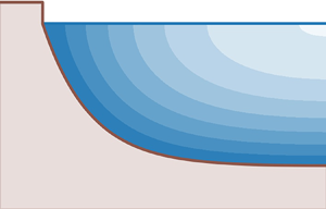
Marche (Reference Marche2007) proposed an improved version of the two-dimensional, shallow-water equations, which accounts for the horizontal flux of momentum in an inertial, non-stationary flow. To our knowledge, the horizontal flux of momentum due to viscosity, as represented in this model, has never been tested per se. In the present paper, we consider a simple configuration in which this can be done, and which is relevant for laminar rivers: a steady, viscous flow that is uniform downstream (figure 1). In this idealized configuration, the velocity aligns with the channel, and we can often derive an analytical expression for it (or at least a simple numerical solution). We take advantage of this simplicity to propose a new expression for the viscous flux of momentum across a shallow, laminar flow (§ 2), and compare it with the exact, two-dimensional flow it should approximate (§ 3). In this simplified context, we find that the new expression is more reliable than that of Marche (Reference Marche2007) (Appendix A). Because it inherits the non-locality of the Stokes flow it approximates, the equation we propose accounts surprisingly well for the flow near the bank of a channel (§ 4).

Figure 1. Typical flow configuration and notations. Flow is along the  $x$ direction, which is inclined with respect to horizontal. Free surface is flat (
 $z=0$), and inclined downstream with slope
  $S$. Blue lines: fluid. Brown shading and dots: solid, impervious substrate.
2. Momentum balance
Rivers are turbulent, and so are most of their laboratory analogues (Métivier et al. Reference Métivier, Lajeunesse and Devauchelle2017). Some experimental flumes, however, are small enough, and the fluid they carry viscous enough, for the flow to remain laminar (Seizilles et al. Reference Seizilles, Devauchelle, Lajeunesse and Métivier2013; Abramian et al. Reference Abramian, Devauchelle and Lajeunesse2020). Provided their path does not bend too much, we are left with a two-dimensional Poisson equation to account for the viscous diffusion of momentum across the flow (§ 2.1). Integrated vertically, this equation becomes a one-dimensional equation (§ 2.2) which, in its simplest form, yields the classical lubrication approximation (§ 2.3). Finally, in § 2.4, we add the contribution of the cross-wise stress to this approximation.
2.1. Continuity equation for a Poiseuille flow
We consider the laminar flow of figure 1, whose unidirectional velocity lies along the  $x$ axis. This configuration implies that the channel's bed, and thus the flow, does not vary in the
  $x$ direction at all. Of course, such an idealized setting can only be an approximate representation of the actual flow, valid when the latter varies only weakly along the
  $x$ direction.
To formalize this assumption, we call  $\mathcal {L}$ the cross-wise extent of the channel (
 $y$ axis), and
  ${\mathcal {L}}_s$ the characteristic length over which the bed changes downstream (
 $x$ axis). When the ratio
  ${\mathcal {L}}/{\mathcal {L}}_s$ is small enough, we may treat the flow as streamwise invariant, and represent it with its only component,
  $u(y,z)$. We use this approximation from now on. Under this assumption, the Stokes equation reduces to
 \begin{equation} \nu \nabla^2 u + g S = 0, \end{equation}
where  $\nu$ is the kinematic viscosity of the fluid,
  $g$ the acceleration of gravity and
  $S$ the downstream slope of the channel (the sine of the angle it forms with the horizontal). The Laplacian operator,
  $\nabla ^2$, applies only to directions orthogonal to the flow, that is,
  $y$ and
  $z$.
$z$.
A convenient consequence of our initial assumption that the flow is invariant along the  $x$ axis is that its free surface is also invariant. This assumption is very limiting: it precludes any free-surface wave and, in fact, any pressure gradient other than hydrostatic. In short, it limits the present theory to two-dimensional Poiseuille flows. This, we argue, is nonetheless a rich class of systems, to which the straight laminar rivers of Abramian et al. (Reference Abramian, Devauchelle and Lajeunesse2020) belong.
We further neglect surface tension, and any other stress on the free surface. Unlike the unidirectional-flow assumption, this hypothesis could well be relaxed in the present framework but, to keep our problem simple, we here assume that the free surface is horizontal (more exactly, it belongs to the  $(x,y)$ plane). We then place the origin on the free surface, which thus corresponds to
  $z=0$. Accordingly,
 \begin{equation} \frac{\partial u}{\partial z} = 0\quad \mbox{for}\ z = 0. \end{equation}
Finally, we treat the bed as an impervious wall, where the velocity of the fluid vanishes
 \begin{equation} u = 0 \quad \mbox{for}\ z ={-}D(y), \end{equation}
where  $D(y)$ is the flow depth. This assumption is only a rough approximation of reality when the bed is made of a granular sediment, into which the velocity profile can penetrate. One could account for this penetration by allowing some slip at the porous surface (Beavers & Joseph Reference Beavers and Joseph1967). Similarly, in the context of flowing ice, a slippery bed surface would also translate into a Robin boundary condition (Schoof & Hewitt Reference Schoof and Hewitt2013). Here, for simplicity, we just keep (2.3) until Appendix C.2, where we touch upon the subject of slip.
Equation (2.1), and the associated boundary conditions (2.2) and (2.3), represent a Nusselt flow down a channel of arbitrary section (Benjamin Reference Benjamin1957). They sometimes have closed-form solutions, for instance when the channel is elliptic (§ 3.1), but in general they do not, and one needs to approximate their solution with a series expansion, or some other numerical method (§§ 3.2 and 3.4). Here, (2.1) to (2.3) serve as our reference, against which we can evaluate the new shallow-water approximation we introduce in § 2.4. In that sense, we refer to them as ‘the exact equations’ although, of course, they are but an approximation of the actual flow.
2.2. Integrated momentum balance
Integrating the exact momentum balance (2.1) over a vertical section, and invoking the free-surface boundary condition (2.2), we find
 \begin{equation} \nu \int_{{-}D}^0 \frac{\partial^2 u}{\partial y^2} \mathrm{d} z - \frac{\tau_z}{\rho} + g S D = 0, \end{equation}
where  $\rho$ is the density of the fluid and
  $\tau _z$ is the vertical component of the viscous stress on the bed's surface. In a Newtonian fluid, the latter reads
 \begin{equation} \tau_z = \rho \nu \left. \frac{\partial u}{\partial z} \right|_{z={-}D}. \end{equation}
A more usual notation for  $\tau _z$ would be
  $\tau _{xz}$, but in the present context the shorthand notation
  $\tau _z$ leaves no ambiguity.
To rewrite the integral in (2.4), we first remember that the free surface is flat and, accordingly, differentiate only the lower bound of the integral along the bed's surface
 \begin{equation} \int_{{-}D}^0 \frac{\partial^2 u}{\partial y^2} \mathrm{d} z = \frac{\partial}{\partial y } \int_{{-}D}^0 \frac{\partial u}{\partial y} \mathrm{d} z - \frac{\partial D}{\partial y} \left.\frac{\partial u}{\partial y} \right|_{z={-}D}. \end{equation}
We then use the no-slip boundary condition (2.3) which, again, we differentiate across the stream
 \begin{equation} \left. \frac{\partial u}{\partial y} \right|_{z={-}D} = \frac{\partial D}{\partial y} \left. \frac{\partial u}{\partial z} \right|_{z={-}D}. \end{equation}
The above relation tells us that the vertical component of the shear stress,  $\tau _z$, its cross-wise counterpart,
  $\tau _y$, and the norm of the shear stress,
  $\tau$, are all related to each other through
 \begin{equation} \tau\equiv \sqrt{ \tau_y^2 + \tau_z^2 } = \tau_z \sqrt{ 1 + \left( \frac{\partial D}{\partial y} \right)^2 }. \end{equation}
Since the above relation is exact, and since the shape of the channel,  $D(y)$, is a given of the problem, we can treat
  $\tau _z$ and
  $\tau$ as equivalent quantities. Hereafter, based on this observation, we will use
  $\tau _z$ or
  $\tau$ interchangeably, depending on which one is more convenient, or more telling.
The no-slip boundary condition (2.3) also allows us to write
 \begin{equation} \int_{{-}D}^0 \frac{\partial u}{\partial y} \mathrm{d} z = \frac{\partial}{\partial y} \int_{{-}D}^0 u \, \mathrm{d} z, \end{equation}
which, together with (2.7), we inject in the vertical integral of the Poisson equation (2.4). We finally find
 \begin{equation} \rho \nu \frac{\partial^2}{\partial y^2} (U D) - \tau_z \left(1 + \left( \frac{\partial D}{\partial y}\right)^2 \right) + \rho g S D = 0, \end{equation}
where we have defined the vertically averaged velocity  $U$ as
 \begin{equation} U = \frac{1}{D} \int_{{-}D}^0 u \, \mathrm{d} z. \end{equation}
The one-dimensional momentum balance (2.10) follows from (2.1) to (2.3) without any additional assumption – in that sense, it is exact. The first term is the divergence of the cross-stream flux of momentum, the second one is the momentum lost to friction with the bottom, and the last one is the source of downstream momentum, powered by gravity.
A similar balance could be established without assuming that the free surface is flat, and the flow unidirectional; it would then explicitly couple the transverse flow to the deformations of the free surface. Assuming the flow to be unidirectional thus simplifies (2.10), but it makes the present theory unable to handle bedforms (unless they are invariant along the  $x$ direction, § 3.3).
Even in the simple form of (2.10), the integrated momentum balance is incomplete: it involves two unknown functions of the cross-wise coordinate  $y$ (the shear stress
  $\tau _z$ and the average velocity
  $U$). This was to be expected, since we just integrated the Poisson equation vertically, without trying to solve it. At this point, unfortunately, we can postpone no further resorting to approximation.
2.3. Classical lubrication approximation
The lubrication theory relies on the flow being shallow. To quantify this statement, we define a small parameter,  $\epsilon$, as the aspect ratio of the channel's cross-section
 \begin{equation} \epsilon = \frac{\mathcal{H}}{\mathcal{L}}, \end{equation}
where  $\mathcal {H}$ is the characteristic depth of the channel. Upon rescaling of the
  $y$ and
  $z$ coordinates with
  $\mathcal {L}$ and
  $\mathcal {H}$ respectively, the cross-wise derivative in the exact Poisson equation (2.10) is multiplied by
  $\epsilon ^2$ (Appendix B.1). Assuming
  $\epsilon$ is small, one can thus neglect the flux of momentum that viscosity transfers across the flow. The classical lubrication approximation is based on this idea.
Neglecting the cross-wise flux of momentum in the Poisson equation (2.10), we find the classical velocity profile of a Poiseuille flow,
 \begin{equation} u = \frac{ 3 U }{ 2 D^2 } (D^2 - z^2), \end{equation}
where the vertically averaged velocity  $U$ is related to the vertical component of the shear stress on the bed,
  $\tau _z$, through
 \begin{equation} \tau_z = \frac{3 \rho \nu U}{D}. \end{equation}
Since the momentum that gravity delivers to the fluid does not propagate in the cross-wise direction, the surface of the bed needs to absorb it all, and thus
 \begin{equation} \tau_z = \rho g S D. \end{equation}
Equations (2.13) to (2.15) are exact when the channel is perfectly flat and infinitely wide ( $\epsilon =0$). They are also the leading-order terms in the expansion of the flow as a power series in
  $\epsilon$ (Appendix B.1). The gist of the classical lubrication approximation is to assume that these leading-order equations provide a decent approximation of the flow when
  $D$ varies slowly across the channel. In the case of a unidirectional flow in a straight channel, this simply translates into (2.13) to (2.15) – only with varying coefficients
  $U(y)$ and
  $D(y)$.
The main advantage of this approach is its wonderful simplicity. The cost of this simplicity, however, is that the resulting velocity  $U(y)$ violates the momentum balance (2.10) at order
  $\epsilon ^2$. In the next section, we improve the lubrication approximation by proposing a representation of the flow that satisfies it exactly.
2.4. Revised lubrication theory
We would like to improve the classical lubrication approximation so that it accounts for the momentum balance, while keeping the problem low-dimensional. Our objective is to predict the distribution of shear stress on the channel's bed better than the classical theory, at a small computational cost. This endeavour is in line with the work of Marche (Reference Marche2007), although here we limit ourselves to the configuration of a steady flow in a straight channel.
To refine an approximate theory based on a series expansion, it is customary to look for the next term in the expansion – here, the term of order  $\epsilon ^2$. Appendix B.1 is devoted to this standard method which, as expected, yields a correction to the classical lubrication approximation. Here, however, we propose a less conventional method based on the ansatz of the classical theory, in the hope of obtaining a more flexible representation of the flow. The expansion of Appendix B.1 will be our touchstone: to qualify as progress, the revised theory should be correct at least up to order
  $\epsilon ^2$.
The reasoning we propose does not have the mathematical rigour of an order expansion, but it is extremely simple. It relies on the observation that it is only by enforcing (2.15) that we make (2.14) violate the momentum balance (2.10). In itself, (2.14) only links the average velocity,  $U$, with the shear stress on the bed,
  $\tau _z$, when the vertical velocity profile is parabolic (2.13). In short, (2.14) just relates two unknowns, and thus spares one degree of freedom.
It is, we believe, in the spirit of the shallow-water approximation to make the most of this freedom, by dropping (2.15) while keeping (2.14). Specifically, we use the shape of the vertical profile (2.13) as an ansatz which relates the average velocity,  $U$, to the shear stress,
  $\tau _z$, through (2.14). In practice, this means substituting (2.14) into the momentum balance (2.10), which then reads
 \begin{equation} \frac{1}{3} \frac{\mathrm{d}^2}{\mathrm{d}y^2} ( D^2 \tau_z ) -\left( 1 + \left(\frac{\mathrm{d} D}{\mathrm{d}y} \right)^2 \right)\tau_z + \rho g S D = 0. \end{equation}
This second-order ordinary differential equation is the substitute we propose for (2.15). Its only unknown is  $\tau _z$. The flow depth,
  $D(y)$, although it appears at various orders of derivation, is the given boundary to which the flow adjusts.
Equation (2.14), which relates the friction on the bottom to the average velocity, is essentially a friction law. The approximate momentum balance (2.16) depends on this friction law, and it is therefore just as reliable as the latter (Appendix C).
Before we set off to investigate the validity of (2.16), we first acknowledge some of its encouraging features. First, it becomes (2.15) again over a flat bed – as it should. More interestingly, it is equivalent to the exact Poisson equation (2.1) up to order  $\epsilon ^2$, which ensures that it is an improvement upon the classical (zeroth-order) theory (Appendix B.2). Finally, that it is a differential equation instead of an algebraic one is only slightly inconvenient, since (2.16) is linear in
  $\tau _z$, and therefore amenable to classical resolution methods. We still need to check, however, that this equation is worth the effort of solving it.
The classical lubrication theory merely equates the vertical component of the shear stress,  $\tau _z$, with the momentum that gravity injects into a vertical slice of the flowing fluid,
  $\rho g S D$. Thus, not only does it neglect the transfer of momentum across the stream, but also approximates the flux of momentum into the bed with its vertical component,
  $\tau _z$. The revised theory does neither. Indeed, integrating (2.16) between two points across the stream, say
  $y_1$ and
  $y_2$, and invoking (2.7), we find
 \begin{equation} \left[\frac{1}{3} \frac{\mathrm{d}}{\mathrm{d}y} ( D^2 \tau_z ) \right]_{y_1}^{y_2} - \int_{s(y_1)}^{s(y_2)} \tau \, \mathrm{d}s + \rho g S \int_{y_1}^{y_2} D \, \mathrm{d}y = 0, \end{equation}
where  $s$ denotes the arclength along the bed's surface (this change of variable is based on (2.8)). The first term in the above equation represents the cross-wise flux of momentum, the second one is the total momentum transferred to the bed and the last one is the momentum injected into the flow by gravity. The first term is an approximation, whereas the two others are exact. Regardless of the correctness of the first term, however, the three of them balance each other exactly – provided
  $\tau _z$ fulfils (2.16).
In other words, (2.16) is a proper continuity equation for momentum. The downstream momentum that gravity constantly supplies to the flow is either transmitted to the bed, or distributed sideways by viscosity. To close this balance, therefore, one needs to account for the momentum that is transferred across the stream. The value of the shear stress at a specific location on the bed thus depends on the shape of the entire channel. In mathematical terms, (2.16) is non-local – a property inherited form the Poisson equation (2.1).
As encouraging as it may seem, the above features do not guarantee that (2.16) is a better approximation of the flow than the expansion of Appendix B.1, which is a local, algebraic equation: both are correct up to order  $\epsilon ^2$. We devote the next section to testing (2.16) in a variety of – hopefully instructive – configurations.
3. Test cases
Once the cross-section of the channel is fixed by choosing  $D(y)$, we can solve (2.16), and therefore estimate the bottom shear stress,
  $\tau _z$, according to the revised lubrication theory. To evaluate how accurate this approximation is, we need to solve the exact (2.1), and compute the associated shear stress. When the channel's shape is suitably simple, there are closed-form solutions of the Poisson equation (§ 3.1). In a rectangular channel, we can still expand the exact solution into a series (§ 3.2), but when the channel's bottom is corrugated, we need to resort to linearization (§ 3.3) or finite elements (§ 3.4) to solve the problem of reference.
3.1. Exact solutions
3.1.1. Wedge flow
Let us first consider a Poiseuille flow in a wedge (figure 2a). This configuration may represent a river bank, where the water surface ( $z = 0$) intersects the bed (
 $z = -\mu y$). Mathematically, this problem is ill posed, since it lacks a boundary condition on the open side of the wedge. We could fix such a condition, of course, but this would rule out any closed-form solution. Close enough to the corner, anyway, we expect that the flow velocity will be insensitive to the boundary condition, and will thus behave like
 \begin{equation} u =\frac{gS}{\nu} \frac{( \mu y - z )( \mu y + z )}{ 2( 1 - \mu^2 ) } =\frac{gS}{\nu} \frac{ D^2 - z^2 }{ 2( 1 - \mu^2 ) }, \end{equation}
an expression that satisfies (2.1) exactly (except for  $\mu =1$, § 4). Based on this expression, the shear stress the flow exerts on the bed's surface is proportional to the water depth,
  $\mu y$
 \begin{equation} \tau_z = \frac{ \rho g S \mu y }{ 1 - \mu^2 }. \end{equation}
We now need to evaluate the revised lubrication approximation against this result. This is straightforward: as it turns out, (3.2) is also a solution of (2.16). This is not true for the classical lubrication approximation since, in a wedge, (2.15) reads  $\tau _z = \rho g S \mu y$. The revised theory thus proves an improvement in this case, at least when the bank is not too steep (
 $\mu <1$; § 4 is devoted to
  $\mu \geq 1$).

Figure 2. Exact solutions to both the two-dimensional Poisson equation (2.1), and the revised lubrication theory, (2.16). Aspect ratio is preserved. Blue shading show velocity contours. The width of the channel is  $W$. (a) Wedge flow, (3.1) with
  $\mu = 1/3$. The flow extends to
  $y \rightarrow + \infty$ on the right-hand side. (b) Elliptic channel, with aspect ratio
  $R = 3.5$, (3.4).
3.1.2. Elliptic channel
We now turn our attention to a better-defined problem, and consider an elliptic channel of width  $W$, and aspect ratio
  $R$ (figure 2b), the depth of which reads
 \begin{equation} D = \frac{1}{R} \sqrt{ W^2 - 4 y^2 }. \end{equation}
The corresponding solution of the Poisson equation (2.1) is (Boussinesq Reference Boussinesq1868, p. 388)
 \begin{equation} u = \frac{g S \left(W^2 - 4 y^2 - (Rz)^2\right)}{2 \nu \left( R^2 + 4 \right)}. \end{equation}
Differentiating the above equation, we find the expression of the vertical component of the shear stress on the bed's surface
 \begin{equation} \tau_z = \frac{\rho g S R \sqrt{W^2-4y^2}}{R^2+4}. \end{equation}
Again, this expression happens to be an exact solution to (2.16) – the approximation could not be more accurate. In fact, the velocity field associated with the revised lubrication approximation, namely
 \begin{equation} u = \frac{D}{2\rho \nu}\left( R^2 - \left( \frac{z}{D} \right)^2 \right) \tau_z, \end{equation}
is the exact solution of the original Poisson equation. This result, which seems coincidental at first, appears inevitable after careful consideration. Indeed, in an elliptic channel, the vertical velocity profile of the exact solution is parabolic, making the ansatz of the revised theory a perfect representation of the flow. Conversely, the classical lubrication theory overestimates the shear stress by a factor of  $(R^2 + 4)/R^2$.
Although limited to channels of specific shapes, the perfect match between the revised theory and the reference problem is encouraging. In particular, it is remarkable that the revised theory works so well in an elliptic channel of arbitrary aspect ratio, where the hypothesis of a shallow flow does not hold at all. In the next section, we test the revised theory under even worse conditions.
3.2. Rectangular groove
Let us, for a change of context, imagine a straight microfluidic groove engraved into a solid substrate, with a rectangular cross-section (figure 3a,b). The flat bottom of the channel, of course, would be no challenge for the lubrication theory, were it not for the two sidewalls, where the no-slip boundary condition applies. There is no closed-form solution of the Poisson equation in a channel of rectangular cross-section, but there exists a solution in the form of an infinite series (e.g. White Reference White1991)
 \begin{equation} u = \frac{4 g SW^2}{\nu {\rm \pi}^3}\sum_{k=1,3,5,\ldots}^{\infty} \frac{({-}1)^{(k-1)/2}}{k^3}\left(1 - \frac{\cosh(k{\rm \pi} z/W)}{\cosh(k{\rm \pi} D/W)}\right)\cos \left(\frac{k{\rm \pi} y}{W} \right), \end{equation}
where  $W$ is the width of the channel, and
  $D$ its (uniform) depth. In this sum, the index
  $k$ can be interpreted as a dimensionless wavenumber. Differentiating the above expression with respect to
  $z$ yields the bottom shear stress
  $\tau _z$ with arbitrary precision (blue line in figure 3(c,d),
  $\tau$ is exactly
  $\tau _z$ in this case). As expected, we find that viscosity conveys the influence of the walls across the flow, making the bottom shear stress reach a maximum in the middle of the channel.

Figure 3. Laminar flow in a rectangular groove. (a,b) Streamwise velocity (blue shading), according to series expansion (3.7) truncated at  $k=99$. Aspect ratio is preserved. (c,d) Intensity of flow-induced shear stress on bottom (
 $\tau$). Solid blue: series expansion (3.7) truncated at
  $k=99$, for reference. Dash-dotted grey: classical lubrication approximation (2.14). Dashed orange: present theory (3.8). Channel aspect ratio is
  $W/D=5$ (a,c) and
  $W/D=1$ (b,d).
The classical lubrication theory, in the form of (2.15), cannot account for the no-slip boundary condition at the sidewalls. In fact, according to this approximation, the shear stress just remains constant across the entire channel. As a consequence, although this constant is a reasonable estimate of the shear stress far away from the walls, the classical theory fails entirely in their neighbourhood (grey line in figure 3c,d).
Equation (2.16), conversely, requires two boundary conditions, which allows us to fix the velocity of the flow along the side walls: (2.3) translates the no-slip condition into  $\tau _z=0$ in
  $y=\pm W/2$. The uniform depth of the channel makes this problem a textbook exercise, whose solution is
 \begin{equation} \tau_z =\rho g S D
\left( 1 - \frac{\cosh ( \sqrt{3} y/ D )}{\cosh
( \sqrt{3} W/(2D) )} \right).
\end{equation}
\begin{equation} \tau_z =\rho g S D
\left( 1 - \frac{\cosh ( \sqrt{3} y/ D )}{\cosh
( \sqrt{3} W/(2D) )} \right).
\end{equation}
We find that this expression is a much better approximation of the actual shear stress than the constant of the classical theory (orange line in figure 3c,d). In particular, the sidewalls affect the flow over a distance comparable to the channel's depth. In a channel of aspect ratio  $W/D=5$ (figure 3a,c), the largest error of the present theory is less than 10 % of the average shear stress (the average error is approximately 2 %). Combining (3.8) with the ansatz (2.13), and integrating the result across the channel, yields an estimate for the total discharge of a rectangular microfluidic groove; we find that this estimate lies within less than 3 % of the actual value, whereas the classical theory is more than 30 % off.
The revised lubrication theory relies on the friction law (2.14), which derives from the assumption that the flow profile is essentially that of a Nusselt film. Near the walls, however, this hypothesis breaks down, because the walls cause the profile to depart from its parabolic shape, thus affecting the friction law (Appendix C.1). It turns out, however, that the vicinity of a wall also lessens the contribution of bottom friction to the momentum balance. As a result, the friction term gets wrong where it does not matter much, which bolsters the validity of the revised lubrication theory near a wall.
In a narrower channel ( $W/D=1$, figure 3b,d), we expect both the classical and the revised theories to fail. Indeed they do, but not to the same extent. The revised theory underestimates the discharge by approximately 12 %, whereas the classical theory overestimates it by a factor of almost 5. As visible on figure 3(d), this difference results from the ability of the revised theory to account for friction along the sidewalls (Appendix B.1).
The non-locality of (2.16) comes at a cost but, as this case illustrates, it keeps the momentum balance under control. This, we argue, is why the revised theory is more reliable than the classical theory.
3.3. Linear perturbation
We now consider a channel of infinite width, the bottom of which is perturbed with a sinusoidal corrugation of infinitesimal amplitude (figure 1). In tune with our initial assumption, the flow remains invariant in the  $x$ direction; the crests and troughs of the corrugation, therefore, are aligned with the flow velocity. Mathematically,
 \begin{equation} D = D_0 + Re \left( {D}^{* }_1 \exp \left( \frac{\textrm{i}ky}{D_0} \right) \right), \end{equation}
where  ${D}^{* }_1$ is the (possibly complex) amplitude of the perturbation (
 $| {D}^{* }_1|\ll D_0$),
  $D_0$ is the unperturbed depth of the channel and
  $k$ is the dimensionless wavenumber of the perturbation (the corresponding wavevector is aligned with the
  $y$ axis). When the perturbation vanishes, the bottom shear stress,
  $\tau _{z,0}$, is related to
  $D_0$ through (2.15).
Abramian et al. (Reference Abramian, Devauchelle and Lajeunesse2019a) investigated the stability of a similar perturbation when the bed over which the fluid flows is made of mobile sediment. Since it is the flow-induced shear stress that drives sediment transport in this case, one essential step of their analysis was to linearize the exact Poisson equation (our (2.1)), and to analytically solve the resulting linear problem. Their (3.7) will serve as our reference; in the present notations, it reads
 \begin{equation} \tau_z = \tau_{z,0} \left( 1 + \left( 1 - k \tanh{k} \right) Re \left( \frac{ {D}^{* }_1}{D_0} \exp \left( \frac{\textrm{i}ky}{D_0} \right) \right) \right). \end{equation}
The above equation indicates that the shear stress is in phase with the sinusoidal perturbation; its extrema lie where the perturbation's are. More remarkably, the sign of the shear-stress perturbation depends on the wavelength of the bed perturbation (blue line in figure 4). When this wavelength is large enough ( $k< k_c$, where
  $k_c\approx 1.20$), the shear stress is at its highest in the troughs, where the flow is deeper – in tune with the classical lubrication theory. On the contrary, when the perturbation's wavelength is short enough (
 $k>k_c$), the crests of the corrugation find themselves more exposed to the bulk of the flow, and are therefore subjected to a stronger stress. In other words, the crests then shield the troughs, which collect a smaller share of the flow's momentum. This mechanism, the signature of the Laplacian in (2.1), is essentially the same as the shadowing that sets the shape of diffusion-limited aggregates (Witten & Sander Reference Witten and Sander1981) and causes the Saffman–Taylor instability (Saffman Reference Saffman1986). It is crucial to the stability analysis of Abramian et al. (Reference Abramian, Devauchelle and Lajeunesse2019a), as it prevents the perturbations with the shortest wavelengths to grow infinitely fast, thus selecting the wavelength most likely to appear in an experiment.

Figure 4. Spectral response of bottom shear stress to a bed perturbation of infinitesimal amplitude. Blue line: linearized two-dimensional solution (3.10) for reference (Abramian et al. Reference Abramian, Devauchelle and Lajeunesse2019a). Blue dot: critical wavenumber  $k_c\approx 1.20$. Dash-dotted grey line: classical lubrication approximation (3.11). Orange dashed line: present theory (3.13).
The classical lubrication theory cannot account for this phenomenon. Indeed, it directly relates the shear stress to the amplitude of the perturbation, regardless of its wavelength
 \begin{equation} \frac{ \tau_z - \tau_{z,0} }{ \tau_{z,0} }= \frac{ D - D_0 }{ D_0 }=Re \left( \frac{ {D}^{* }_1}{D_0} \exp \left(\frac{\textrm{i}ky}{D_0} \right) \right). \end{equation}
In the Fourier space, this translates into a flat response (grey line in figure 4). The present theory, on the other hand, is designed to account for the cross-wise flux of momentum. To compare it with (3.10), we first linearize (2.16) about a horizontal bed. We find
 \begin{equation} \frac{D_0^2}{3} \frac{\mathrm{d}^2}{\mathrm{d}y^2} \frac{\tau_{z,1}}{\tau_{z,0}} + \frac{2 D_0}{3} \frac{\mathrm{d}^2 D_1}{\mathrm{d}y^2} - \frac{\tau_{z,1}}{\tau_{z,0}} + \frac{D_1}{D_0}= 0, \end{equation}
where  $D_1$ and
  $\tau _{z,1}$ are the linear corrections to the base state of the flow depth and the shear stress, respectively. Applying a Fourier transform to the above expression, we get
 \begin{equation} \frac{ {\tau}^{* }_{z,1}}{\tau_{z,0}} = \frac{1 - 2k^2/3}{1 + k^2/3} \frac{ {D}^{* }_1}{D_0}, \end{equation}
where the symbol  $\, { }^{* }\,$ denotes the Fourier amplitude of the quantity it decorates. For long wavelengths (
 $k\ll 1$), this expression correctly approximates the exact linear result (3.10), but departs from it as the wavelength of the perturbation approaches the flow depth (
 $k \sim 1$) (orange line in figure 4). Before this happens, however, the present theory accounts for the sign change of the shear stress near
  $k_c$, which it estimates at
  $\sqrt {3/2}\approx 1.22$ – within 2 % of the true value.
The quality of the present approximation turns out to be surprisingly good. In a fashion quite typical of shallow-water theories, it works better than it should. Indeed, if we expand (3.12) and (3.13) into Taylor series, they match up to order  $k^4$ only (odd orders all vanish); reasonably good, perhaps, but insufficient to account for the sign change in figure 4, since this well-controlled, but truncated, expansion fails to ever change sign, unlike the original equation (3.13). In short, it seems we can push the revised lubrication theory beyond where a well-controlled order expansion endorses it – at our own risks, of course.
Taking such risks, however, would be of little use if the revised lubrication theory were to fail beyond the linear regime, in which the two-dimensional equation it approximates can be solved relatively easily. The next section addresses this point.
3.4. Finite-amplitude corrugation
The revised lubrication theory fairly reproduces the results of the linearized, two-dimensional Poisson equation (§ 3.3). We now perturb a flat bed with a corrugation of finite amplitude, thus precluding any linearization of the problem. To test the present theory, we need a reference, which analytical calculations can no longer provide. Instead, we solve (2.1) in a corrugated channel with finite elements (FreeFem++, Hecht (Reference Hecht2012), blue shading in figure 5a,b). Upon differentiation with respect to  $y$ and
  $z$, these numerical simulations yield an approximation of the flow-induced shear stress on the bed (blue line in figure 5c,d).

Figure 5. Laminar flow above a corrugated bottom (a,b), and associated shear stress on the bed (c,d). Blue shading in (a,b) shows two-dimensional velocity (2.1) (finite-element simulations, arbitrary units). Flow is towards viewer. Aspect ratio is preserved. Solid blue lines in (c,d): shear stress from finite-element simulations. Dotted brown line: linearized two-dimensional flow (3.10) (Abramian et al. Reference Abramian, Devauchelle and Lajeunesse2019a). Dashed orange lines: present theory (2.16) (numerical solution): (a,c)  $k=6$ and
  $D^*_1 = 0.03 D_0$; (b,d)
  $k=0.6$ and
  $D^*_1 = 0.7 D_0$.
We consider two configurations, in which the corrugations differ in amplitude and wavelength. In the first case, the wavelength of the corrugation is shorter than the flow depth ( $k=6$), while its amplitude remains small, albeit not vanishing (
 ${D}^{* }_1= 0.03 D_0$, figure 5a,c). We expect both the classical lubrication theory and the present theory to fail in this case, due to the short wavelength of the perturbation. In the second case, the wavelength is significantly larger than the flow depth (
 $k=0.6$), while the amplitude is comparable to the depth (
 ${D}^{* }_1=0.7D_0$, figure 5b,d). It is in such a flow configuration that the revised theory could prove useful.
In the first case, the amplitude of the perturbation is small enough (with respect to depth) for the linearized theory of § 3.3 to provide a good approximation of the shear stress (dotted brown line in figure 5c). This is not true, however, for the classical lubrication theory, which wrongly locates the maxima of the shear stress in the troughs (dashed grey line). This was to be expected, since our choice of wavenumber is far beyond  $k_c$, the wavenumber above which the crests shield the troughs (§ 3.3). The revised lubrication theory, in the form of a numerical solution of (2.16), does a little better, since it locates the maxima correctly, but the amplitude of its prediction is off. For very short wavelengths, therefore, the only alternative to the exact Poisson equation remains the linear, two-dimensional theory.
Conversely, in the second case, the amplitude of the perturbation is too large (with respect to depth) for the linear, two-dimensional theory (dotted brown line in figure 5d). Moreover, its wavelength is too short for the classical lubrication approximation (dash-dotted grey line). The revised lubrication theory, on the other hand, handles this case gracefully: the numerical solution of (2.16) matches the finite element simulation of the full two-dimensional problem everywhere within 2.3 % of the average stress (dashed orange line). Equation (2.16) thus represents accurately the diffusion of momentum across the flow, which makes it a convenient alternative to the Poisson equation in this case.
This encouraging result would not survive a significant shortening of the perturbation's wavelength, that is, a reduction of the aspect ratio of the flow. As it is, however, the periodic configuration of figure 5(b) evokes a series of channels of aspect ratio  ${\rm \pi} D_0/( k {D_1}^{* } )\approx 7.5$ – a value comparable to that of laboratory rivers (Seizilles et al. Reference Seizilles, Devauchelle, Lajeunesse and Métivier2013). In the next section, inspired by these experiments, we consider a configuration in which the corrugation and the free surface intersect, thus forming the bank of a river.
4. Flow along a corner
In § 3.1.1, we noted that the analytical solution of the Poisson equation in a wedge diverged at a special value of the wedge angle, namely  $\mu =1$ – and we quickly moved on. We now consider this problem in details. In fact, this is a typical difficulty with any shallow-water or lubrication theory: when the bottom of the flow reaches the free surface, their intersection creates a singularity. This singular point, or line, often becomes an issue when one numerically simulates a sheet flow over a rough bed that can protrude through the fluid's surface (Delestre et al. Reference Delestre, Cordier, Darboux, Du, James, Laguerre, Lucas and Planchon2014).
In this section, true to the form of the paper, we consider a simpler version of this problem: the laminar flow of a viscous fluid in a channel with a sharp corner (figure 6). At the bank, the flow forms a wedge bounded by the bed and the free surface, which intersect each other at an angle  $\beta$ (the slope of the bank is
  $\mu = \tan \beta$). Away from the corner, the bottom gradually returns to the horizontal, until it reaches an axis of symmetry (dashed blue line on figure 6). The assumption, here, is that the flat part of the bed, and the exact location of the axis of symmetry, do not really matter to the flow near the corner.

Figure 6. Laminar flow in a channel with a sharp corner (finite-element simulation). Channel shape corresponds to (4.4). The tangent of the corner angle is  $\mu$. Blue shading: flow velocity.
We begin with our usual reference, the Poisson equation (2.1), for which we find a variety of asymptotic behaviours near the corner (§ 4.1). We then try to identify the same regimes in the revised lubrication theory (§ 4.2). The classical lubrication theory, of course, is irrelevant for this problem, since it assumes that the fluid's velocity is proportional to the local flow depth, and therefore undergoes no transition when  $\mu =1$.
4.1. Poisson equation
The Poisson equation (2.1) is linear and non-homogeneous. It is thus convenient to decompose its solutions into the sum of a homogeneous solution and a special solution. Dropping the source term of the Poisson equation, we are left with the Laplace equation,
 \begin{equation} \nabla^2 u = 0, \end{equation}
to which we can find solutions in the form of analytical functions of the complex variable  $\omega = y + \textrm {i} z$ (the bank is located at
  $\omega =0$). Then, we will need to find a special solution to the original Poisson equation. Unless
  $\mu =1$, this will simply be (3.1), the solution we encountered in § 3.1.1.
4.1.1. Homogeneous solution
In a corner of angle  $\beta$, there exists a power-law solution to the Laplace equation (4.1) that satisfies boundary conditions (2.2) and (2.3). Namely,
 \begin{equation} u^{(h)} = C \, Re [ \omega^{ {\rm \pi}/( 2 \beta)} ], \end{equation}
where  $\omega = y + \textrm {i} z$ is the complex coordinate, and
  $C$ is a positive constant with physical dimensions (Polubarinova-Kochina Reference Polubarinova-Kochina1962). Differentiating the above expression, we get the vertical component of the shear stress,
  $\tau _z$
 \begin{equation} \tau_z^{(h)} = C' y^{ {\rm \pi}/(2\beta) - 1}, \end{equation}
where  $C'$ is another positive constant. The exponent of the above expression is already an indication that a slope of
  $\mu =1$ might be a special value. Indeed, when
  $\beta = {\rm \pi}/4$, the exponent of the above expression is exactly 1 – the exponent of the special solution (3.2). Motivated by this observation, we now compare the homogeneous solution (4.3) with the special solution.
4.1.2. Shallow bank ( $\mu <1$)

When the bank is shallow enough ( $\mu <1$ or equivalently
  $\beta < {\rm \pi}/4$), the special solution (3.1) remains finite and positive, and thus physically acceptable. In a given channel, such as those of figure 6, the actual flow is then the sum of this special solution and a homogeneous solution (4.2), the prefactor of which,
  $C$, adjusts to the far field, that is, to the overall shape of the channel.
Provided the corner's angle,  $\beta$, is less than
  ${\rm \pi} /4$, the exponent of the homogeneous solution (4.3) is larger than one, and therefore larger than that of the special solution. As a consequence, the special solution dominates the flow in the bank's neighbourhood (
 $\omega \rightarrow 0$), and the shear stress is well approximated by (3.2), in which there is no parameter that adjusts to the far field.
To compare this asymptotic behaviour with numerical simulations, we first devise a concrete example of a channel with a bank slope of  $\mu$. We expect that, apart from the bank, the general shape of the channel will not alter the asymptotic behaviour of the flow in the corner. To fix the channel's shape, we arbitrarily define its cross-section as
 \begin{equation} D = D_m \frac{\cosh( \mu ( y/D_m - R/2 ) ) - \cosh( \mu R/2 )}{\sinh( \mu R/2 )}, \end{equation}
where  $D_m$ sets the depth of the channel, and
  $R$ sets its aspect ratio (figure 6). In practice, we choose
  $R=8$, whereas
  $D_m$ does not matter once the problem is made dimensionless. We then run finite-element simulations in such a channel to numerically approximate the velocity field
  $u$, which is a solution to the Poisson equation (2.1) (blue shadings in figure 6). By differentiating this velocity, we find the shear stress on the bed,
  $\tau _z$. For a shallow bank (
 $\mu <1$), we find good agreement between the numerical solution (solid blue line in figure 7) and the special solution (3.2) (dashed blue line in figure 7), without adjusting any parameter. This shows that, near a shallow bank, the flow is indeed dominated by the special solution, the asymptotic behaviour of which is independent of the rest of the flow (the far field).

Figure 7. Shear stress along the bed of a channel with sharp corner. Solid lines correspond to the finite-element simulations of figure 6. Dashed blue line is (3.2), without any fitted parameter. Dotted brown line is (4.3) with coefficient  $C'$ fitted to finite-element simulation. Dash-dotted orange line: (4.6), with
  $C_b$ arbitrarily set to
  $D_m$.
However, as the bank's angle approaches  $45^{\circ }$ (
 $\mu =1$), (3.1) breaks down, and the flow near the bank takes another form.
4.1.3. Steep bank ($\mu >1$)

When the bank is steep ( $\mu >1$), the special solution (3.2) yields a negative shear stress in the corner – quite unrealistic. This is an indication that, in this case, we cannot neglect the homogeneous solution anymore.
In fact, the homogeneous solution (4.2) takes over the flow near the bank. Mathematically, the exponent of the homogeneous solution (4.2) becomes less than one and, therefore, the homogeneous solution overshadows the special solution (3.2) near the bank ( $\omega \rightarrow 0$). As a consequence, the leading-order term in the velocity field is now a power law with a varying exponent (namely
  ${\rm \pi} /(2\beta )$), which depends on the bank's slope – and so does the shear stress through (4.3). The dependence of an exponent on the shape of the boundary is not unheard of; it is in fact quite typical of the Laplace equation (Polubarinova-Kochina Reference Polubarinova-Kochina1962). That it happens in a viscous flow is reminiscent of the recirculation loops identified by Moffatt (Reference Moffatt1964), although the transition we find here is mathematically simpler.
Again, the finite element simulations match this asymptotic regime near the bank although, this time, we need to fit the constant  $C'$ to the numerical data (dashed and solid brown lines in figure 7). The value of this prefactor, indeed, depends on the shape of the entire channel – the far field matters for the flow along a steep corner, even at leading order.
4.1.4. Intermediate bank ($\mu =1$)

When the slope of the bank is exactly one ( $\beta = {\rm \pi}/4$), finding a special solution of the Poisson equation (2.1) requires more work. One method is to write the solution as the sum of a radially symmetric term that does not match the boundary conditions, with an analytical term that corrects this mismatch. A simple expression for the first is
  $-gS\omega \bar {\omega }/(4\nu )$ (the overbar denotes complex conjugation), which naturally satisfies the free-surface boundary condition, but not the no-slip condition on the channel's bed. We now need to find an analytical function that compensates for this shortcoming. There might be a principled method to do so, but we used trial and error to identify, among the usual suspects of complex analysis (power laws and logarithm), the one that suits our problem, namely:
 \begin{equation} u ={-} \frac{gS}{\nu} \mbox{Re} \left( \frac{ \omega \bar{\omega} }{ 4 } + \frac{\omega^2}{\rm \pi} \log \left( \frac{\omega}{ C_b } \right) \right), \end{equation}
where  $C_b$ is an arbitrary positive constant. This constant relates the flow near the corner to the far field. Unlike for a steep bank (§ 4.1.3), however, this constant plays only a minor role in the neighbourhood of the bank, as
  $\log \omega$ overcomes
  $\log C_b$. This was to be expected, perhaps, in the special case that marks the transition between the shallow bank, for which the far field does not matter, and the steep bank, for which the far field dominates the flow.
Differentiating (4.5) along the  $z$ direction, we finally find an expression for the shear stress near the bank
 \begin{equation} \tau_z \approx{-} \frac{ 2 \rho g S }{\rm \pi} y \log \left( \frac{y}{ C_b } \right). \end{equation}
The finite-element simulations match this peculiar scaling, even when the constant  $C_b$ is arbitrarily set to
  $D_m$ (orange lines in figure 7).
To represent the transition from the shallow-bank asymptotic regime to steep-bank regime, we plot the exponent of the leading-order term in the shear-stress expansion,  $\alpha$, as a function of the bank slope,
  $\mu$ (figure 8). After a plateau at
  $\alpha =1$ that corresponds to a shallow bank (
 $\mu <1$), the exponent suddenly switches to
  ${\rm \pi} /(2\beta )-1$ when the bank gets steeper than
  $45^{\circ }$ (blue line on figure 8). Right at the transition, when the bank's slope is exactly one, the leading-order term is not a power law and
  $\alpha$ is thus ill defined.

Figure 8. Exponent of the leading-order term in the expansion of the shear stress,  $\tau _z$, near a bank of angle
  $\beta$. Solid blue line: two-dimensional expansion of the exact problem for reference, (3.2) and (4.3). Dashed orange line: revised shallow-water theory, (3.2) and (4.13). Blue star: intermediate bank, for which the leading-order term is not a power law (4.6).
Now that we have established the asymptotic behaviour of the flow near a bank, we can ask how accurately the revised lubrication theory accounts for this behaviour. This is the purpose of the next section.
4.2. Revised lubrication approximation
We now consider the corner flow of § 4.1 in the framework of the revised lubrication theory. The findings of the previous section will serve as a reference, against which we will test the theory introduced in this paper. Near a bank of slope  $\mu$, (2.16) becomes
 \begin{equation} \frac{1}{3}\frac{\mathrm{d}^2 }{\mathrm{d}y^2} ( y^2 \tau_z ) -\left( 1 + \frac{1}{\mu^2} \right) \tau_z + \frac{\rho g S}{\mu} y = 0. \end{equation}
Once again, to solve this linear, non-homogeneous equation, we need to find a special solution and a family of homogeneous solutions. In doing so, we hope to find the counterparts of the special and homogeneous solutions of § 4.1.
4.2.1. Homogeneous equation
We begin with the homogeneous equation associated with (4.7)
 \begin{equation} \frac{\mathrm{d}^2 }{\mathrm{d}y^2} ( y^2 \tau_z ) - A \tau_z = 0, \end{equation}
where, for simplicity, we have introduced  $A=3 ( 1 + 1/\mu ^2 )$. The solutions of the above equation are the sum of two independent solutions
 \begin{equation} \tau_{z,h} = C_+ y^{\alpha_+} + C_- y^{\alpha_-}, \end{equation}
where  $C_{\pm }$ denote integration constants, and the two exponents read
 \begin{equation} \alpha_{{\pm}} = \frac{-3 \pm \sqrt{ 1 + 4A}}{2}. \end{equation}
Among the above exponents, one is positive ( $\alpha _+> 0$), and the other negative (
 $\alpha _-<0$). We discard the latter to ensure that the shear stress,
  $\tau _z$, remains finite at the bank. We then rewrite the homogeneous solution as
 \begin{equation} \tau_{z,h} = C_+ y^{\alpha_+}. \end{equation}
At this point, it is tempting to identify  $\alpha _+$ with the exponent of (4.3). This comparison, however, makes sense only if (4.11) represents the leading-order term of the flow. To find when this is the case, we need to look for a special solution of (4.7).
4.2.2. Special solution
From § 3.1.1 we know that, unless the slope of the bank is  $\mu =1$, a special solution of (4.7) is (3.2) – the very equation that directed our attention to the bank problem in the first place. Again, this solution disappears when
  $\mu = 1$, just like the special solution of the Poisson equation (§ 4.1.1). In the light of § 4.1.4, we expect that we will need to pay some dedicated attention to this singular case.
Now that we possess a special solution to (4.7) and a family of homogeneous solutions (4.11), we are well equipped to evaluate their relative importance near the bank.
4.2.3. Shallow bank ($\mu <1$)

When the bank is shallow enough ( $\mu <1$), (4.10) tells us that the exponent of the homogeneous solution,
  $\alpha _+$, is larger than 1. As a result, near the bank (
 $y \rightarrow 0$), the homogeneous solution becomes negligible with respect to the special solution (3.2). Therefore,
 \begin{equation} \tau_z \sim \frac{\rho g \mu S}{1-\mu^2}y, \end{equation}
which is just (3.2). At leading order, the shear stress thus grows linearly with the distance from the bank, which translates into a plateau on figure 8 ( $\alpha =1$). This plateau matches exactly the one we found in § 4.1.2 and, in retrospect, supports the rough reasoning of § 3.1.1. Encouraged by this agreement, we now consider the case of a steep bank.
4.2.4. Steep bank ($\mu >1$)

When the bank is steep ( $\mu >1$), the shear stress associated with the special solution (3.2) becomes negative. This would be physically unacceptable, if the homogeneous solution did not overcome the special solution. According to (4.10), however, we find that the exponent of the special solution,
  $\alpha _+$, is now less than 1. This means that, near a steep bank, the homogeneous solution indeed dominates the flow. Therefore,
 \begin{equation} \tau_z \sim C'_+ y^{\alpha_+}, \end{equation}
where  $C'_+$ is a constant set by the far field. This expression, together with (4.10), approximates well the exact expansion derived in § 4.1.3 when
  $\mu$ is close to one (figure 8). This agreement, however, becomes less accurate as the bank's slope steepens. Beyond the critical slope, the revised lubrication theory gradually becomes less reliable, and can only provide qualitative estimates of the exponent
  $\alpha$.
In the limit of a vertical corner ( $\mu \to \infty$), the bed becomes a wall that extends down to infinity. The revised lubrication approximation then fails because the vertical integral of the momentum balance, which yields (2.4), diverges. Adding a bottom at some finite depth, however, provides a lower bound to this integral, and allows the approximation to recover (§ 3.2). In fact, near the walls of a rectangular channel, the revised lubrication approximation gives a decent estimate of the stress on the bottom (Appendix C.1). The quality of the approximation thus depends on the shape of the bottom, rather than the behaviour of the flow near the corner – another manifestation of non-locality.
4.2.5. Intermediate bank ($\mu =1$)

When the bank is at an angle of exactly  $45^{\circ }$ (that is,
  $\mu =1$), the special solution (3.2), breaks down. Instead, we find the following special solution:
 \begin{equation} \tau_z ={-} \frac{3 \rho g S}{5} y \log \left( \frac{y}{C_b'} \right), \end{equation}
where  $C_b'$ is a positive constant which, like
  $C_b$, is set by the far field. The exponent of the homogeneous solution is
  $\alpha _+=1$, and (4.14) is thus the leading-order term of the shear stress near the bank. This expression matches its two-dimensional counterpart (4.6), but for the value of the prefactor, which we find to be less than 6 % off.
Just like in § 4.1.4, the flow near a bank of slope 1 features a logarithmic correction, with an integration constant that adjusts to the far field. That, in the revised lubrication theory, the prefactor of this regime is a bit off is typical of a shallow-water approximation: it is qualitatively correct, but not exact. The error, in this case, vanishes suddenly when the bank's angle becomes less than  $45^{\circ }$.
5. Conclusion
For the cost of solving a linear, ordinary differential equation, we can account for the cross-wise transfer of momentum across a shallow laminar flow. In all the configurations we have tested, doing so proved an improvement over the classical lubrication theory, which discards this transfer altogether. The revised theory, however, is only an approximation of the original two-dimensional problem. It fails when the flow varies too abruptly across the stream and, in its present form, cannot account for any variation along the stream. In that sense, one gets what one pays for: the classical lubrication theory requires little effort, but it applies only to very shallow flows. At the other end of the spectrum, one can numerically solve the full, two-dimensional problem to reach an arbitrary accuracy. The revised theory can be a fair compromise.
As is often the case with shallow-water equations, we found that this compromise is a good representation of the flow, while remaining a tractable approximation. The accuracy of this approximation depends entirely on the vertical profile of the flow: the revised theory is reliable when the latter is almost parabolic. When is this true? This is a difficult question in general. To answer it, one could turn the parabolic profile into the first term of a projection onto a suitably chosen basis, and then evaluate the next term (Ruyer-Quil & Manneville Reference Ruyer-Quil and Manneville2000) – a task far beyond the scope of the present paper.
The order expansion detailed in Appendix B, nonetheless, shows that the revised theory is accurate up to order  $\epsilon ^2$ at least, where
  $\epsilon$ is the aspect ratio of the flow (the classical theory is of zeroth order). Based on a series of comparisons with the exact Poisson equation, we argue that the revised theory is yet better than an order expansion, because it keeps track of the non-locality of the original equation. In contrast with an expansion, indeed, one needs to know the entire shape of the channel in which the revised lubrication equation is to be solved. This feature is what allows the revised theory to account for the sidewalls of a channel (§ 3.2), or the matching of a local asymptotic regime with the bulk of the flow (§ 4).
In principle, the method we propose might be extended to three-dimensional flows, provided they remain laminar and shallow, and that their free surface is fixed. Such would be the case, for instance, in a Hele-Shaw cell, where the viscous transfer of momentum in the cell's plane is usually neglected. By accounting for this transfer, the present theory could provide a better representation of the Saffman–Taylor instability, and especially of its regularization, which is classically attributed to surface tension only (Saffman Reference Saffman1986).
Outside the laboratory, the present theory could apply to the viscous flow of ice shelves. Ice streams, in particular, flow over a layer of glacial till which reduces their basal friction; as a consequence, although they are often shallow, a large proportion of the shear stress that opposes their sliding comes from their margins, and propagates cross-wise toward their centre (Suckale et al. Reference Suckale, Platt, Perol and Rice2014; Schoof & Mantelli Reference Schoof and Mantelli2021). The classical lubrication approximation is useless in this case, but the revised theory could help us understand the formation of these fast-flowing channels, without resorting to the complexity of a three-dimensional model. This theory, however, would apply only to an ice stream that does not vary along its course – a rather limiting requirement. Such an abstract configuration, nonetheless, could illustrate the basic mechanism by which a nascent ice stream appears, and thus prove illuminating.
A simplified, low-dimensional configuration often becomes the archetype of a linear instability. One such instability, for instance, can be found below the flowing ice of continental shelves, where meltwater carves channels in the underlying sediment layer (Kasmalkar, Mantelli & Suckale Reference Kasmalkar, Mantelli and Suckale2019). The stability analysis that explains the initiation of this pattern might well be simplified by the use of the revised lubrication approximation, as long as the bedforms are aligned with the flow. In fact, these meltwater canals might result from the same instability as the streamwise streaks of Abramian et al. (Reference Abramian, Devauchelle and Lajeunesse2019a), the stability of which is controlled by the transfer of momentum across the flow – just what the revised theory is designed for.
Finally, it is in temperate latitudes that we find the most ordinary example of natural streams where the present theory applies: alluvial rivers. Indeed, to maintain its bed just above the threshold for sediment transport, a river needs to hand out some of its momentum to the banks (Parker Reference Parker1978; Abramian et al. Reference Abramian, Devauchelle and Lajeunesse2020). To derive the equilibrium shape of an alluvial river, one thus needs to understand how the flow distributes stress over a boundary whose location is unknown beforehand. The present theory might simplify this free-surface problem, and thus help us understand how rivers build their own channels. That would be well worth the effort of revising the lubrication theory.
Acknowledgements
We thank P.-Y. Lagrée and F. James for numerous insightful discussions about the shallow-water approximation.
Funding
P.P. was funded by a James S. McDonnell fellowship. O.D. was partially funded by the Émergence en recherche program of the Université de Paris.
Declaration of interests
The authors report no conflict of interest.
Appendix A. Alternative model
Using the notations and hypotheses of the present paper, (5.20) in Marche (Reference Marche2007, p. 59) reduces to
 \begin{equation} \frac{g S D}{ 3 \nu}- \frac{U}{D}+ \frac{1}{3} \frac{\mathrm{d}}{\mathrm{d}y} \left(D \frac{\mathrm{d} U}{\mathrm{d}y}\right)=0. \end{equation}
For comparison with the present model, we rewrite (2.16) in terms of the depth-averaged velocity  $U$, using (2.14)
 \begin{equation} \frac{g S D}{ 3 \nu}- \frac{U}{D} \left(1 + \left( \frac{\mathrm{d} D}{\mathrm{d}y} \right)^2\right) + \frac{1}{3}\frac{\mathrm{d}^2}{\mathrm{d}y^2} \left(D U\right)=0. \end{equation}
Equations (A1) and (A2) are obviously equivalent when the water depth is uniform ( $D$ constant, § 3.2). Over a corrugated bed, however, they yield distinct results. To see this, we consider a flat bed perturbed with a sinusoidal corrugation of wavenumber
  $k$ (§ 3.3). Up to fourth order in
  $k$, we find that the amplitude of the perturbation reads
 \begin{equation} \frac{ {U}^{* }_1 }{ U_0 } ={-}2+\frac{2 {{k}^{2}}}{3}-\frac{2 {{k}^{4}}}{9} + {{O}}(k^6), \end{equation}
for (A1), whereas it reads
 \begin{equation} \frac{ {U}^{* }_1 }{ U_0 } ={-}2+{{k}^{2}}-\frac{{{k}^{4}}}{3}+ {{O}}(k^6), \end{equation}
for (A2).
We now wish to compare the above expansions with the linear, two-dimensional theory they should approach. Following Abramian et al. (Reference Abramian, Devauchelle and Lajeunesse2019a), we linearize the two-dimensional flow equations above a sinusoidal bed perturbation of small amplitude  ${D}^{* }_1$
 \begin{equation} u = \frac{3 U_0}{2 D_0^2} ( z^2 - D_0^2 ) +\frac{ 3 U_0 {D}^{* }_1 }{D_0\cosh{k} } \cos{\left( \frac{k y}{{D_0}}\right) } \cosh{\left( \frac{k z}{{D_0}}\right) }+ {{O}} ( {D}^{* 2}_1 ). \end{equation}
Integrating vertically the above expression, and expanding the result up to fourth order in  $k$, we find
 \begin{equation} \frac{ {U}^{* 2}_1 }{ U_0 } ={-}2+{{k}^{2}}-\frac{2 {{k}^{4}}}{5}+ {{O}}(k^6). \end{equation}
The theory we propose here (A2) accords with the above expression up to second order in  $k$ – an improvement with respect to the classical lubrication theory, which truncates the expansion after the zeroth-order term. The model of Marche (Reference Marche2007) (A1) does not yield the right second-order term, although it correctly approximates its trend. Both one-dimensional models are wrong at the fourth order.
Appendix B. Series expansion of the velocity field
In § 2, we have established the revised lubrication equation (2.16) based on an ansatz, that we hoped would be a fair representation of a shallow flow. This method is straightforward, but offers no simple control on the quality of the approximation (such control might be possible, but would involve elaborate mathematics, Ruyer-Quil & Manneville Reference Ruyer-Quil and Manneville2000). Here, we tread a more familiar path; it does not reach as far as the ansatz method, but it leads to a conservative estimate for the validity of the revised theory.
The classical way to simplify an equation based on the smallness of some parameter is by order expansion. Let  $\mathcal {L}$ be the characteristic length over which the bed changes, and
  $\mathcal {H}$ the typical depth of the flow; when the flow is shallow, its aspect ratio
  $\epsilon = {\mathcal {H}}/{\mathcal {L}}$ is the small parameter upon which we can base our series expansion. We first expand the exact Poisson equation (2.1) into a power series around
  $\epsilon =0$, and then do the same with the revised lubrication equation (2.16). This will tell us how the latter converges towards the former as
  $\epsilon$ goes to zero.
B.1. Poisson equation
Rescaling horizontal and vertical coordinates with  $\mathcal {L}$ and
  $\mathcal {H}$ respectively, and the flow velocity with
  $gS{\mathcal {H}}^2/\nu$, the Poisson equation (2.1) becomes
 \begin{equation} \epsilon^2 \frac{\partial^2 \tilde{u} }{ \partial \tilde{y}^2 } + \frac{\partial^2 \tilde{u} }{ \partial \tilde{z}^2 } ={-}1, \end{equation}
where a tilde indicates a dimensionless quantity ( $y = \tilde {y} {\mathcal {L}}$,
  $z = \tilde {z} {\mathcal {H}}$ and
  $u = \tilde {u} gS{\mathcal {H}}^2/\nu$). The characteristic aspect ratio of the flow,
  $\epsilon$, appears naturally in the above equation, thus prompting us to expand the velocity field in terms of
  $\epsilon ^2$. Accordingly, we define the first two terms of such an expansion as,
 \begin{equation} \tilde{u} = \tilde{u}_0 + \epsilon^2 \tilde{u}_1 + {{O}}( \epsilon^4 ), \end{equation}
and inject this expression into (B1) and the associated boundary conditions, (2.2) and (2.3). At zeroth order, we find
 \begin{equation} \tilde{u}_0 = \tfrac{1}{2} ( \tilde{D}^2(\tilde{y}) - \tilde{z}^2 ), \end{equation}
where  $\tilde {D}= D/{\mathcal {H}}$ is the dimensionless flow depth. At this order, the diffusion of momentum across the stream does not play any role; therefore, this expression is just the Poiseuille profile of the classical lubrication approximation, that is, the dimensionless form of (2.13). More surprisingly, the correction to the leading order,
  $\tilde {u}_1$, also takes the form of a parabolic vertical profile, although with a different prefactor
 \begin{equation} \tilde{u}_1 = \tfrac{1}{4}( \tilde{D}^2 )'' ( \tilde{D}^2(\tilde{y}) - \tilde{z}^2 ), \end{equation}
where a prime denotes derivation with respect to  $\tilde {y}$. The combination of (B2), (B3) and (B4) yields the expression of the velocity field up to second order in
  $\epsilon$
 \begin{equation} \tilde{u} = \frac{1}{2} ( \tilde{D}^2(\tilde{y}) - \tilde{z}^2 ) \left( 1 + \frac{\epsilon^2}{2} ( \tilde{D}^2 )''\right) + {{O}}( \epsilon^4 ). \end{equation}
The above expression is an improvement upon the lubrication approximation, which might prove useful in itself. Here, we simply note that, up to order  $\epsilon ^2$, the vertical velocity profile remains parabolic (this is not true at the next order,
  $\epsilon ^4$). The vertical profile can thus be factorized in (B5) – an indication that the Poiseuille profile is a reasonable ansatz. In that sense, the above expansion supports the revised lubrication approximation. In the next section, we check that the latter indeed matches (B5) up to order
  $\epsilon ^2$.
B.2. Revised lubrication equation
The revised lubrication equation (2.16) is supposed to approximate the flow when the aspect ratio  $\epsilon$ is small enough. Its expansion around
  $\epsilon =0$ should, therefore, be consistent with that of the exact Poisson equation (2.1). To confirm this, we first need to make (2.16) dimensionless. Defining the vertical component of the dimensionless shear stress as
  $\tilde {\tau }_z = {\tau }_z /( \rho g {\mathcal {H}} S )$, we find
 \begin{equation} \frac{\epsilon^2}{3} ( \tilde{D}^2 \tilde{\tau}_z )'' - ( 1 + \epsilon^2 ( \tilde{D}' )^2 )\tilde{\tau}_z + \tilde{D} = 0, \end{equation}
where, like in § B.1, the aspect ratio of the flow naturally appears as  $\epsilon ^2$. Expanding the shear stress
  $\tilde {\tau }_z$ around
  $\epsilon =0$ again yields, at leading order, the term that corresponds to the classical lubrication equation,
  $\tilde {\tau }_{z,0}=\tilde {D}$. At the next order (
 $\epsilon ^2$), we find
 \begin{equation} \tilde{\tau}_{z,1} = \frac{ \tilde{D} } {2} ( \tilde{D}^2 )''. \end{equation}
Combining the zeroth- and first-order terms into a single expression, we get
 \begin{equation} \tilde{\tau}_{z} = \tilde{D}\left( 1 + \frac{ \epsilon^2 } {2} ( \tilde{D}^2 )'' \right) + {{O}}( \epsilon^4 ). \end{equation}
To compare this expression with the expansion of the Poisson equation (§ B.1), we only need to differentiate (B8) with respect to the vertical coordinate  $\tilde {z}$; it then becomes (B5). The revised lubrication approximation is thus equivalent to the original Poisson equation up to order
  $\epsilon ^2$, whereas the validity of the classical theory ends at zeroth order.
The formal expansion of this appendix demonstrates that the revised approximation we propose improves the classical lubrication equation, at least up to order  $\epsilon ^2$. However, why would anyone want to solve the ordinary differential equation (2.16), when (B8) provides an explicit solution that is also valid up to order
  $\epsilon ^2$? A straightforward answer is to note that, in an elliptic channel, (B8) does not yield the exact solution, whereas the revised lubrication equation does (§ 3.1). The revised theory, therefore, must be a bit better than the classical expansion.
This answer is conveniently simple, but we believe it misses a deeper point. The main difference between the two approaches is that the revised lubrication equation (2.16) is non-local, whereas expansion (B8) depends only on the flow depth and its second derivative. Whether non-locality, which requires us to solve a differential equation with boundary conditions, is an advantage or an inconvenience depends on the context. It is computationally more expensive than the explicit expansion (B8), but it is more flexible. A good example of this versatility is the rectangular groove of § 3.2: since the channel's bed is flat, the second derivative of depth vanishes everywhere, and expansion (B8) yields the same result as the classical lubrication approximation. The revised theory, conversely, accounts for the presence of the two walls with decent accuracy. Likewise, the non-local theory represents qualitatively the transition of the flow along a corner (§ 4), a feat out of any local theory's reach.
Appendix C. Friction coefficient
The present theory, like the lubrication approximation, is based on an assumption about the vertical velocity profile. The details of this profile, however, do not really matter; only the relation it implies between the average flow velocity  $U$ and the shear stress does (§§ 2.3 and 2.4). We can express this relation in terms of a friction coefficient,
  $C_f$, which we define as follows:
 \begin{equation} C_f = \frac{D \tau_z }{\rho \nu U}. \end{equation}
In the present paper, this coefficient is assumed to be  $C_f=3$, the value it takes when the velocity profile is exactly that of a Nusselt film (2.13). It is the expression of
  $C_f$, as opposed to the entire shape of the profile, that allows us to write (2.16) in closed form. As a consequence, the revised lubrication theory is exactly as reliable as the friction law it is based on – but this law needs not be
  $C_f=3$.
C.1. Approximation
In the rectangular groove of § 3.2, the revised lubrication approximation fails near the sidewalls. This is because the velocity profile, perturbed by the presence of the wall, departs from the ansatz (2.13).
Figure 9(a) shows how the vertical velocity profile changes near the sidewall of a rectangular grove of aspect ratio 5. At most, the velocity profile differs from the Nusselt profile by approximately  $12\,\%$ (when
  $y+W/2=0.01W$), but this small difference is enough to increase the friction coefficient by a factor of about 2 (figure 9c). The departure from the Nusselt profile is even more pronounced in a narrower channel (figure 9a).

Figure 9. Velocity profile and friction coefficient in the rectangular grooves of figure 5. (a,b) Vertical velocity profile at different locations across the channel, according to (3.7) (blue lines), and according to the ansatz (2.13) (dashed orange line). Legend indicates distance to the left wall. (c) Friction coefficient  $C_f$ across the channel according to (3.7) (blue lines). Dashed orange line: ansatz friction coefficient (
 $C_f=3$).
Near the wall, however, the horizontal transfer of momentum is large, whereas neither the friction on the bottom nor gravity contribute much to the momentum balance. In other words, the first term in (2.16) needs to vanish – hence the linearity of the cross-stream profile in figure 3(c). This is fortunate, because it means that the shape of the profile does not depend on the value of the friction coefficient. This mitigates the error introduced by the ansatz, thus explaining why the lubrication approximation still performs well near the walls (figure 3c).
There is no reason to believe that this mitigation is inevitable, and one might devise an exotic wall condition that would strongly affect the vertical profile of the flow, without absorbing much momentum. This would more methodically break the revised lubrication theory. Instead of this mischievous endeavour, we now propose a simple extension of the theory which illustrates the role of the friction coefficient.
C.2. Slip condition
So far, we have assumed that the fluid cannot slip along the bed, but this needs not be always the case. Although this is seldom significant at the macroscopic scale, a liquid can slip along a solid (Lauga & Stone Reference Lauga and Stone2003). This phenomenon, often referred to as ‘Navier slip’, is of prime importance in microfluidic devices, or near a moving contact line (Snoeijer et al. Reference Snoeijer, Delon, Fermigier and Andreotti2006). Similarly, the velocity of a fluid can remain finite along the surface of a porous solid (Beavers & Joseph Reference Beavers and Joseph1967) and, yet at a larger scale, glaciers and ice sheets are known to slide over their rock bed (Schoof & Hewitt Reference Schoof and Hewitt2013).
The simplest way to represent this sliding is to replace the no-slip boundary condition (2.3) with a more general (but still linear) Robin condition
 \begin{equation} u = \lambda_s \frac{\partial u}{\partial z}\quad \mbox{for}\ z ={-}D(y), \end{equation}
where  $\lambda _s$ is a slip length which depends on the fluid, and on the solid over which it flows. According to this new boundary condition, the slip velocity is simply proportional to the shear stress the flow applies on the surface of the solid.
Over a flat bed, the velocity profile that satisfies the momentum balance (2.1) and the above boundary condition is again a parabola, but one that allows for some slip along the bed
 \begin{equation} u = \frac{ g S D^2 }{ 2 \nu } \left( 1 - \left( \frac{z}{D} \right)^2 + 2 \left( \frac{\lambda_s}{D} \right)^2 \right). \end{equation}
Replacing the Nusselt profile (2.13) with the above parabola, we can finally calculate the friction coefficient
 \begin{equation} C_f = \frac{3}{ 1 + 3 \left( \lambda_s/D \right)^2 }. \end{equation}
This expression is all we need to account for slip in the framework of the revised lubrication theory. In practice, we would just inject it into the integrated momentum balance (2.10). We would then find an equation similar to (2.16), but for the first term, which would depend on the slip length  $\lambda _s$.
As the slip length  $\lambda _s$ increases, sliding becomes easier – until the bottom friction becomes negligible. In the integrated momentum balance (2.10), this translates into the first term (cross-stream diffusion) dominating the second (exchange with the bed). In short, the revised lubrication theory transitions smoothly to a ‘sliding membrane’ model in which momentum is exchanged only laterally (Schoof & Hewitt Reference Schoof and Hewitt2013).


