1 Introduction
Energy cascade is one of the most important concepts in turbulence (Frisch Reference Frisch1995; Sreenivasan Reference Sreenivasan1999; Jimenez Reference Jimenez2012; Vassilicos Reference Vassilicos2015). It is featured by a nearly constant energy flux across multiscales of turbulent eddies, described by the following energy budget equation (Frisch Reference Frisch1995):
Here,
![]() $E(k)$
is the energy spectrum,
$E(k)$
is the energy spectrum,
![]() $\unicode[STIX]{x1D6F1}(k)$
is the energy transfer rate,
$\unicode[STIX]{x1D6F1}(k)$
is the energy transfer rate,
![]() ${\mathcal{F}}(k)$
is the energy injection by forcing and
${\mathcal{F}}(k)$
is the energy injection by forcing and
![]() $2\unicode[STIX]{x1D708}k^{2}E(k)$
is the dissipation rate. The celebrated inertial range is defined by a quasi-equilibrium state (i.e.
$2\unicode[STIX]{x1D708}k^{2}E(k)$
is the dissipation rate. The celebrated inertial range is defined by a quasi-equilibrium state (i.e.
![]() $\unicode[STIX]{x2202}_{k}\unicode[STIX]{x1D6F1}(k)\approx 0$
) where the energy flux is constant across scales (the so-called energy cascade) until dissipated at the smallest scales, and the spectrum
$\unicode[STIX]{x2202}_{k}\unicode[STIX]{x1D6F1}(k)\approx 0$
) where the energy flux is constant across scales (the so-called energy cascade) until dissipated at the smallest scales, and the spectrum
![]() $E$
displays the famous
$E$
displays the famous
![]() $-5/3$
Kolmogorov scaling. Characteristic lengths such as integral scale (
$-5/3$
Kolmogorov scaling. Characteristic lengths such as integral scale (
![]() $L$
), Taylor microscale (
$L$
), Taylor microscale (
![]() $\unicode[STIX]{x1D706}$
) and Kolmogorov scale (
$\unicode[STIX]{x1D706}$
) and Kolmogorov scale (
![]() $\unicode[STIX]{x1D702}$
) are fundamental metrics to quantify energy cascade of homogeneous turbulence (Frisch Reference Frisch1995; Sreenivasan Reference Sreenivasan1999).
$\unicode[STIX]{x1D702}$
) are fundamental metrics to quantify energy cascade of homogeneous turbulence (Frisch Reference Frisch1995; Sreenivasan Reference Sreenivasan1999).
On the other hand, for canonical wall turbulence, there seems to exist a counterpart of energy cascade, i.e. turbulent momentum cascade (TMC), which was proposed as early as the 1970s in the monograph by Tennekes & Lumley (Reference Tennekes and Lumley1972) under the concept of spatial inertial sublayer. The TMC is a relatively new concept but has received much attention recently (Jimenez Reference Jimenez2012; G. Falkovich 2017, talk given at Frontiers in Turbulence: KRS70 at Denver Symposium, Colorado, USA; Yang & Lozano-Durán Reference Yang and Lozano-Durán2017). Consider the streamwise mean momentum equation (in a channel for example):
where
![]() $\unicode[STIX]{x2202}_{y}\overline{u^{\prime }v^{\prime }}$
is the momentum transfer rate along the wall-normal (
$\unicode[STIX]{x2202}_{y}\overline{u^{\prime }v^{\prime }}$
is the momentum transfer rate along the wall-normal (
![]() $y$
) direction (overline indicates ensemble average in time and in the streamwise
$y$
) direction (overline indicates ensemble average in time and in the streamwise
![]() $x$
and spanwise
$x$
and spanwise
![]() $z$
directions for channel and pipe (CP) flows, or in the spanwise direction for turbulent boundary layer (TBL) flows;
$z$
directions for channel and pipe (CP) flows, or in the spanwise direction for turbulent boundary layer (TBL) flows;
![]() $^{\prime }$
indicates fluctuation – that is,
$^{\prime }$
indicates fluctuation – that is,
![]() $u^{\prime }=u-U$
and
$u^{\prime }=u-U$
and
![]() $v^{\prime }=v-V$
);
$v^{\prime }=v-V$
);
![]() ${\mathcal{P}}=-\unicode[STIX]{x2202}_{x}\overline{p}/\unicode[STIX]{x1D70C}$
is the momentum input by pressure gradient and
${\mathcal{P}}=-\unicode[STIX]{x2202}_{x}\overline{p}/\unicode[STIX]{x1D70C}$
is the momentum input by pressure gradient and
![]() $\unicode[STIX]{x1D708}\unicode[STIX]{x2202}\unicode[STIX]{x2202}_{y}U$
is the viscous shear stress. The inertial range of TMC can be similarly defined as the spatial domain subject to
$\unicode[STIX]{x1D708}\unicode[STIX]{x2202}\unicode[STIX]{x2202}_{y}U$
is the viscous shear stress. The inertial range of TMC can be similarly defined as the spatial domain subject to
![]() $\unicode[STIX]{x2202}_{y}\overline{u^{\prime }v^{\prime }}(y)\approx 0$
, around a characteristic location
$\unicode[STIX]{x2202}_{y}\overline{u^{\prime }v^{\prime }}(y)\approx 0$
, around a characteristic location
![]() $y_{p}$
where
$y_{p}$
where
![]() $\unicode[STIX]{x2202}_{y}\overline{u^{\prime }v^{\prime }}(y)=0$
. Thus,
$\unicode[STIX]{x2202}_{y}\overline{u^{\prime }v^{\prime }}(y)=0$
. Thus,
![]() $y_{p}$
is the location of the exact quasi-equilibrium state for the momentum cascade, indicating the middle of the inertial sublayer. Note that
$y_{p}$
is the location of the exact quasi-equilibrium state for the momentum cascade, indicating the middle of the inertial sublayer. Note that
![]() $y_{p}$
is a special location which demarcates the viscous inner scaling and inertial-dominated outer scaling regions, as examined carefully by Wei et al. (Reference Wei, Fife, Klewicki and Mcmurtry2005) and Klewicki (Reference Klewicki2013). This inner region boundary is previously known as the critical layer (Sreenivasan Reference Sreenivasan1988). Here,
$y_{p}$
is a special location which demarcates the viscous inner scaling and inertial-dominated outer scaling regions, as examined carefully by Wei et al. (Reference Wei, Fife, Klewicki and Mcmurtry2005) and Klewicki (Reference Klewicki2013). This inner region boundary is previously known as the critical layer (Sreenivasan Reference Sreenivasan1988). Here,
![]() $y_{p}$
can be considered as a scale analogy to
$y_{p}$
can be considered as a scale analogy to
![]() $\unicode[STIX]{x1D706}$
, since
$\unicode[STIX]{x1D706}$
, since
![]() $\unicode[STIX]{x1D702}\ll \unicode[STIX]{x1D706}\ll L$
while
$\unicode[STIX]{x1D702}\ll \unicode[STIX]{x1D706}\ll L$
while
![]() $\unicode[STIX]{x1D708}/u_{\unicode[STIX]{x1D70F}}\ll y_{p}\ll \unicode[STIX]{x1D6FF}$
(
$\unicode[STIX]{x1D708}/u_{\unicode[STIX]{x1D70F}}\ll y_{p}\ll \unicode[STIX]{x1D6FF}$
(
![]() $\unicode[STIX]{x1D708}/u_{\unicode[STIX]{x1D70F}}$
is the viscous scale with
$\unicode[STIX]{x1D708}/u_{\unicode[STIX]{x1D70F}}$
is the viscous scale with
![]() $u_{\unicode[STIX]{x1D70F}}$
the friction velocity;
$u_{\unicode[STIX]{x1D70F}}$
the friction velocity;
![]() $\unicode[STIX]{x1D6FF}$
is the half-height of channel, pipe radius or boundary layer thickness
$\unicode[STIX]{x1D6FF}$
is the half-height of channel, pipe radius or boundary layer thickness
![]() $\unicode[STIX]{x1D6FF}_{99}$
). Moreover, at
$\unicode[STIX]{x1D6FF}_{99}$
). Moreover, at
![]() $y_{p}$
, Reynolds shear stress
$y_{p}$
, Reynolds shear stress
![]() $-\overline{u^{\prime }v^{\prime }}$
is maximum and the mean shear
$-\overline{u^{\prime }v^{\prime }}$
is maximum and the mean shear
![]() $S=\text{d}U/\text{d}y$
shows a
$S=\text{d}U/\text{d}y$
shows a
![]() $-1$
power law in
$-1$
power law in
![]() $y$
at large
$y$
at large
![]() $Re$
(hence the celebrated von Kármán log law of
$Re$
(hence the celebrated von Kármán log law of
![]() $U$
), analogous to the
$U$
), analogous to the
![]() $-5/3$
spectrum in
$-5/3$
spectrum in
![]() $k$
.
$k$
.
Nevertheless, almost 50 years since Tennekes and Lumley’s proposal, TMC has not yet been quantified clearly, and two fundamental questions remain unanswered: how the location
![]() $y_{p}$
varies with the friction Reynolds number
$y_{p}$
varies with the friction Reynolds number
![]() $Re_{\unicode[STIX]{x1D70F}}$
, and how fast the TMC approaches the asymptotic momentum flux
$Re_{\unicode[STIX]{x1D70F}}$
, and how fast the TMC approaches the asymptotic momentum flux
![]() $u_{\unicode[STIX]{x1D70F}}^{2}$
with increasing
$u_{\unicode[STIX]{x1D70F}}^{2}$
with increasing
![]() $Re_{\unicode[STIX]{x1D70F}}$
. Although a
$Re_{\unicode[STIX]{x1D70F}}$
. Although a
![]() $Re_{\unicode[STIX]{x1D70F}}^{1/2}$
scaling of
$Re_{\unicode[STIX]{x1D70F}}^{1/2}$
scaling of
![]() $y_{p}$
for CP at asymptotically high
$y_{p}$
for CP at asymptotically high
![]() $Re_{\unicode[STIX]{x1D70F}}$
has been known (Sreenivasan Reference Sreenivasan1988) and is now widely used in the literature (Klewicki Reference Klewicki2013; Chin et al.
Reference Chin, Philip, Klewicki, Ooi and Marusic2014; Lee & Moser Reference Lee and Moser2015; Ahn, Lee & Sung Reference Ahn, Lee and Sung2017), no analysis of
$Re_{\unicode[STIX]{x1D70F}}$
has been known (Sreenivasan Reference Sreenivasan1988) and is now widely used in the literature (Klewicki Reference Klewicki2013; Chin et al.
Reference Chin, Philip, Klewicki, Ooi and Marusic2014; Lee & Moser Reference Lee and Moser2015; Ahn, Lee & Sung Reference Ahn, Lee and Sung2017), no analysis of
![]() $y_{p}$
has been performed for TBL, let alone the maximum momentum flux (or cascade), which requires a deeper insight. As emphasized by Falkovich (Frontiers in Turbulence: KRS70 at Denver Symposium, Colorado, USA (2017)), momentum cascade is a critical concept of fundamental interest for the study of wall turbulence; it involves not only scale-dependent contributions to Reynolds shear stress (Kawata & Alfredsson Reference Kawata and Alfredsson2018), but also spatial inhomogeneity due to mean shear. Recent theoretical efforts with some success on CP flows include, for example, Goldenfeld (Reference Goldenfeld2006), who studied scaling theories for friction coefficients in smooth and rough pipes, and L’vov, Procaccia & Rudenko (Reference L’vov, Procaccia and Rudenko2008) for the
$y_{p}$
has been performed for TBL, let alone the maximum momentum flux (or cascade), which requires a deeper insight. As emphasized by Falkovich (Frontiers in Turbulence: KRS70 at Denver Symposium, Colorado, USA (2017)), momentum cascade is a critical concept of fundamental interest for the study of wall turbulence; it involves not only scale-dependent contributions to Reynolds shear stress (Kawata & Alfredsson Reference Kawata and Alfredsson2018), but also spatial inhomogeneity due to mean shear. Recent theoretical efforts with some success on CP flows include, for example, Goldenfeld (Reference Goldenfeld2006), who studied scaling theories for friction coefficients in smooth and rough pipes, and L’vov, Procaccia & Rudenko (Reference L’vov, Procaccia and Rudenko2008) for the
![]() $U$
scaling. However, none of these studies has addressed TBL, due to the lack of understanding of the wall-normal momentum transfer by
$U$
scaling. However, none of these studies has addressed TBL, due to the lack of understanding of the wall-normal momentum transfer by
![]() $V$
(whose influence on the scaling of
$V$
(whose influence on the scaling of
![]() $U$
and
$U$
and
![]() $\overline{-u^{\prime }v^{\prime }}$
was not realized before). Here, a unified treatment of CP and TBL is achieved, with a discovery of non-universal scaling transition.
$\overline{-u^{\prime }v^{\prime }}$
was not realized before). Here, a unified treatment of CP and TBL is achieved, with a discovery of non-universal scaling transition.
Recently, we obtained an accurate description of mean velocity and turbulence intensities in CP based on the dilation symmetry of several stress length functions (She, Chen & Hussain Reference She, Chen and Hussain2017; Chen, Hussain & She Reference Chen, Hussain and She2018). This theory has been applied to describe other flows (for example, supersonic and hypersonic flows (She et al.
Reference She, Zou, Xiao, Chen and Hussain2018), and flow over a rough wall (She et al.
Reference She, Wu, Chen and Hussain2012)), and is applied here to analyse the momentum cascade in CP and TBL. Specifically, we show here that there exists a scaling transition for increasing
![]() $Re_{\unicode[STIX]{x1D70F}}$
, which is a direct consequence of the multilayer structure in CP and TBL; its interest is similar to the
$Re_{\unicode[STIX]{x1D70F}}$
, which is a direct consequence of the multilayer structure in CP and TBL; its interest is similar to the
![]() $Re_{\unicode[STIX]{x1D706}}$
-scaling transition of homogeneous turbulence from Gaussian to anomalous flow states found by Yakhot & Donzis (Reference Yakhot and Donzis2017). At large
$Re_{\unicode[STIX]{x1D706}}$
-scaling transition of homogeneous turbulence from Gaussian to anomalous flow states found by Yakhot & Donzis (Reference Yakhot and Donzis2017). At large
![]() $Re$
, we show that
$Re$
, we show that
![]() $y_{p}^{+}$
in TBL follows a
$y_{p}^{+}$
in TBL follows a
![]() $Re_{\unicode[STIX]{x1D70F}}^{3/5}$
scaling, in contrast to
$Re_{\unicode[STIX]{x1D70F}}^{3/5}$
scaling, in contrast to
![]() $Re_{\unicode[STIX]{x1D70F}}^{1/2}$
in CP, countering the prevailing view of a single universal
$Re_{\unicode[STIX]{x1D70F}}^{1/2}$
in CP, countering the prevailing view of a single universal
![]() $1/2$
scaling. If the proposed new scalings are accepted, many earlier proposals (for example, see Wei et al. (Reference Wei, Fife, Klewicki and Mcmurtry2005), Wei (Reference Wei2018) and references therein) regarding
$1/2$
scaling. If the proposed new scalings are accepted, many earlier proposals (for example, see Wei et al. (Reference Wei, Fife, Klewicki and Mcmurtry2005), Wei (Reference Wei2018) and references therein) regarding
![]() $y_{p}^{+}\propto Re_{\unicode[STIX]{x1D70F}}^{1/2}$
, which is suggested in the literature as the onset location of the log law, need to be revised.
$y_{p}^{+}\propto Re_{\unicode[STIX]{x1D70F}}^{1/2}$
, which is suggested in the literature as the onset location of the log law, need to be revised.
2 Results
As illustrated in figure 1,
![]() $y_{p}$
in TBL is notably larger than that in CP at a common
$y_{p}$
in TBL is notably larger than that in CP at a common
![]() $Re_{\unicode[STIX]{x1D70F}}\approx 1000$
, and our prediction implies that this critical layer of
$Re_{\unicode[STIX]{x1D70F}}\approx 1000$
, and our prediction implies that this critical layer of
![]() $y_{p}$
in TBL becomes increasingly thicker than that of CP with increasing
$y_{p}$
in TBL becomes increasingly thicker than that of CP with increasing
![]() $Re_{\unicode[STIX]{x1D70F}}$
. This has a practical significance, as
$Re_{\unicode[STIX]{x1D70F}}$
. This has a practical significance, as
![]() $y_{p}$
can be an engineering-relevant quantity: in the drag control of wall flows, a recent study by Yao, Chen & Hussain (Reference Yao, Chen and Hussain2018) shows that the optimal controlling parameter, i.e. the height of large-scale swirls excited by actuators, follows the
$y_{p}$
can be an engineering-relevant quantity: in the drag control of wall flows, a recent study by Yao, Chen & Hussain (Reference Yao, Chen and Hussain2018) shows that the optimal controlling parameter, i.e. the height of large-scale swirls excited by actuators, follows the
![]() $Re_{\unicode[STIX]{x1D70F}}$
scaling of
$Re_{\unicode[STIX]{x1D70F}}$
scaling of
![]() $y_{p}$
.
$y_{p}$
.
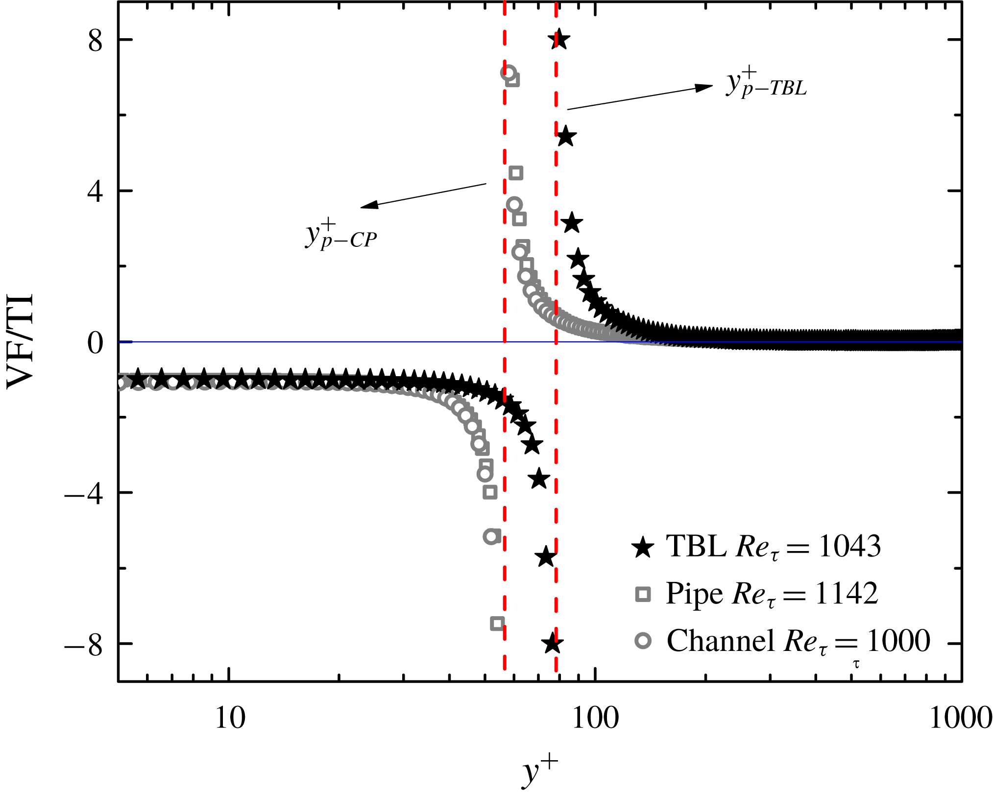
Figure 1. Ratio between the viscous shear force VF (
![]() $\unicode[STIX]{x2202}S^{+}/\unicode[STIX]{x2202}y^{+}$
) and turbulent inertial TI (
$\unicode[STIX]{x2202}S^{+}/\unicode[STIX]{x2202}y^{+}$
) and turbulent inertial TI (
![]() $\unicode[STIX]{x2202}W^{+}/\unicode[STIX]{x2202}y^{+}$
) showing the inner and outer flow regions demarcated by
$\unicode[STIX]{x2202}W^{+}/\unicode[STIX]{x2202}y^{+}$
) showing the inner and outer flow regions demarcated by
![]() $y^{+}=y_{p}^{+}$
where
$y^{+}=y_{p}^{+}$
where
![]() $\unicode[STIX]{x2202}W^{+}/\unicode[STIX]{x2202}y^{+}=0$
. Here,
$\unicode[STIX]{x2202}W^{+}/\unicode[STIX]{x2202}y^{+}=0$
. Here,
![]() $W^{+}=-\overline{u^{\prime }v^{\prime }}^{+}$
and
$W^{+}=-\overline{u^{\prime }v^{\prime }}^{+}$
and
![]() $S^{+}=\unicode[STIX]{x2202}U^{+}/\unicode[STIX]{x2202}y^{+}$
. Symbols are DNS data: stars from Schlatter et al. (Reference Schlatter, Li, Brethouwer, Johansson and Henningson2010); squares from Wu & Moin (Reference Wu and Moin2008); circles from Lee & Moser (Reference Lee and Moser2015).
$S^{+}=\unicode[STIX]{x2202}U^{+}/\unicode[STIX]{x2202}y^{+}$
. Symbols are DNS data: stars from Schlatter et al. (Reference Schlatter, Li, Brethouwer, Johansson and Henningson2010); squares from Wu & Moin (Reference Wu and Moin2008); circles from Lee & Moser (Reference Lee and Moser2015).
Recall the near-wall motion described by viscous units
![]() $y^{+}=yu_{\unicode[STIX]{x1D70F}}/\unicode[STIX]{x1D708}$
, and the outer inertial-dominated flow region by
$y^{+}=yu_{\unicode[STIX]{x1D70F}}/\unicode[STIX]{x1D708}$
, and the outer inertial-dominated flow region by
![]() $y/\unicode[STIX]{x1D6FF}$
. Sreenivasan (Reference Sreenivasan1988) proposed the
$y/\unicode[STIX]{x1D6FF}$
. Sreenivasan (Reference Sreenivasan1988) proposed the
![]() $Re_{\unicode[STIX]{x1D70F}}^{1/2}$
scaling of
$Re_{\unicode[STIX]{x1D70F}}^{1/2}$
scaling of
![]() $y_{p}^{+}$
for CP at high
$y_{p}^{+}$
for CP at high
![]() $Re_{\unicode[STIX]{x1D70F}}$
, validated by many others later (Klewicki Reference Klewicki2013; Chin et al.
Reference Chin, Philip, Klewicki, Ooi and Marusic2014; Lee & Moser Reference Lee and Moser2015; Ahn et al.
Reference Ahn, Lee and Sung2017). This can be derived as follows. Integrating (1.2) with respect to
$Re_{\unicode[STIX]{x1D70F}}$
, validated by many others later (Klewicki Reference Klewicki2013; Chin et al.
Reference Chin, Philip, Klewicki, Ooi and Marusic2014; Lee & Moser Reference Lee and Moser2015; Ahn et al.
Reference Ahn, Lee and Sung2017). This can be derived as follows. Integrating (1.2) with respect to
![]() $y^{+}$
yields
$y^{+}$
yields
(where the total stress
![]() $\unicode[STIX]{x1D70F}^{+}=1-y^{+}/Re_{\unicode[STIX]{x1D70F}}$
); further provided with the log law:
$\unicode[STIX]{x1D70F}^{+}=1-y^{+}/Re_{\unicode[STIX]{x1D70F}}$
); further provided with the log law:
it readily yields
by setting
![]() $\text{d}W^{+}/\text{d}y^{+}=0$
(
$\text{d}W^{+}/\text{d}y^{+}=0$
(
![]() $\unicode[STIX]{x1D705}$
is the von Kármán constant with its value taken around 0.45; see She et al. (Reference She, Chen and Hussain2017) and Chen et al. (Reference Chen, Hussain and She2018)). However, equation (2.3) is not accurate for CP at moderate
$\unicode[STIX]{x1D705}$
is the von Kármán constant with its value taken around 0.45; see She et al. (Reference She, Chen and Hussain2017) and Chen et al. (Reference Chen, Hussain and She2018)). However, equation (2.3) is not accurate for CP at moderate
![]() $Re_{\unicode[STIX]{x1D70F}}$
(Ahn et al.
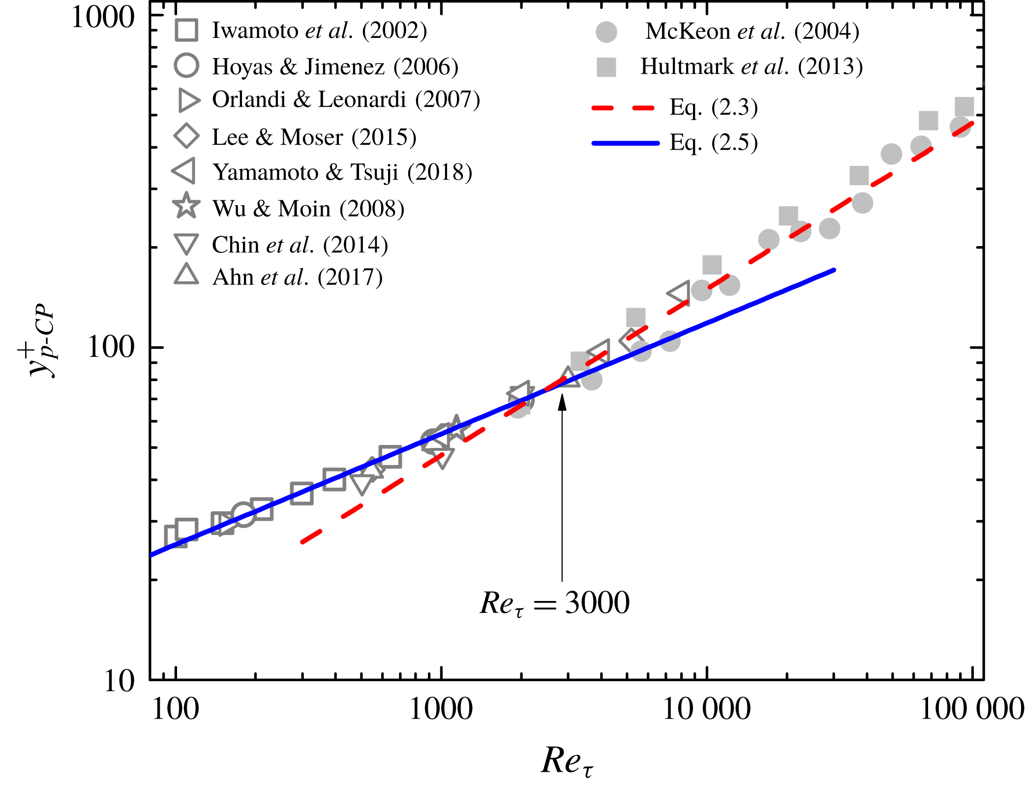
Reference Ahn, Lee and Sung2017), as seen in figure 2, showing a clear scaling transition.
$Re_{\unicode[STIX]{x1D70F}}$
(Ahn et al.
Reference Ahn, Lee and Sung2017), as seen in figure 2, showing a clear scaling transition.
This discrepancy of the classical scaling analysis is now well resolved here, through a specification of the buffer layer beneath the log layer, yielding a scaling transition towards lower
![]() $Re$
. Specifically, the viscous buffer layer extends from
$Re$
. Specifically, the viscous buffer layer extends from
![]() $y_{sub}^{+}\approx 9.7$
to
$y_{sub}^{+}\approx 9.7$
to
![]() $y_{buf}^{+}\approx 41$
, and we introduce a stress length (
$y_{buf}^{+}\approx 41$
, and we introduce a stress length (
![]() $\ell ^{+}=\sqrt{W^{+}}/S^{+}$
) which takes the following analytic form (She et al.
Reference She, Chen and Hussain2017; Chen et al.
Reference Chen, Hussain and She2018):
$\ell ^{+}=\sqrt{W^{+}}/S^{+}$
) which takes the following analytic form (She et al.
Reference She, Chen and Hussain2017; Chen et al.
Reference Chen, Hussain and She2018):
Substituting the approximation
![]() $S^{+}\approx 1/\ell ^{+}$
with (2.4c
) into (2.1), we obtain (2.3) for high
$S^{+}\approx 1/\ell ^{+}$
with (2.4c
) into (2.1), we obtain (2.3) for high
![]() $Re_{\unicode[STIX]{x1D70F}}$
; but for small
$Re_{\unicode[STIX]{x1D70F}}$
; but for small
![]() $Re_{\unicode[STIX]{x1D70F}}$
, with (2.4b
), we obtain:
$Re_{\unicode[STIX]{x1D70F}}$
, with (2.4b
), we obtain:
The existence of the buffer layer
![]() $y^{+2}$
scaling is the key to the present discovered scaling transition; this scaling arises from a local quasi-balance between the residue viscous effect
$y^{+2}$
scaling is the key to the present discovered scaling transition; this scaling arises from a local quasi-balance between the residue viscous effect
![]() $\unicode[STIX]{x1D700}$
and turbulent production
$\unicode[STIX]{x1D700}$
and turbulent production
![]() $SW$
, as follows. Introduce a shear eddy length:
$SW$
, as follows. Introduce a shear eddy length:
![]() $\ell _{\unicode[STIX]{x1D708}}=(W/S)^{3/4}\unicode[STIX]{x1D700}^{-1/4}$
; expansion analysis shows that
$\ell _{\unicode[STIX]{x1D708}}=(W/S)^{3/4}\unicode[STIX]{x1D700}^{-1/4}$
; expansion analysis shows that
![]() $\ell _{\unicode[STIX]{x1D708}}\propto y^{2}$
as
$\ell _{\unicode[STIX]{x1D708}}\propto y^{2}$
as
![]() $y\rightarrow 0$
(She et al.
Reference She, Chen and Hussain2017). Note that
$y\rightarrow 0$
(She et al.
Reference She, Chen and Hussain2017). Note that
![]() $\ell ^{+}=\ell _{\unicode[STIX]{x1D708}}^{+}\unicode[STIX]{x1D6E9}^{1/4}$
, where
$\ell ^{+}=\ell _{\unicode[STIX]{x1D708}}^{+}\unicode[STIX]{x1D6E9}^{1/4}$
, where
![]() $\unicode[STIX]{x1D6E9}=\unicode[STIX]{x1D700}/(SW)$
. As shown in She et al. (Reference She, Chen and Hussain2017), in the sublayer,
$\unicode[STIX]{x1D6E9}=\unicode[STIX]{x1D700}/(SW)$
. As shown in She et al. (Reference She, Chen and Hussain2017), in the sublayer,
![]() $\unicode[STIX]{x1D6E9}\ll 1$
and
$\unicode[STIX]{x1D6E9}\ll 1$
and
![]() $\ell _{\unicode[STIX]{x1D708}}^{+}\ll \ell ^{+}$
, and near-wall motion is dominated by random fluctuations; Taylor expansion results in (2.4a
). However, in the buffer layer,
$\ell _{\unicode[STIX]{x1D708}}^{+}\ll \ell ^{+}$
, and near-wall motion is dominated by random fluctuations; Taylor expansion results in (2.4a
). However, in the buffer layer,
![]() $\unicode[STIX]{x1D6E9}$
reaches a maximum of order unity (due to dominant effect of coherent motion); then,
$\unicode[STIX]{x1D6E9}$
reaches a maximum of order unity (due to dominant effect of coherent motion); then,
![]() $\ell ^{+}$
follows the scaling of
$\ell ^{+}$
follows the scaling of
![]() $\ell _{\unicode[STIX]{x1D708}}^{+}$
, which is (2.4b
). In the log layer where
$\ell _{\unicode[STIX]{x1D708}}^{+}$
, which is (2.4b
). In the log layer where
![]() $\unicode[STIX]{x1D6E9}\approx 1$
,
$\unicode[STIX]{x1D6E9}\approx 1$
,
![]() $\ell \approx \ell _{\unicode[STIX]{x1D708}}\propto y$
from homogeneous dilation symmetry (Chen et al.
Reference Chen, Hussain and She2018), which is (2.4c
).
$\ell \approx \ell _{\unicode[STIX]{x1D708}}\propto y$
from homogeneous dilation symmetry (Chen et al.
Reference Chen, Hussain and She2018), which is (2.4c
).
The realization of a buffer layer leads to a physical interpretation for the above scaling transition. Note that cascade is normally considered to result from the multiscale dynamics of turbulence (Frisch Reference Frisch1995). For the energy cascade, many studies have shown that it is caused by vortex stretching (for example, Goto Reference Goto and Eckhardt2009); for the momentum cascade, according to Jimenez (Reference Jimenez2012) and Yang & Lozano-Durán (Reference Yang and Lozano-Durán2017), it is carried out by a hierarchy of multiscale wall-attached eddies, which transfer momentum towards the wall until it is drained by the viscous effect. In Jimenez (Reference Jimenez2018), it is shown that the logarithmic eddies (or vortex clusters) scale as
![]() $y$
, which yield a scaling as predicted by (2.4c
); moreover, the buffer layer eddies are viewed as in an autonomous cycle having smaller sizes but with a higher Corrsin shear parameter, in accordance with (2.4b
), which indicates a smaller
$y$
, which yield a scaling as predicted by (2.4c
); moreover, the buffer layer eddies are viewed as in an autonomous cycle having smaller sizes but with a higher Corrsin shear parameter, in accordance with (2.4b
), which indicates a smaller
![]() $\ell$
and hence a larger
$\ell$
and hence a larger
![]() $S$
. Thus, approaching the wall from log to buffer layers, eddies with different spatial organizations, not surprisingly, would dictate different cascade processes.
$S$
. Thus, approaching the wall from log to buffer layers, eddies with different spatial organizations, not surprisingly, would dictate different cascade processes.
We now validate the predicted scaling transition by empirical data. Note that unlike for DNS data, it is quite inaccurate to determine
![]() $y_{p}^{+}$
from the experimentally measured
$y_{p}^{+}$
from the experimentally measured
![]() $\overline{u^{\prime }v^{\prime }}$
profile (for example, with large scatter); thus, an alternative way to determine
$\overline{u^{\prime }v^{\prime }}$
profile (for example, with large scatter); thus, an alternative way to determine
![]() $y_{p}^{+}$
is needed. Taking a
$y_{p}^{+}$
is needed. Taking a
![]() $y^{+}$
-derivative of (2.1) at
$y^{+}$
-derivative of (2.1) at
![]() $y^{+}=y_{p}^{+}$
yields
$y^{+}=y_{p}^{+}$
yields
which presents an equivalent way to find
![]() $y_{p}^{+}$
from
$y_{p}^{+}$
from
![]() $S^{+}(y^{+})=\unicode[STIX]{x2202}U^{+}/\unicode[STIX]{x2202}y^{+}$
. It is more accurate since the twice
$S^{+}(y^{+})=\unicode[STIX]{x2202}U^{+}/\unicode[STIX]{x2202}y^{+}$
. It is more accurate since the twice
![]() $y^{+}$
-derivative of
$y^{+}$
-derivative of
![]() $U^{+}(y^{+})$
can be obtained more reliably. For the Princeton SuperPipe (McKeon et al.
Reference McKeon, Li, Jiang, Morrison and Smits2004; Hultmark et al.
Reference Hultmark, Vallikivi, Bailey and Smits2013), as
$U^{+}(y^{+})$
can be obtained more reliably. For the Princeton SuperPipe (McKeon et al.
Reference McKeon, Li, Jiang, Morrison and Smits2004; Hultmark et al.
Reference Hultmark, Vallikivi, Bailey and Smits2013), as
![]() $\overline{u^{\prime }v^{\prime }}$
data are absent, Chin et al. (Reference Chin, Philip, Klewicki, Ooi and Marusic2014) and Ahn et al. (Reference Ahn, Lee and Sung2017) determine
$\overline{u^{\prime }v^{\prime }}$
data are absent, Chin et al. (Reference Chin, Philip, Klewicki, Ooi and Marusic2014) and Ahn et al. (Reference Ahn, Lee and Sung2017) determine
![]() $y_{p}^{+}$
in this way.
$y_{p}^{+}$
in this way.
Figure 2 shows that (2.5) agrees well with data at smaller
![]() $Re_{\unicode[STIX]{x1D70F}}$
, which, together with (2.3), indicates that the
$Re_{\unicode[STIX]{x1D70F}}$
, which, together with (2.3), indicates that the
![]() $Re_{\unicode[STIX]{x1D70F}}^{0.372}$
scaling by data fitting over the
$Re_{\unicode[STIX]{x1D70F}}^{0.372}$
scaling by data fitting over the
![]() $Re_{\unicode[STIX]{x1D70F}}$
range 500–5200 in Ahn et al. (Reference Ahn, Lee and Sung2017) is perhaps a misinterpretation. Furthermore, we predict that the scaling transition from
$Re_{\unicode[STIX]{x1D70F}}$
range 500–5200 in Ahn et al. (Reference Ahn, Lee and Sung2017) is perhaps a misinterpretation. Furthermore, we predict that the scaling transition from
![]() $Re_{\unicode[STIX]{x1D70F}}^{1/3}$
to
$Re_{\unicode[STIX]{x1D70F}}^{1/3}$
to
![]() $Re_{\unicode[STIX]{x1D70F}}^{1/2}$
takes place around
$Re_{\unicode[STIX]{x1D70F}}^{1/2}$
takes place around
![]() $Re_{\unicode[STIX]{x1D70F}}^{(crit)}=4\unicode[STIX]{x1D705}y_{buf}^{+2}\approx 3000$
for CP, by equating (2.5) with (2.3). Evidently, the
$Re_{\unicode[STIX]{x1D70F}}^{(crit)}=4\unicode[STIX]{x1D705}y_{buf}^{+2}\approx 3000$
for CP, by equating (2.5) with (2.3). Evidently, the
![]() $Re_{\unicode[STIX]{x1D70F}}^{1/3}$
scaling in figure 2 in turn supports the intermediate scaling (2.4b
) in the buffer layer. Whilst the scaling transition in CP has been shown in Chen et al. (Reference Chen, Hussain and She2018), here we include more data sets (for
$Re_{\unicode[STIX]{x1D70F}}^{1/3}$
scaling in figure 2 in turn supports the intermediate scaling (2.4b
) in the buffer layer. Whilst the scaling transition in CP has been shown in Chen et al. (Reference Chen, Hussain and She2018), here we include more data sets (for
![]() $Re_{\unicode[STIX]{x1D70F}}$
covering three decades) to provide compelling evidence of scaling transition. More importantly, the theme of the current paper is to reveal and demonstrate, under the same analysis, the non-universal scaling transition among CP (internal) and TBL (external) flows, as we discuss below.
$Re_{\unicode[STIX]{x1D70F}}$
covering three decades) to provide compelling evidence of scaling transition. More importantly, the theme of the current paper is to reveal and demonstrate, under the same analysis, the non-universal scaling transition among CP (internal) and TBL (external) flows, as we discuss below.
Applying the above analysis to TBL, a new element arises – that is, a small but finite mean wall-normal velocity
![]() $V$
. The small
$V$
. The small
![]() $V$
changes the
$V$
changes the
![]() $U$
profile only slightly, but leads to its non-trivial streamwise development, and a different total stress, i.e.
$U$
profile only slightly, but leads to its non-trivial streamwise development, and a different total stress, i.e.
![]() $\unicode[STIX]{x1D70F}^{+}=1-\int _{0}^{y^{+}}(U^{+}(\unicode[STIX]{x2202}V^{+}/\unicode[STIX]{x2202}y^{\prime })-V^{+}(\unicode[STIX]{x2202}U^{+}/\unicode[STIX]{x2202}y^{\prime }))\,\text{d}y^{\prime }$
. For determining
$\unicode[STIX]{x1D70F}^{+}=1-\int _{0}^{y^{+}}(U^{+}(\unicode[STIX]{x2202}V^{+}/\unicode[STIX]{x2202}y^{\prime })-V^{+}(\unicode[STIX]{x2202}U^{+}/\unicode[STIX]{x2202}y^{\prime }))\,\text{d}y^{\prime }$
. For determining
![]() $V$
, we consider the mean kinetic energy equation of
$V$
, we consider the mean kinetic energy equation of
![]() $V$
, in which the dissipation term (that is,
$V$
, in which the dissipation term (that is,
![]() $\unicode[STIX]{x1D716}_{V}=\unicode[STIX]{x1D708}(\unicode[STIX]{x2202}V/\unicode[STIX]{x2202}y)^{2}$
) can be specified by a dimensional analysis using
$\unicode[STIX]{x1D716}_{V}=\unicode[STIX]{x1D708}(\unicode[STIX]{x2202}V/\unicode[STIX]{x2202}y)^{2}$
) can be specified by a dimensional analysis using
![]() $\unicode[STIX]{x1D708}$
,
$\unicode[STIX]{x1D708}$
,
![]() $\unicode[STIX]{x1D6FF}$
and free-stream wall-normal velocity
$\unicode[STIX]{x1D6FF}$
and free-stream wall-normal velocity
![]() $V_{e}$
, yielding
$V_{e}$
, yielding
![]() $\unicode[STIX]{x1D716}_{V}=(\unicode[STIX]{x1D708}V_{e}^{2}/\unicode[STIX]{x1D6FF}^{2})\unicode[STIX]{x1D6FA}(y/\unicode[STIX]{x1D6FF})$
. The self-similar function
$\unicode[STIX]{x1D716}_{V}=(\unicode[STIX]{x1D708}V_{e}^{2}/\unicode[STIX]{x1D6FF}^{2})\unicode[STIX]{x1D6FA}(y/\unicode[STIX]{x1D6FF})$
. The self-similar function
![]() $\unicode[STIX]{x1D6FA}$
satisfies
$\unicode[STIX]{x1D6FA}$
satisfies
![]() $\unicode[STIX]{x1D6FA}(0)=0$
, which suggests a simple linear approximation:
$\unicode[STIX]{x1D6FA}(0)=0$
, which suggests a simple linear approximation:
![]() $\unicode[STIX]{x1D6FA}=\unicode[STIX]{x1D714}_{1}y/\unicode[STIX]{x1D6FF}$
, and then,
$\unicode[STIX]{x1D6FA}=\unicode[STIX]{x1D714}_{1}y/\unicode[STIX]{x1D6FF}$
, and then,
![]() $\unicode[STIX]{x1D716}_{V}=\unicode[STIX]{x1D714}_{1}(\unicode[STIX]{x1D708}V_{e}^{2}/\unicode[STIX]{x1D6FF}^{2})(y/\unicode[STIX]{x1D6FF})$
. Using the definition of
$\unicode[STIX]{x1D716}_{V}=\unicode[STIX]{x1D714}_{1}(\unicode[STIX]{x1D708}V_{e}^{2}/\unicode[STIX]{x1D6FF}^{2})(y/\unicode[STIX]{x1D6FF})$
. Using the definition of
![]() $\unicode[STIX]{x1D716}_{V}$
and integrating it with respect to
$\unicode[STIX]{x1D716}_{V}$
and integrating it with respect to
![]() $y$
, one obtains
$y$
, one obtains
where
![]() $\unicode[STIX]{x1D714}_{1}=(3/2)^{2}=9/4$
due to
$\unicode[STIX]{x1D714}_{1}=(3/2)^{2}=9/4$
due to
![]() $V(0)=0$
and
$V(0)=0$
and
![]() $V(\unicode[STIX]{x1D6FF})=V_{e}$
. Figure 3 shows that (2.7) agrees closely with DNS data, which thus well describes the data collapse found by Wei & Klewicki (Reference Wei and Klewicki2016).
$V(\unicode[STIX]{x1D6FF})=V_{e}$
. Figure 3 shows that (2.7) agrees closely with DNS data, which thus well describes the data collapse found by Wei & Klewicki (Reference Wei and Klewicki2016).
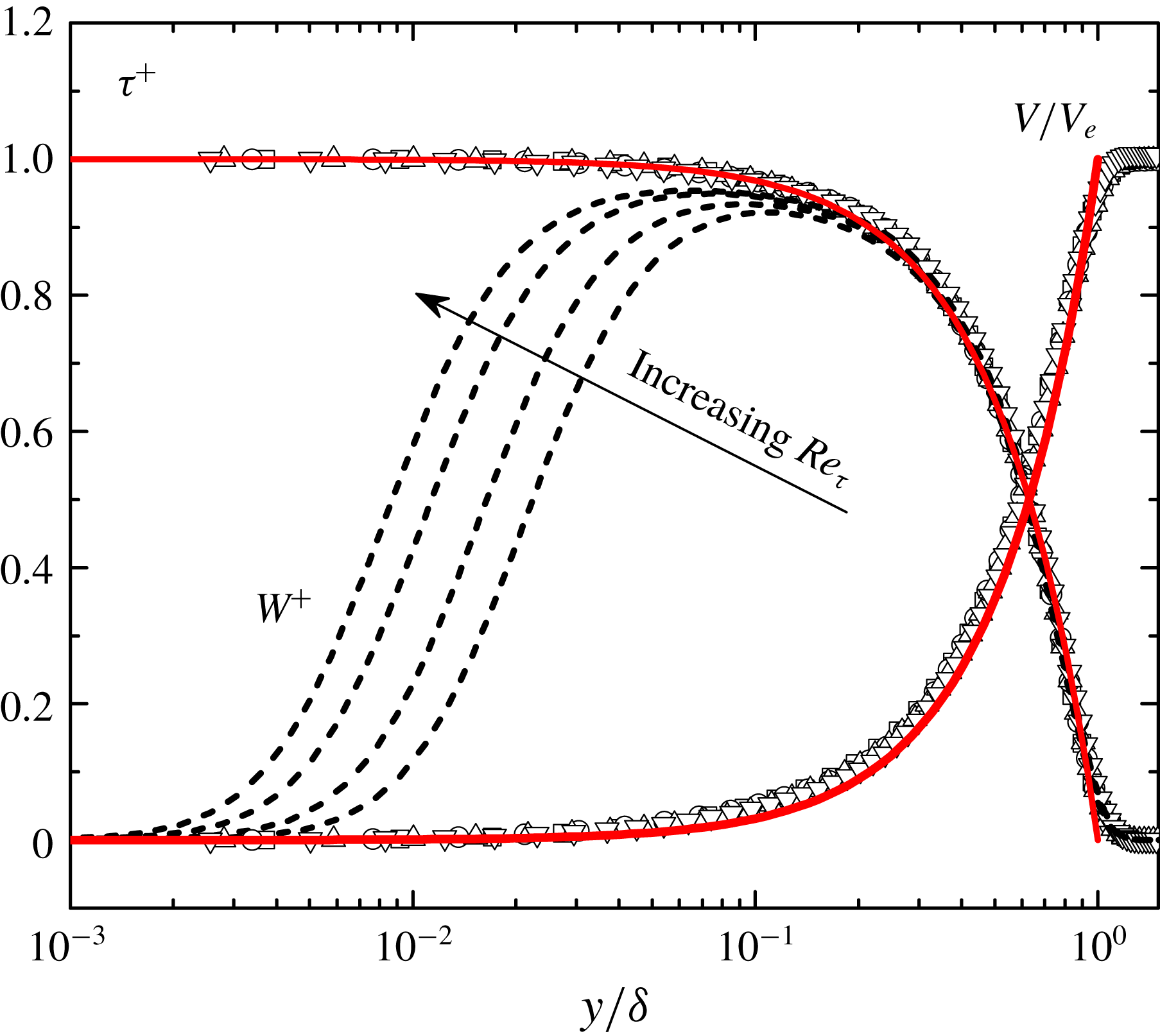
Figure 3. DNS profiles (Schlatter et al.
Reference Schlatter, Li, Brethouwer, Johansson and Henningson2010) of total stress
![]() $\unicode[STIX]{x1D70F}^{+}$
(symbols), mean wall-normal velocity
$\unicode[STIX]{x1D70F}^{+}$
(symbols), mean wall-normal velocity
![]() $V/V_{e}$
(symbols) and mean momentum flux (Reynolds shear stress)
$V/V_{e}$
(symbols) and mean momentum flux (Reynolds shear stress)
![]() $W^{+}=-\overline{u^{\prime }v^{\prime }}^{+}$
(dashed lines) in TBL. Profiles of
$W^{+}=-\overline{u^{\prime }v^{\prime }}^{+}$
(dashed lines) in TBL. Profiles of
![]() $\unicode[STIX]{x1D70F}^{+}$
and
$\unicode[STIX]{x1D70F}^{+}$
and
![]() $V/V_{e}$
at four different cases
$V/V_{e}$
at four different cases
![]() $Re_{\unicode[STIX]{x1D70F}}=492$
, 671, 974 and 1271 collapse. Solid lines indicate our theories: equation (2.7) for
$Re_{\unicode[STIX]{x1D70F}}=492$
, 671, 974 and 1271 collapse. Solid lines indicate our theories: equation (2.7) for
![]() $V$
and (2.8) for
$V$
and (2.8) for
![]() $\unicode[STIX]{x1D70F}^{+}$
.
$\unicode[STIX]{x1D70F}^{+}$
.
Based on (2.7),
![]() $\unicode[STIX]{x1D70F}^{+}$
in TBL is obtained:
$\unicode[STIX]{x1D70F}^{+}$
in TBL is obtained:
To see this, we first denote
![]() $U^{+}\propto (y^{+})^{\unicode[STIX]{x1D709}}$
, where according to the log law (2.2),
$U^{+}\propto (y^{+})^{\unicode[STIX]{x1D709}}$
, where according to the log law (2.2),
![]() $\unicode[STIX]{x1D709}-1\approx -1$
or
$\unicode[STIX]{x1D709}-1\approx -1$
or
![]() $\unicode[STIX]{x1D709}\approx 0$
(also see Barenblatt (Reference Barenblatt1993), where
$\unicode[STIX]{x1D709}\approx 0$
(also see Barenblatt (Reference Barenblatt1993), where
![]() $\unicode[STIX]{x1D709}\propto 1/\ln Re$
). Then, substituting
$\unicode[STIX]{x1D709}\propto 1/\ln Re$
). Then, substituting
![]() $U^{+}\propto (y^{+})^{\unicode[STIX]{x1D709}}$
and
$U^{+}\propto (y^{+})^{\unicode[STIX]{x1D709}}$
and
![]() $V^{+}\propto (y^{+})^{3/2}$
of (2.7) into
$V^{+}\propto (y^{+})^{3/2}$
of (2.7) into
![]() $\unicode[STIX]{x1D70F}^{+}=1-\int _{0}^{y^{+}}(U^{+}(\unicode[STIX]{x2202}V^{+}/\unicode[STIX]{x2202}y^{\prime })-V^{+}(\unicode[STIX]{x2202}U^{+}/\unicode[STIX]{x2202}y^{\prime }))\,\text{d}y^{\prime }$
yields
$\unicode[STIX]{x1D70F}^{+}=1-\int _{0}^{y^{+}}(U^{+}(\unicode[STIX]{x2202}V^{+}/\unicode[STIX]{x2202}y^{\prime })-V^{+}(\unicode[STIX]{x2202}U^{+}/\unicode[STIX]{x2202}y^{\prime }))\,\text{d}y^{\prime }$
yields
![]() $1-\unicode[STIX]{x1D70F}^{+}\propto (y^{+})^{3/2+\unicode[STIX]{x1D709}}$
. As
$1-\unicode[STIX]{x1D70F}^{+}\propto (y^{+})^{3/2+\unicode[STIX]{x1D709}}$
. As
![]() $\unicode[STIX]{x1D709}\approx 0$
,
$\unicode[STIX]{x1D709}\approx 0$
,
![]() $1-\unicode[STIX]{x1D70F}^{+}\approx \unicode[STIX]{x1D70F}_{0}y^{+3/2}$
. Moreover, as
$1-\unicode[STIX]{x1D70F}^{+}\approx \unicode[STIX]{x1D70F}_{0}y^{+3/2}$
. Moreover, as
![]() $\unicode[STIX]{x1D70F}^{+}=0$
at
$\unicode[STIX]{x1D70F}^{+}=0$
at
![]() $y^{+}=\unicode[STIX]{x1D6FF}^{+}$
(or
$y^{+}=\unicode[STIX]{x1D6FF}^{+}$
(or
![]() $y^{+}=Re_{\unicode[STIX]{x1D70F}}$
),
$y^{+}=Re_{\unicode[STIX]{x1D70F}}$
),
![]() $\unicode[STIX]{x1D70F}_{0}=Re_{\unicode[STIX]{x1D70F}}^{-3/2}$
, and thus (2.8). Compared to
$\unicode[STIX]{x1D70F}_{0}=Re_{\unicode[STIX]{x1D70F}}^{-3/2}$
, and thus (2.8). Compared to
![]() $1-\unicode[STIX]{x1D70F}^{+}=y^{+}/Re_{\unicode[STIX]{x1D70F}}$
in CP,
$1-\unicode[STIX]{x1D70F}^{+}=y^{+}/Re_{\unicode[STIX]{x1D70F}}$
in CP,
![]() $1-\unicode[STIX]{x1D70F}^{+}$
in TBL is higher at the same
$1-\unicode[STIX]{x1D70F}^{+}$
in TBL is higher at the same
![]() $y$
location due to
$y$
location due to
![]() $V$
. This explains earlier observations in Degraaff & Eaton (Reference Degraaff and Eaton2000), well supported by DNS data in figure 3.
$V$
. This explains earlier observations in Degraaff & Eaton (Reference Degraaff and Eaton2000), well supported by DNS data in figure 3.
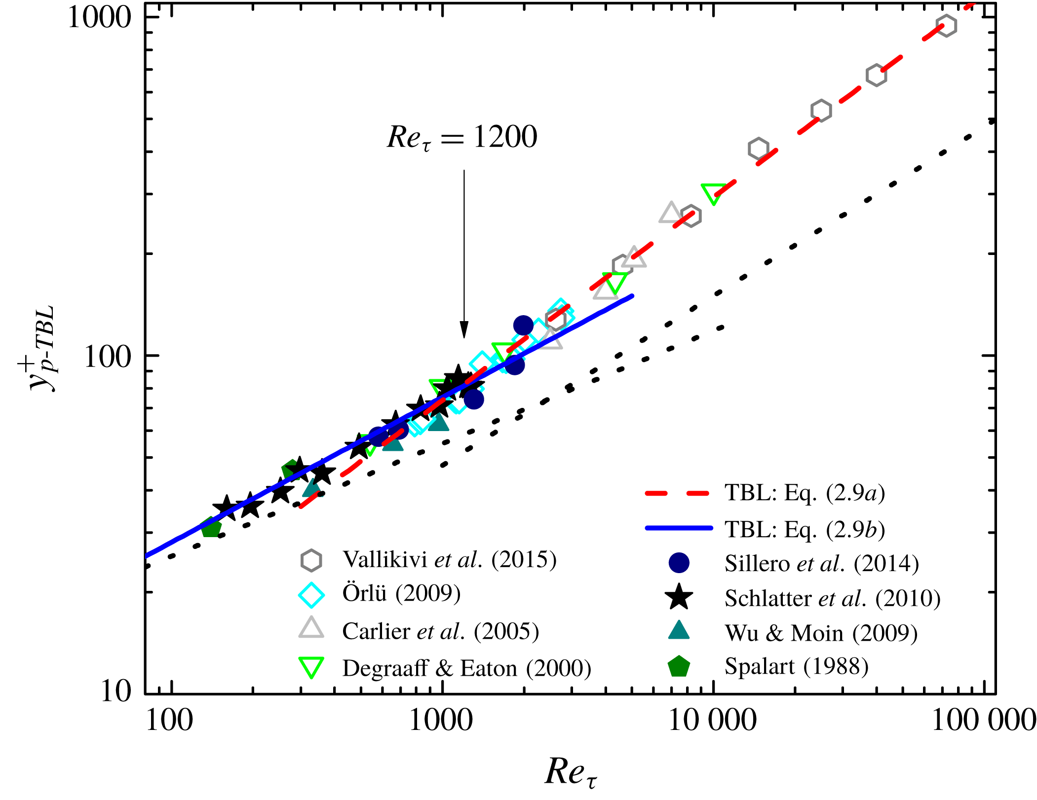
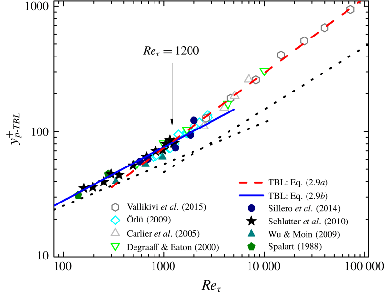
Figure 4. The same plot as figure 2 but for TBL. Solid symbols, DNS; open symbols, experiments. Note that the open symbols of experiments are measured by using (2.10) – agreeing well with solid symbols of DNS data in the overlapped
![]() $Re_{\unicode[STIX]{x1D70F}}$
range (from 500 to 2000). For comparison, two dotted lines for CP are included, which show much smaller
$Re_{\unicode[STIX]{x1D70F}}$
range (from 500 to 2000). For comparison, two dotted lines for CP are included, which show much smaller
![]() $y_{p}^{+}$
for high
$y_{p}^{+}$
for high
![]() $Re$
.
$Re$
.
Completing the previous analysis of
![]() $y_{p}^{+}$
using (2.8) yields
$y_{p}^{+}$
using (2.8) yields
for large
![]() $Re_{\unicode[STIX]{x1D70F}}$
, and
$Re_{\unicode[STIX]{x1D70F}}$
, and
for small
![]() $Re_{\unicode[STIX]{x1D70F}}$
. The relation defining
$Re_{\unicode[STIX]{x1D70F}}$
. The relation defining
![]() $y_{p}^{+}$
from
$y_{p}^{+}$
from
![]() $\text{d}S^{+}/\text{d}y^{+}$
for TBL takes the following form:
$\text{d}S^{+}/\text{d}y^{+}$
for TBL takes the following form:
in sharp contrast to (2.6) for CP. Again, equating (2.9b
) and (2.9a
), the scaling transition occurs around
![]() $Re_{\unicode[STIX]{x1D70F}}=2(9\unicode[STIX]{x1D705}^{2}y_{buf}^{+5})^{1/3}\approx 1200$
.
$Re_{\unicode[STIX]{x1D70F}}=2(9\unicode[STIX]{x1D705}^{2}y_{buf}^{+5})^{1/3}\approx 1200$
.
Figure 4 shows the good agreement between the prediction (2.9) and data. Note that
![]() $y_{p-TBL}^{+}$
between DNS data (Spalart Reference Spalart1988; Wu & Moin Reference Wu and Moin2009; Sillero, Jimnez & Moser Reference Sillero, Jimnez and Moser2014) – by pinpointing the maximum of the
$y_{p-TBL}^{+}$
between DNS data (Spalart Reference Spalart1988; Wu & Moin Reference Wu and Moin2009; Sillero, Jimnez & Moser Reference Sillero, Jimnez and Moser2014) – by pinpointing the maximum of the
![]() $W^{+}$
profile directly – and experimental data (Degraaff & Eaton Reference Degraaff and Eaton2000; Carlier & Stanislas Reference Carlier and Stanislas2005; Örlü Reference Örlü2009; Vallikivi, Ganapathisubramani & Smits Reference Vallikivi, Ganapathisubramani and Smits2015) – by using (2.10) – agree well with each other in the overlapped
$W^{+}$
profile directly – and experimental data (Degraaff & Eaton Reference Degraaff and Eaton2000; Carlier & Stanislas Reference Carlier and Stanislas2005; Örlü Reference Örlü2009; Vallikivi, Ganapathisubramani & Smits Reference Vallikivi, Ganapathisubramani and Smits2015) – by using (2.10) – agree well with each other in the overlapped
![]() $Re_{\unicode[STIX]{x1D70F}}$
range, hence supporting the validity of (2.10). Moreover, we have checked that
$Re_{\unicode[STIX]{x1D70F}}$
range, hence supporting the validity of (2.10). Moreover, we have checked that
![]() $W^{+}\approx 1-(y^{+}/Re_{\unicode[STIX]{x1D70F}})^{3/2}$
agrees closely with the available high-
$W^{+}\approx 1-(y^{+}/Re_{\unicode[STIX]{x1D70F}})^{3/2}$
agrees closely with the available high-
![]() $Re_{\unicode[STIX]{x1D70F}}$
experimental
$Re_{\unicode[STIX]{x1D70F}}$
experimental
![]() $W^{+}$
profile in the outer flow region; thus (2.8) and hence (2.10) seem robust. Incidentally, a
$W^{+}$
profile in the outer flow region; thus (2.8) and hence (2.10) seem robust. Incidentally, a
![]() $Re_{\unicode[STIX]{x1D703}}^{0.63}$
scaling was reported for TBL based on fitting of experimental data (Fernholz & Finleyt Reference Fernholz and Finleyt1996), which is quite close to our (2.9a
) (as
$Re_{\unicode[STIX]{x1D703}}^{0.63}$
scaling was reported for TBL based on fitting of experimental data (Fernholz & Finleyt Reference Fernholz and Finleyt1996), which is quite close to our (2.9a
) (as
![]() $Re_{\unicode[STIX]{x1D703}}/Re_{\unicode[STIX]{x1D70F}}\sim O(1)$
; see Chen & She (Reference Chen and She2016), Monkewitz, Chauhan & Nagib (Reference Monkewitz, Chauhan and Nagib2007)). However, those TBL experimental data have too much scatter, and hence are not included here.
$Re_{\unicode[STIX]{x1D703}}/Re_{\unicode[STIX]{x1D70F}}\sim O(1)$
; see Chen & She (Reference Chen and She2016), Monkewitz, Chauhan & Nagib (Reference Monkewitz, Chauhan and Nagib2007)). However, those TBL experimental data have too much scatter, and hence are not included here.
The non-universal scaling transition is also reflected in the maximum momentum flux
![]() $W_{p}^{+}(=-\overline{u^{\prime }v^{\prime }}_{p}^{+})$
, which is obtained by substituting
$W_{p}^{+}(=-\overline{u^{\prime }v^{\prime }}_{p}^{+})$
, which is obtained by substituting
![]() $y_{p}^{+}$
in (2.1). For large
$y_{p}^{+}$
in (2.1). For large
![]() $Re_{\unicode[STIX]{x1D70F}}$
, using (2.9a
) for TBL and (2.3) for CP, respectively, we have
$Re_{\unicode[STIX]{x1D70F}}$
, using (2.9a
) for TBL and (2.3) for CP, respectively, we have
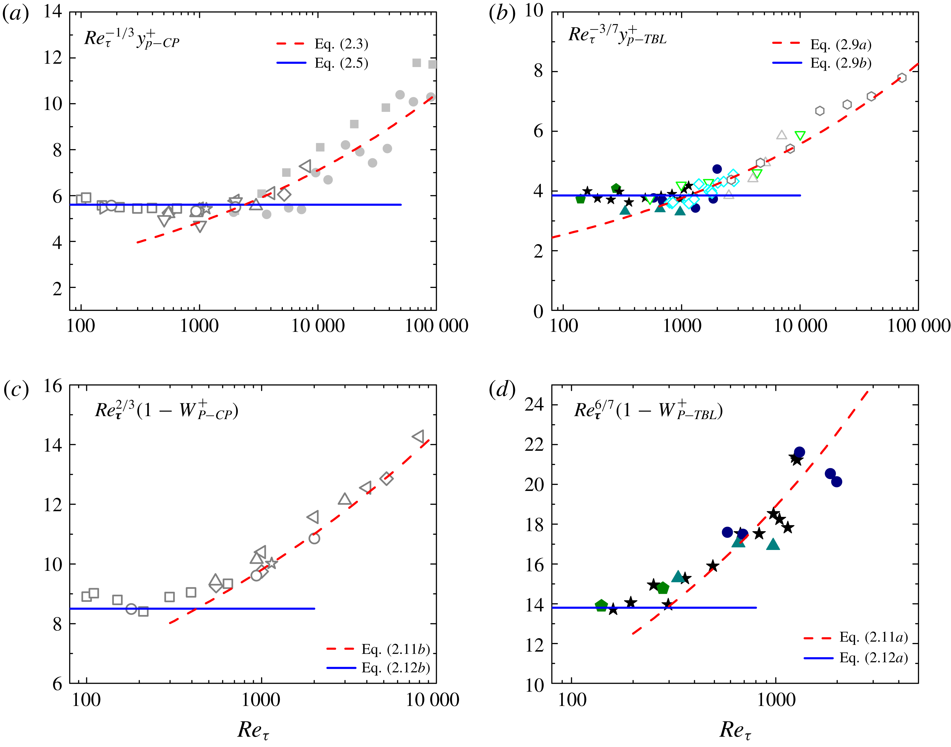
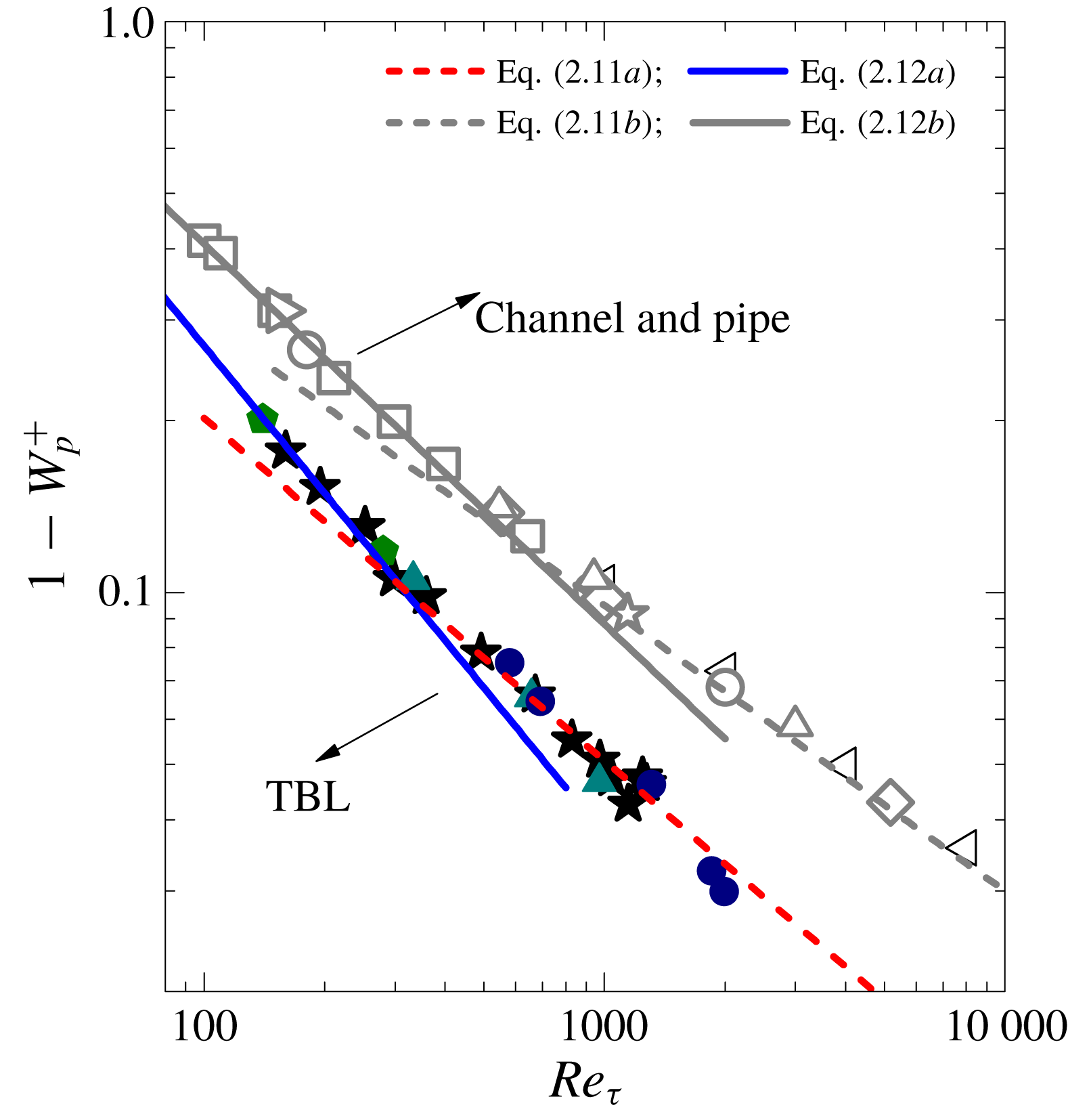
Figure 6. Compensated plots of
![]() $y_{p}^{+}$
scaling for channel and pipe flows (a), and for TBL flows (b). Compensated plots of
$y_{p}^{+}$
scaling for channel and pipe flows (a), and for TBL flows (b). Compensated plots of
![]() $1-W_{p}^{+}$
scaling for channel and pipe flows (c), and for TBL flows (d). Lines are scaling predictions; symbols are data – the same as in figure 2 (for channel and pipe) and figure 4 (for TBL).
$1-W_{p}^{+}$
scaling for channel and pipe flows (c), and for TBL flows (d). Lines are scaling predictions; symbols are data – the same as in figure 2 (for channel and pipe) and figure 4 (for TBL).
To better display the scaling transition, we show in figure 6 the compensated plots of both
![]() $y_{p}^{+}$
and
$y_{p}^{+}$
and
![]() $1-W_{p}^{+}$
. The plateaus in figure 6(a,b) justify the small-
$1-W_{p}^{+}$
. The plateaus in figure 6(a,b) justify the small-
![]() $Re$
scaling
$Re$
scaling
![]() $Re_{\unicode[STIX]{x1D70F}}^{1/3}$
for CP and
$Re_{\unicode[STIX]{x1D70F}}^{1/3}$
for CP and
![]() $Re_{\unicode[STIX]{x1D70F}}^{3/7}$
for TBL, respectively; data departing from the plateaus indicate the scaling transition with increasing
$Re_{\unicode[STIX]{x1D70F}}^{3/7}$
for TBL, respectively; data departing from the plateaus indicate the scaling transition with increasing
![]() $Re_{\unicode[STIX]{x1D70F}}$
. For example, for channel flows, most DNS data follow the
$Re_{\unicode[STIX]{x1D70F}}$
. For example, for channel flows, most DNS data follow the
![]() $Re_{\unicode[STIX]{x1D70F}}^{1/3}$
scaling; however, DNS data at
$Re_{\unicode[STIX]{x1D70F}}^{1/3}$
scaling; however, DNS data at
![]() $Re_{\unicode[STIX]{x1D70F}}=4000$
(Yamamoto & Tsuji Reference Yamamoto and Tsuji2018), 5200 (Lee & Moser Reference Lee and Moser2015) and 8000 (Yamamoto & Tsuji Reference Yamamoto and Tsuji2018) agree better with (2.3) than with (2.5), hence clearly displaying the predicted scaling transition. Moreover, figure 6(c,d) show the transition in
$Re_{\unicode[STIX]{x1D70F}}=4000$
(Yamamoto & Tsuji Reference Yamamoto and Tsuji2018), 5200 (Lee & Moser Reference Lee and Moser2015) and 8000 (Yamamoto & Tsuji Reference Yamamoto and Tsuji2018) agree better with (2.3) than with (2.5), hence clearly displaying the predicted scaling transition. Moreover, figure 6(c,d) show the transition in
![]() $1-W_{p}^{+}$
, where most DNS data are in the large-scaling regimes. It is unknown why the scaling transition for
$1-W_{p}^{+}$
, where most DNS data are in the large-scaling regimes. It is unknown why the scaling transition for
![]() $1-W_{p}^{+}$
is less sharp and occurs earlier than that for
$1-W_{p}^{+}$
is less sharp and occurs earlier than that for
![]() $y_{p}^{+}$
, possibly due to
$y_{p}^{+}$
, possibly due to
![]() $1-W_{p}^{+}$
being a subleading-order behaviour of the momentum cascade (the leading-order behaviour is
$1-W_{p}^{+}$
being a subleading-order behaviour of the momentum cascade (the leading-order behaviour is
![]() $W^{+}\approx 1$
as
$W^{+}\approx 1$
as
![]() $Re\rightarrow \infty$
), which varies mildly but sensitively with increasing
$Re\rightarrow \infty$
), which varies mildly but sensitively with increasing
![]() $Re$
. A further examination on the vorticity transport of
$Re$
. A further examination on the vorticity transport of
![]() $W^{+}$
(Chin et al.
Reference Chin, Philip, Klewicki, Ooi and Marusic2014) is perhaps helpful to answer this question. Note the deviation from (2.11a
) for the two largest
$W^{+}$
(Chin et al.
Reference Chin, Philip, Klewicki, Ooi and Marusic2014) is perhaps helpful to answer this question. Note the deviation from (2.11a
) for the two largest
![]() $Re$
data points in figure 6(d), which may suggest a new scaling trend but may also be caused by insufficiently large simulation domains – an issue to clarify when high-quality data at large
$Re$
data points in figure 6(d), which may suggest a new scaling trend but may also be caused by insufficiently large simulation domains – an issue to clarify when high-quality data at large
![]() $Re$
are available.
$Re$
are available.
According to the DNS data trend and our predictions in figure 5,
![]() $1-W_{p}^{+}<0.03$
for CP at
$1-W_{p}^{+}<0.03$
for CP at
![]() $Re_{\unicode[STIX]{x1D70F}}=10^{4}$
and
$Re_{\unicode[STIX]{x1D70F}}=10^{4}$
and
![]() $1-W_{p}^{+}<0.01$
at
$1-W_{p}^{+}<0.01$
at
![]() $Re_{\unicode[STIX]{x1D70F}}=10^{5}$
; the deviation from unity is even smaller for TBL (i.e.
$Re_{\unicode[STIX]{x1D70F}}=10^{5}$
; the deviation from unity is even smaller for TBL (i.e.
![]() $1-W_{p}^{+}<0.01$
at
$1-W_{p}^{+}<0.01$
at
![]() $Re_{\unicode[STIX]{x1D70F}}=10^{4}$
and
$Re_{\unicode[STIX]{x1D70F}}=10^{4}$
and
![]() $1-W_{p}^{+}<0.003$
at
$1-W_{p}^{+}<0.003$
at
![]() $Re_{\unicode[STIX]{x1D70F}}=10^{5}$
). These small deviations are far beyond the experimental resolutions, and hence we use DNS data to validate our predictions of
$Re_{\unicode[STIX]{x1D70F}}=10^{5}$
). These small deviations are far beyond the experimental resolutions, and hence we use DNS data to validate our predictions of
![]() $1-W_{p}^{+}$
. It is clear from figures 5 and 6(c,d) that the predicted large-
$1-W_{p}^{+}$
. It is clear from figures 5 and 6(c,d) that the predicted large-
![]() $Re$
scalings are well supported by both CP and TBL DNS data; while for small
$Re$
scalings are well supported by both CP and TBL DNS data; while for small
![]() $Re$
, there are only a few data points in these figures, showing mild deviations from our large-
$Re$
, there are only a few data points in these figures, showing mild deviations from our large-
![]() $Re$
predictions, but they all follow closely our scaling predictions for small
$Re$
predictions, but they all follow closely our scaling predictions for small
![]() $Re$
. One can of course fit the solid symbols in figure 5 (i.e.
$Re$
. One can of course fit the solid symbols in figure 5 (i.e.
![]() $1-W_{p}^{+}$
of TBL) by a single power law (for example,
$1-W_{p}^{+}$
of TBL) by a single power law (for example,
![]() $6.2Re_{\unicode[STIX]{x1D70F}}^{-0.7}$
), but then one cannot explain these fitting parameters. Moreover, the fitting may be another data misinterpretation, as there is a scaling transition according to our theory.
$6.2Re_{\unicode[STIX]{x1D70F}}^{-0.7}$
), but then one cannot explain these fitting parameters. Moreover, the fitting may be another data misinterpretation, as there is a scaling transition according to our theory.
Finally, let us envisage the existence of an asymptotic flow state for CP and TBL by the probable full coupling between energy and momentum cascades. While the energy cascade is more developed in the bulk flow region (
![]() $y^{+}>y_{Q}^{+}$
with
$y^{+}>y_{Q}^{+}$
with
![]() $y_{Q}^{+}\sim 150{-}200$
) where production quasi-balances dissipation, the momentum cascade is centred at
$y_{Q}^{+}\sim 150{-}200$
) where production quasi-balances dissipation, the momentum cascade is centred at
![]() $y^{+}=y_{p}^{+}$
, which is smaller than
$y^{+}=y_{p}^{+}$
, which is smaller than
![]() $y_{Q}^{+}$
at moderate
$y_{Q}^{+}$
at moderate
![]() $Re_{\unicode[STIX]{x1D70F}}$
but would overtake
$Re_{\unicode[STIX]{x1D70F}}$
but would overtake
![]() $y_{Q}^{+}$
as
$y_{Q}^{+}$
as
![]() $Re_{\unicode[STIX]{x1D70F}}$
increases. Therefore, equating
$Re_{\unicode[STIX]{x1D70F}}$
increases. Therefore, equating
![]() $y_{p}^{+}=y_{Q}^{+}$
, we obtain a critical
$y_{p}^{+}=y_{Q}^{+}$
, we obtain a critical
![]() $Re_{\unicode[STIX]{x1D70F}}$
indicating the onset of co-existence of two cascades in the bulk flow. It was speculated (Chen et al.
Reference Chen, Wei, Hussain and She2015) that at this state the energy cascade will be modified, leading to anomalous energy dissipation. Taking
$Re_{\unicode[STIX]{x1D70F}}$
indicating the onset of co-existence of two cascades in the bulk flow. It was speculated (Chen et al.
Reference Chen, Wei, Hussain and She2015) that at this state the energy cascade will be modified, leading to anomalous energy dissipation. Taking
![]() $y_{Q}^{+}\approx 150$
for CP (Vincenti et al.
Reference Vincenti, Klewicki, Morrill-Winter, White and Wosnik2013) yields
$y_{Q}^{+}\approx 150$
for CP (Vincenti et al.
Reference Vincenti, Klewicki, Morrill-Winter, White and Wosnik2013) yields
![]() $Re_{\unicode[STIX]{x1D70F}}^{(c)}=\unicode[STIX]{x1D705}y_{Q}^{+2}\approx 10\,100$
, which interestingly matches
$Re_{\unicode[STIX]{x1D70F}}^{(c)}=\unicode[STIX]{x1D705}y_{Q}^{+2}\approx 10\,100$
, which interestingly matches
![]() $Re_{\unicode[STIX]{x1D70F}}\approx 10\,481$
for the emergence of an outer
$Re_{\unicode[STIX]{x1D70F}}\approx 10\,481$
for the emergence of an outer
![]() $\overline{u^{\prime }u^{\prime }}$
peak in the Princeton SuperPipe (Hultmark et al.
Reference Hultmark, Vallikivi, Bailey and Smits2013). For TBL,
$\overline{u^{\prime }u^{\prime }}$
peak in the Princeton SuperPipe (Hultmark et al.
Reference Hultmark, Vallikivi, Bailey and Smits2013). For TBL,
![]() $y_{Q}^{+}\approx 200$
(Schlatter et al.
Reference Schlatter, Li, Brethouwer, Johansson and Henningson2010), using
$y_{Q}^{+}\approx 200$
(Schlatter et al.
Reference Schlatter, Li, Brethouwer, Johansson and Henningson2010), using
![]() $y_{p}^{+}$
in (2.9) we obtain another critical
$y_{p}^{+}$
in (2.9) we obtain another critical
![]() $Re_{\unicode[STIX]{x1D70F}}^{(c)}\approx 5500$
, very close to
$Re_{\unicode[STIX]{x1D70F}}^{(c)}\approx 5500$
, very close to
![]() $Re_{\unicode[STIX]{x1D70F}}\approx 6400$
where the outer
$Re_{\unicode[STIX]{x1D70F}}\approx 6400$
where the outer
![]() $\overline{u^{\prime }u^{\prime }}$
peak in TBL is observed (Vincenti et al.
Reference Vincenti, Klewicki, Morrill-Winter, White and Wosnik2013). This apparent link to the emergence of the
$\overline{u^{\prime }u^{\prime }}$
peak in TBL is observed (Vincenti et al.
Reference Vincenti, Klewicki, Morrill-Winter, White and Wosnik2013). This apparent link to the emergence of the
![]() $\overline{u^{\prime }u^{\prime }}$
outer peak is intriguing, which implies a possible asymptotic flow regime for Reynolds number larger than
$\overline{u^{\prime }u^{\prime }}$
outer peak is intriguing, which implies a possible asymptotic flow regime for Reynolds number larger than
![]() $Re_{\unicode[STIX]{x1D70F}}^{(c)}$
.
$Re_{\unicode[STIX]{x1D70F}}^{(c)}$
.
3 Conclusion
In this paper, we establish a non-universal
![]() $Re$
-scaling transition for both the peak location and the magnitude of Reynolds shear stress (momentum cascade). Particularly, at large
$Re$
-scaling transition for both the peak location and the magnitude of Reynolds shear stress (momentum cascade). Particularly, at large
![]() $Re$
, we show that
$Re$
, we show that
![]() $y_{p}^{+}$
in TBL follows a
$y_{p}^{+}$
in TBL follows a
![]() $Re_{\unicode[STIX]{x1D70F}}^{3/5}$
scaling, in contrast to
$Re_{\unicode[STIX]{x1D70F}}^{3/5}$
scaling, in contrast to
![]() $Re_{\unicode[STIX]{x1D70F}}^{1/2}$
in CP – countering the prevailing view of a single universal
$Re_{\unicode[STIX]{x1D70F}}^{1/2}$
in CP – countering the prevailing view of a single universal
![]() $Re_{\unicode[STIX]{x1D70F}}^{1/2}$
scaling. If the proposed new scalings are accepted, earlier proposals suggesting
$Re_{\unicode[STIX]{x1D70F}}^{1/2}$
scaling. If the proposed new scalings are accepted, earlier proposals suggesting
![]() $y_{p}^{+}\propto Re_{\unicode[STIX]{x1D70F}}^{1/2}$
need to be revised. Notwithstanding the scatter in the experimental data, our predicted
$y_{p}^{+}\propto Re_{\unicode[STIX]{x1D70F}}^{1/2}$
need to be revised. Notwithstanding the scatter in the experimental data, our predicted
![]() $y_{p}^{+}$
and
$y_{p}^{+}$
and
![]() $1-W_{p}^{+}$
both agree with all DNS data of CP and TBL flows; hence supporting the non-universal scaling transition for the three canonical wall flows.
$1-W_{p}^{+}$
both agree with all DNS data of CP and TBL flows; hence supporting the non-universal scaling transition for the three canonical wall flows.


