2.1. Experimental campaign

The experiments characterized the unstart phenomena in the two-dimensional mixed-compression intakes with the faceted and the notched ramp–isolator junctions, that are utilized in this work. These experiments were performed in the Polysonic Wind Tunnel at the Florida State University/Florida Center for Advanced Aero-Propulsion (FCAAP) (Khobragade et al. Reference Khobragade, Gustavsson, Kumar, Kirby, Birch, Mai and Taylor2020). The incoming flow at a free stream Mach number, $M_{\infty } = 3$, decelerates over the compression ramp to a Mach number of approximately $2.1$. This flow enters the ramp–isolator junction, where the cowl shock interacts with the incoming turbulent boundary layer. The Reynolds number is $Re \sim 4.1 \times 10^5$, based on the free stream parameters, and the isolator height ($H_I = 17.3$ mm). The ramp is designed with an initial wedge angle of $\delta _i = 6.7^{\circ }$, and a final angle of $\delta _f = 20.8^{\circ }$. The isolator duct is 90 mm (3.55 in.) long and has a cross-section of $75\,{\rm mm} \times 17.34\,{\rm mm}$ (Aspect Ratio $= 4.3$), corresponding to a cross-sectional area of $1301\,\mathrm {mm}^2$. A schematic of the intake model is shown in figure 2.

Figure 2. Schematic of a mixed-compression intake model. Bottom wall pressure ports and total pressure rake are also indicated. The inset shows a cross-section of the rake measurement plane.

The ramp–isolator part of the intake has 16 ports (E1 to E16) distributed along the streamwise direction to measure the centreline static pressures on the bottom wall (figure 2). To obtain the Mach number and total pressure, a combination of an eight-probe Pitot rake and sidewall static pressure ports was used. The plane of rake measurement is located at a streamwise distance of 14.4$H_{I}$ from the origin. The port-side wall has eight pressure ports at the rake measurement plane which are vertically aligned with the total pressure probe heads as shown in the inset of figure 2. The current experimental set-up has a provision to record up to 16 channels of steady pressure data using an electronic differential pressure scanner (ESP-16HD), which has a range of $\pm$207 kPa ($\pm$30 psi). The bottom wall pressures, rake pressures and sidewall pressures were recorded using this scanner at a frequency of 30 Hz. The pressure scanner has a maximum error of $\pm$0.03 % of full-scale pressure. This corresponds to the maximum uncertainty of $\pm$62 Pa in centreline pressure and $\pm$0.0006 in non-dimensionalized pressure. These uncertainties apply to the total pressures measured using the rake and corresponding sidewall static pressures. The uncertainty in the centreline Mach number is $\pm$0.001. The uncertainty in the centreline total pressure recovery, which is the measured centreline stagnation pressure normalized by the free stream stagnation pressure, is $\pm$0.03 %.

The flow field was visualized using a conventional Z-type shadowgraph set-up consisting of two 0.4128 m-diameter parabolic mirrors of 2 m focal length aligned on either side of the test section. For illumination, a light-emitting diode was utilized as a light source that focused light on the rectangular slit through an achromatic lens. The shadowgraph images were recorded at a rate of 2 kHz with a Phantom V411 (Vision Research) high-speed camera.

2.2. Direct numerical simulation

The DNS solves three-dimensional time-dependent compressible Navier–Stokes equations in the generalized curvilinear coordinates, cast in the strong conservation form. The system of equations (Vinokur Reference Vinokur1974; Anderson, Tannehill & Pletcher Reference Anderson, Tannehill and Pletcher1984) is given as

(2.1)\begin{equation} \frac{\partial}{\partial \tau} \left(\frac{\boldsymbol{Q}}{J}\right) ={-}\left(\frac{\partial \boldsymbol{F_i}} {\partial \xi} + \frac{\partial \boldsymbol{G_i}}{\partial \eta} + \frac{\partial \boldsymbol{H_i}} {\partial \zeta}\right) + \frac{1}{Re} \left(\frac{\partial \boldsymbol{F_v}}{\partial \xi} + \frac{\partial \boldsymbol{G_v}}{\partial \eta} + \frac{\partial \boldsymbol{H_v}}{\partial \zeta}\right). \end{equation}

Here $\boldsymbol {Q}=[\rho,\rho u,\rho v, \rho w, \rho E]^{\rm T}$ represents a vector of conserved variables; $(u,v,w)$ are the Cartesian components of velocity along the directions, $(x,y,z)$; $\rho$ is the density; $E={T}/(\gamma {(\gamma -1){M_\infty }^2})+(u^2+v^2+w^2)/2$ denotes total specific internal energy; ${M_\infty }$, $T$ and $\gamma$ represent the reference free stream Mach number, temperature, and the ratio of specific heats, respectively. The ideal gas law, $p=\rho T/{\gamma {M_\infty }^2}$, is used, where $p$ is pressure. The length and velocity scales used for normalization are the isolator height, $H_I$, and free stream velocity, $U_\infty$, respectively. The density and temperature have been normalized by their respective free stream values, while pressure has been non-dimensionalized by $\rho _\infty {U_\infty }^2$. The Jacobian of the coordinate transformation is given by $J=\partial {(\xi,\eta,\zeta,\tau )}/\partial {(x,y,z,t)}$. Here $(\xi, \eta, \zeta )$ represent the curvilinear coordinates, $(\boldsymbol {F_i}, \boldsymbol {G_i}, \boldsymbol {H_i})$ are the inviscid fluxes and $(\boldsymbol {F_v}, \boldsymbol {G_v}, \boldsymbol {H_v})$ are the corresponding viscous fluxes (Garmann Reference Garmann2013). Here $Re$ is the Reynolds number, based on the free stream parameters, and the isolator height. In the following discussion, non-dimensional frequency, Strouhal number ($St$), is based on $H_I$ and $U_\infty$. A constant Prandtl number, $Pr=0.72$, is assumed for air, with $\gamma =1.4$. Temperature dependence of viscosity is modelled using Sutherland's formula with a reference temperature of 224 K and Sutherland's constant as 110.33 K.

The DNS implements a high-order approach, utilizing the seventh-order WENO (weighted essentially non-oscillatory) (Balsara & Shu Reference Balsara and Shu2000) scheme for reconstruction, and the Roe scheme (Roe Reference Roe1981) for evaluation of inviscid fluxes. To minimize oscillatory behaviour in the vicinity of shocks (Bhagatwala & Lele Reference Bhagatwala and Lele2009), a third-order upwind scheme along with the van Leer harmonic limiter (van Leer Reference van Leer1979) is adopted. Fourth-order central difference is used to discretize the viscous terms, and time-integration is performed through the second-order diagonalized (Pulliam & Chaussee Reference Pulliam and Chaussee1981) implicit Beam–Warming method (Beam & Warming Reference Beam and Warming1978). An explicit approach (Shu & Osher Reference Shu and Osher1988) was also utilized to ensure that the mean and unsteady features of the flow fields are not sensitive to the choice of the time-integration scheme. The DNS solver has been validated and applied to boundary layer and inlet-related problems in prior publications (Unnikrishnan & Gaitonde Reference Unnikrishnan and Gaitonde2020; Khobragade, Unnikrishnan & Kumar Reference Khobragade, Unnikrishnan and Kumar2021).

To ensure the feasibility of the computational cost associated with the near-wall resolution, the Reynolds number in the DNS ($Re = 40\,000$) is one order of magnitude lower than that in the experiments. For inlet-related studies, this approach enables the utilization of high-fidelity simulations to study relevant physical phenomena with adequate accuracy, as demonstrated in Morgan et al. (Reference Morgan, Duraisamy and Lele2014). Although some differences exist, we expect the DNS Reynolds number to be sufficiently high to generate meaningful physical insights into the experimental conditions, due to the robustness of unsteady flow features across Reynolds numbers (Souverein et al. Reference Souverein, Dupont, Debieve, Dussauge, Van Oudheusden and Scarano2010) in this regime.

To reconcile the inferences from the DNS predictions and experimental results, where appropriate, we also include predictions from Reynolds averaged Navier–Stokes (RANS) simulations, which are performed at the experimental $Re$. The RANS equations solve the two-dimensional form of (2.1), with the above-mentioned third-order approach throughout the domain. Turbulence modelling is implemented using the $K$–$\epsilon$ model, where $K$ is the TKE, and $\epsilon$ is the turbulent dissipation rate. Details of the RANS formulation can be obtained from Gerolymos (Reference Gerolymos1990) and Rizzetta & Visbal (Reference Rizzetta and Visbal1993).

2.3. Linear stability analysis

Linear stability analysis (LSA) facilitates insightful interpretations of the DNS results, highlighting linear mechanisms that constitute fundamental characteristics of the basic state. Traditional operator-based LSA can be challenging while applying to non-homogeneous compressible flows, due to the complexity of the explicit linear operator. To circumvent this, we adopt a matrix-free approach, termed ‘Navier–Stokes-based mean flow perturbation’ (NS-MFP), to extract the linear response of the laminar flow relevant to the inlet configuration analysed here. The NS-MFP is an augmented version of the body-force constrained implicit linearization approach reported by Touber & Sandham (Reference Touber and Sandham2009) in the study of two-dimensional SBLI. Detailed validation and application of NS-MFP to a variety of flows harbouring convective and absolute instabilities are reported in prior works (Ranjan, Unnikrishnan & Gaitonde Reference Ranjan, Unnikrishnan and Gaitonde2020; Ranjan et al. Reference Ranjan, Unnikrishnan, Robinet and Gaitonde2021; Unnikrishnan & Gaitonde Reference Unnikrishnan and Gaitonde2021) and references therein.

The matrix-free paradigm is particularly useful to handle applications in generalized curvilinear coordinates and also leverages the high-order formulation available in the Navier–Stokes solver. For the current work, NS-MFP utilizes a sixth-order compact-difference scheme along with an eighth-order filter, with $\alpha =0.45$ (Visbal & Gaitonde Reference Visbal and Gaitonde1998), to discretize the convective fluxes. Viscous fluxes are discretized using the second-order central difference. Time integration is implemented using the nonlinearly stable third-order Runge–Kutta scheme (Shu & Osher Reference Shu and Osher1988). To ensure fast convergence of the instability modes, the Krylov subspace vectors obtained from NS-MFP are orthogonalized through the Arnoldi-based approach, commonly utilized in ‘time stepper’ techniques (Bagheri et al. Reference Bagheri, Åkervik, Brandt and Henningson2009).

2.4. Flow configurations studied

The current study focuses on the dynamics of the flow over the external compression ramp, and the leading SBLI with the cowl shock. To systematically identify the impact of geometrical features on the flow, we choose four different flow configurations for the DNS study, as shown in figure 3. This includes the ramp-only configurations (ROCs) of the faceted (figure 3a) and notched (figure 3c) junctions, that will be utilized to study the basic variations induced by the junction geometry in the turbulized boundary layer entering the isolator. In addition, we also simulate the effects of the cowl-side wall for these respective cases, as shown in figure 3(b,d).

Figure 3. Ramp-only configurations of the (a) faceted and (c) notched junction designs. Cowl-side wall included in the (b) faceted and (d) notched junction designs. The junction geometries are magnified for clarity in the insets in (a,c). The vertical arrows in (b,d) mark the no-slip adiabatic wall simulated on the cowl-side.

The DNS recreates the tunnel conditions of $0.1\,\%$ free stream turbulence intensity by prescribing synthetic turbulence (Adler et al. Reference Adler, Gonzalez, Stack and Gaitonde2018) at the inlet of the computational domain, on a uniform background flow field. Subsequently, a boundary layer develops over the ramp and undergoes a transition to turbulence. The walls are treated as adiabatic no-slip surfaces over the ramp. Supersonic outflow conditions are applied on the outflow (right-hand boundary). Periodic conditions are imposed in the spanwise direction. Over the cowl wall, adiabatic no-slip conditions are enforced within the streamwise range, $x_{LEC} \le x \le x_{LEC}+0.6$, where $x_{LEC}$ is the leading edge of the cowl. This region is marked between two arrows in figure 3(b,d), and was found sufficient to ensure complete reflection of the converging compression waves (emanating from the ramp) into the cowl shock (towards the ramp–isolator junction). The rest of the cowl wall is treated as an outflow. This approach was adopted to reduce the wall-resolution requirements in the DNS for the cowl surface since the primary features studied here are the SBLI over the ramp–isolator junction, and the boundary layer immediately downstream of it.

A preliminary analysis of the ROC reported in Khobragade et al. (Reference Khobragade, Unnikrishnan and Kumar2021) addresses various computational requirements for this flow, including grid resolution, inflow turbulence generation parameters and spanwise extent. The grids utilized for the current simulations have a wall-normal spacing, $\Delta n_{W} = 5 \times 10^{-4} H_I$, over the ramp-side wall, corresponding to the finer grid adopted in the above study. Since only the leading edge of the cowl-side wall is incorporated, the wall resolution here is relatively coarse, with $\Delta n_{W} = 1 \times 10^{-2} H_I$. The computational domain spans $0 \leq x \leq 11.8$, $0 \leq y \leq 3.26$ and $-0.2 \leq z \leq 0.2$, with the origin at the leading edge of the compression ramp. The spanwise extent of the grid is chosen to be around six times the peak spanwise integral length scale over the notched ROC, as reported in Khobragade et al. (Reference Khobragade, Unnikrishnan and Kumar2021). In the turbulized region of the ramp ($x \sim 8.5$), the DNS mesh resolution in wall units is $\Delta x^+ \sim 6.9$, $\Delta y^+ \sim 0.77$ and $\Delta z^+ \sim 4.1$. Based on a grid resolution study, these parameters were found to adequately resolve the boundary layer. The grid is discretized uniformly in the spanwise direction. The RANS calculations are performed on a grid with relatively finer wall-normal spacing, $\Delta n_{W} = 1 \times 10^{-4} H_I$.

3.1. Linear dynamics of ramp flow

The temporal linear stability analysis is performed on the laminar basic state, obtained by solving the two-dimensional form of (2.1). The resulting flow field at $M_{\infty } = 3$, and $Re = 40\,000$, is shown in figure 4. The isentropic compression corner exists approximately within $3.8 \le x \le 6.6$. As clearly visible in figure 4, a separation bubble forms over the compression ramp, spanning $2.9 \le x \le 7.0$. The flow separation is a result of the adverse pressure gradient imposed by the compression waves, and its extent propagates upstream due to the laminar state of the near-wall flow. The maximum displacement thickness of the separated shear layer over the bubble is ${\sim }0.133$, at $x \sim 5$. The maximum reversed flow exists at $x \sim 5.84$, at a wall-normal distance of $0.022$, with the corresponding value, $u=-0.22$.

Figure 4. Laminar flow field over the compression ramp utilized for stability analysis. Streamwise velocity contours are shown along with the dividing streamline that delineates the separation bubble.

The linear analysis identified convective and absolute instabilities over the compression ramp, the most significant of which are reported in figure 5. The results are reported in terms of the real and imaginary components of the eigenvalues ($\omega =\omega _R + i \omega _I$) of the Jacobian matrix that represents the laminar basic state. Here, $\omega _R$ is the temporal growth rate (GR) of the instability, and $\omega _I$ is its non-dimensional circular frequency. For the convenience of comparison with DNS results in the following sections, the instability frequencies are converted into $St$ ($St=\omega _I/(2 {\rm \pi})$).

Figure 5. Instability modes over the compression ramp. (a) Two-dimensional shear layer mode identified using contours of streamwise velocity. (b) Three-dimensional stationary mode identified using isolevels of streamwise velocity. The U0 surface in panel (b) is the spanwise-extruded surface corresponding to the dividing streamline shown in panel (a). Here (a) $St \sim 1.8$, ${\rm GR}\sim -0.1$; (b) $St = 0$, ${\rm GR}\sim 0.07$.

A characteristic feature of the separated shear layer is the two-dimensional Kelvin–Helmholtz (KH) instability modes generated within the inflectional velocity profile. The least-damped mode from the time stepper analysis was identified to be at a non-dimensional frequency, $St \sim 1.8$, with a negative growth rate, $GR \sim -0.1$. Figure 5(a) shows the spatial form of this two-dimensional shear layer mode using contours of streamwise velocity fluctuations. The separated shear layer amplifies the instability in the downstream direction, towards the maximum displacement position. The oscillation frequency of KH mode when scaled with the momentum thickness at the upstream end of the bubble is $St_{\theta } \sim 0.0135$. This lies in the range of KH instability frequencies observed in other laminar separation bubble studies ($0.0069 \le St_{\theta } \le 0.017$), e.g. Pauley, Moin & Reynolds (Reference Pauley, Moin and Reynolds1990), Watmuff (Reference Watmuff1999) and Kurelek, Lambert & Yarusevych (Reference Kurelek, Lambert and Yarusevych2016). The convective instability is attenuated postreattachment but continues to exist at lower amplitudes at downstream locations over the ramp, indicating its potential role in tailoring the flow ingested into the inlet.

With respect to the edge velocity of $0.95$ at the upstream end of the separation bubble, the peak reverse velocity in the bubble is $23.6\,\%$. Such magnitudes of peak reverse velocity may result in an absolute instability within the separation bubble, as shown in stability analyses by Huerre & Monkewitz (Reference Huerre and Monkewitz1985) and Alam & Sandham (Reference Alam and Sandham2000). Studies by Theofilis et al. (Reference Theofilis, Hein and Dallmann2000) on incompressible laminar boundary layer also indicate that instabilities of the separation bubble could be induced by travelling as well as non-travelling (stationary) modes. The current linear analysis identifies such a zero-frequency mode to possess a positive growth rate, indicating the presence of absolute instability over the ramp. Figure 5(b) shows this three-dimensional stationary mode on the compression ramp, using isosurfaces of streamwise velocity fluctuations. It has a harmonic structure in the spanwise direction with a spanwise wavelength, $\lambda _z \sim 0.2$. This mode exhibits a positive growth rate, $GR \sim 0.07$, as expected from an absolute instability, and has the potential to induce flow transition over the compression ramp. Rodriguez & Theofilis (Reference Rodriguez and Theofilis2010) have observed similar flow structures with spanwise periodicity to exist in laminar separation bubbles. Such structures manifest as streamwise-oriented counter-rotating swirling regions near the wall. More recently, Hildebrand et al. (Reference Hildebrand, Dwivedi, Nichols, Jovanović and Candler2018) also observed a similar stationary mode around the separation bubble in hypersonic SBLI. They found that elongated streamwise structures of this mode are coupled with the shear layer on top of the recirculation bubble. The presence of these multiple instabilities leads to intermodal interactions in the nonlinear flow field, that influence the state of the incoming boundary layer in the isolator, and will be explored in the following sections using DNS.

3.2. Direct numerical simulation of ramp flow

Here, we present the nonlinear characteristics of the external flow over the compression ramp using a DNS. For an overall description of this flow field, figure 6 shows the flow features captured by the DNS using an isolevel of Q-criterion, coloured by streamwise velocity. The flow behaviour in the vicinity of the compression curvature is magnified in the inset, which identifies the transition to turbulence downstream of the reattachment point over the ramp. Incoming perturbations induce fine-scale vortical structures in the upstream boundary layer, which develop spatiotemporal coherence after convecting downstream. Once the boundary layer separates, predominantly two-dimensional rollers appear in the shear layer. Hosseinverdi & Fasel (Reference Hosseinverdi and Fasel2019) have observed similar rollers in laminar separation bubbles, which result from the KH instability mechanism. These rollers consist of two-dimensional (major) and oblique (minor) structures. As identified in the linear analysis above, the two-dimensional KH mode exhibits a relatively higher rate of amplification (although slightly damped), thereby making it more influential in shaping the nonlinear response. However, the amplification of weakly oblique three-dimensional disturbances is also captured in the DNS (as indicated by the presence of oblique coherent structures), since the synthetic turbulence imposed at the inflow plane includes a broad range of spanwise wavenumbers. Downstream of the rollers, streamwise streaky structures appear after reattachment. It is typical to observe such streamwise structures within laminar separation bubbles, and they could be induced due to various instability mechanisms such as Klebanoff modes (Hosseinverdi & Fasel Reference Hosseinverdi and Fasel2019) or centrifugal modes (Cherubini et al. Reference Cherubini, Robinet, De Palma and Alizard2010). Yao et al. (Reference Yao, Krishnan, Sandham and Roberts2007) identified an absolute instability that drives the streamwise vortex patterns at the rear of the bubble. As seen in figure 6, the streaky structures generate hairpin vortices and eventually disintegrate into turbulent structures spanning a wide range of length scales. Krishnan, Sandham & Steelant (Reference Krishnan, Sandham and Steelant2009) reported a similar transition to turbulence on the cowl-side compression ramp. Teramoto (Reference Teramoto2005) showed that such a transition process is self-sustained and is independent of the upstream disturbances. A boundary layer turbulized in this way enters the ramp–isolator junction on the floor of the inlet.

Figure 6. Flow structures in the compression ramp boundary layer identified using isolevel of Q-criterion, coloured with u-velocity. The inset shows a magnified flow field within the indicated regions of interest.

The time-averaged streamwise velocity field of the compression ramp obtained from the DNS is shown in figure 7. Boundary layer profiles (based on tangential velocity component) at several streamwise locations are also displayed in the insets. The amplification of three-dimensional instabilities in the DNS leads to boundary layer transition, making it fully turbulent by the end of the ramp. A major impact of this on the time-averaged flow is that the DNS recirculation zone is smaller when compared with that of the laminar case. With separation and reattachment points at $x \sim 3.9$, and $x \sim 5.84$, respectively, the DNS separation bubble is approximately $2$ units long in streamwise extent, which is ${\sim }47\,\%$ of the streamwise length of separation bubble in the laminar flow. The maximum displacement thickness over the bubble is $0.047$, which occurs at $x \sim 5$, and the peak reversed flow velocity is $3.1\,\%$. The presence of incoming flow turbulence in the DNS leads to significant cross-stream velocity fluctuations penetrating into the separating boundary layer, which can also reduce bubble length and height. These results are in accordance with the studies on the effect of free stream turbulence on the properties of laminar separation bubbles, by Simoni et al. (Reference Simoni, Lengani, Ubaldi, Zunino and Dellacasagrande2017). The boundary layer over the ramp is impacted by an adverse pressure gradient on the isentropic compression surface, as the static pressure increases along the ramp. The evolution of this boundary layer in figure 7 identifies a laminar profile at the beginning of the ramp, a separated profile in the middle, reattached profile downstream, and a fuller profile characteristic of turbulent flow towards the end of the ramp. The boundary layer profile exhibits an inflection point prior to the flow separation (not displayed), a characteristic of flow developing in an adverse pressure gradient. The final state of the ramp boundary layer is further quantified below.

Figure 7. Streamwise velocity contours from the time-averaged DNS over the compression ramp. The evolution of velocity profiles along the ramp is also shown.

It is important to fully characterize the ramp boundary layer entering the inlet due to its influence on the cowl SBLI, and the flow inside the isolator. Here we report the velocity statistics of the boundary layer at the end of the ramp ($x \sim 8.5$). The mean profile of the velocity tangential to the ramp surface is plotted using wall units, $u^+$ and $y^+$, and is shown in figure 8(a). To account for the compressibility effects, Trettel–Larsson transformation (Trettel & Larsson Reference Trettel and Larsson2016) is applied to obtain the transformed velocity, $u^+_{TL}$. The linear relation between $u^+_{TL}$ and $y^+$, a characteristic of the viscous sublayer, is evident until $y^+ \sim 7$. The mean velocity profile shows a good match with the log-layer reference line for $y^+ > 20$, indicating the fully developed turbulent state of the boundary layer. To characterize the dynamical nature of the boundary layer at this location, the one-dimensional energy spectrum is generated and shown in figure 8(b). The spectrum confirms the presence of a well-developed inertial subrange with a ${St}^{-5/3}$ slope, and the dissipation range with a ${St}^{-7}$ roll-off. Thus, an equilibrium cascade process is established by the end of the ramp following a transition to turbulence in the middle.

Figure 8. (a) Tangential velocity profile at the ramp-end at $x = 8.5$, plotted using wall units. Reference curves for the viscous sublayer and log-layer are also included. (b) One-dimensional energy spectra calculated from streamwise velocity fluctuations at $x = 8.5 \times {St}^{-5/3}$ and ${St}^{-7}$ lines are also indicated.

The dynamics of the compression ramp flow is now evaluated using spectral and modal analysis of the DNS, in the context of its linear properties (§ 3.1). Figure 9 shows the spectrum of wall-pressure fluctuations with the separation and reattachment locations marked using black dashed lines. A dominant component of energy that emerges within the ramp separation zone corresponds to the convectively unstable KH waves ($1.7 \le St \le 3$), which are observed as spanwise rollers in figure 6. This KH band also includes the shear layer instability frequency predicted by the linear analysis, seen earlier in figure 5. When scaled with the momentum thickness at the onset of separation, the KH band spans $0.0156 \le St_{\theta } \le 0.0275$, which overlaps with the range of frequencies observed in other studies (Kurelek et al. Reference Kurelek, Lambert and Yarusevych2016; Simoni et al. Reference Simoni, Lengani, Ubaldi, Zunino and Dellacasagrande2017), with the excitation of additional higher frequencies. Figure 9 also identifies a set of lower frequencies, $0.1 \le St \le 0.3$ ($0.0067 \le St_{\delta } \le 0.02$), that are prominent upstream of the separation, and further amplify within the separation zone. Priebe & Martín (Reference Priebe and Martín2012) found a similar range of frequencies when scaled with the boundary layer thickness, ${\delta }$. These are perhaps the characteristic frequencies of the incoming boundary layer which get amplified by the shear layer instability. The very low frequencies ($St \le 0.1$) prior to separation are oblique in nature, most likely driven by the instabilities of the boundary layer.

Figure 9. Wall-pressure spectra (log–PSD) of the compression ramp flow. Separation, reattachment, transition locations and KH mode frequency band are indicated.

While the unsteadiness due to KH instabilities attenuates postreattachment, high amplitude oscillations emerge over a wide range of lower frequencies. A relevant candidate mechanism here for boundary layer transition is Görtler vortices, and their secondary instabilities. To evaluate the viability of this mechanism, the Görtler number ($G_t$) is calculated using the radius of curvature of the dividing streamline and mean flow boundary layer thickness. The Görtler Number is defined as, $G_t =(U_{\infty }{\delta }/\nu )(\delta /R)^{1/2}$, where $U_{\infty }$ denotes free stream velocity, $\delta$ is the boundary layer thickness, $\nu$ is the kinematic viscosity and $R$ is the radius of curvature of the dividing streamline. Based on linear theory, centrifugal instability due to the wall curvature destabilizes the flow for $G_t > 0.46$, and experiments show that disturbances amplify for Görtler numbers of the order of few 10s (Floryan Reference Floryan1991). In this study, the Görtler number was found to be sufficiently high ($\sim 900$) near the reattachment point ($x \sim 6$), which suggests the possibility of the emergence of Görtler vortices. Therefore, the low-frequency unsteadiness in the vicinity of reattachment is most probably driven by the Görtler instability, resulting in the appearance of quasistationary streamwise vortices near the wall. These vortices are evident as streaky structures in the Q-criterion isolevel visualization of the DNS (figure 6). The destabilization of these structures through the generation of hairpin vortices energizes a broad spectral range downstream of reattachment. The broadband nature of the pressure spectrum towards the end of the ramp reaffirms the turbulized nature of the boundary layer.

The inferences from the preceding spectral characterization are further elaborated using the modal analysis of pressure and velocity perturbations over the compression ramp in figure 10. The spatiotemporal characteristics of the nonlinear flow field are obtained using DMD (Schmid Reference Schmid2010), which is applied to the pressure and streamwise velocity fluctuations provided by the DNS. This analysis is focused on the region of the compression ramp where the boundary layer undergoes a transition.

Figure 10. The DMD modes extracted over the ramp from the DNS. (a,b) Pressure modes on the midspan plane. (c) Pressure mode on the wall-parallel surface. (d) The u-velocity mode on the wall-parallel surface. (e) Spanwise distribution of streamwise velocity of ‘$St \sim 0.036$’ dynamic mode decomposition (DMD) mode. (f) Wall-parallel slice of the stationary mode from linear analysis. The dashed lines indicate reattachment locations in panels (c,d). Dividing streamlines are indicated in the midspan contours. Here (a) $St \sim 1.75$ (p); (b) $St \sim 0.037$ (p); (c) $St \sim 1.81$ (p); (d) $St \sim 0.036$ (u); (e) $St \sim 0.036$ (u) at $x \sim 6.5$; (f) $St = 0.0$ (u-MFP).

Midspan features of two relevant pressure modes are presented in figure 10(a,b). The spatial support of the mode corresponding to $St \sim 1.75$ shows initial amplification of separated shear layer perturbations around the location of maximum displacement thickness ($x \sim 5$). It corresponds to the two-dimensional KH instability identified in the linear analysis in figure 5(a). The mode further shows amplified unsteadiness in the outer boundary layer, post reattachment ($x > 6$), where the transition to turbulence takes place. This is the signature of the horseshoe vortices developing over the quasistationary Görtler instabilities. Li & Malik (Reference Li and Malik1995) have described this mode as an even or varicose instability in which the Görtler vortices develop into horseshoe-type structures and eventually disintegrate into turbulence. Thus, we identify the role of KH instabilities within the ramp separation zone in driving the secondary instabilities of Görtler vortices, resulting in the turbulent breakdown of the boundary layer. The spatial support of the low-frequency mode ($St \sim 0.037$) in figure 10(b) shows amplification of perturbations in the transition zone ($x \sim 6.5$), which is consistent with the DNS power spectral density (PSD) plot in figure 9. It is important to note that these unsteady features resulting from the transition dynamics of the ramp boundary layer, propagate through the ramp shock towards the cowl lip. This has implications for shock-on-lip operating conditions, that are critical for the efficient operation of the engine (Seddon & Goldsmith Reference Seddon and Goldsmith1999).

Near-wall dynamics represented by these modes are explored using the second set of DMD analyses, using pressure and velocity data adjacent to the wall. Relevant modes are presented using pressure (figure 10c) and streamwise velocity (figure 10d) spatial supports. The $St \sim 1.81$ mode corresponding to the KH band of frequencies shows amplification of a nearly two-dimensional instability within the bubble. This is the signature of the spanwise rollers, as seen on the wall surface. Similar to the midspan mode (figure 10a), the wall-parallel mode shows enhanced perturbations post reattachment due to the secondary instability of Görtler vortices. As shown in figure 10(d), the signature of Görtler vortices appear as streamwise structures in the low-frequency mode, in the vicinity of the reattachment point. Spectral analysis of this mode reveals that the spanwise wavenumber around the reattachment region ($6.2 \le x \le 6.8$) is, $k_z \sim 4.93$, which corresponds to a spanwise wavelength of, $\lambda _z \sim 0.203$. For instance, figure 10(e) marks the peak-to-peak distance in the spanwise profile of the low-frequency DMD mode extracted at $x \sim 6.5$, which has a value of $0.18$. For the convenience of comparison, a top view of the wall-parallel slice of the stationary mode extracted using the linear analysis is shown in figure 10(f). The wavelength of the low-frequency mode extracted from DNS shows a good match with that of the stationary mode predicted by linear theory.

4.1. Ramp–isolator junction flow fields

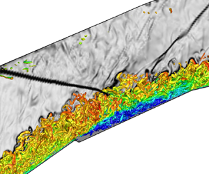
The four DNS utilized to study the flow in the ramp–isolator junction are visualized in figure 12, using an isolevel of Q-criterion, coloured by streamwise velocity. The ROCs of the faceted and notched junctions are shown in figure 12(a,c), respectively. The cowl SBLIs in the corresponding cases are shown in figure 12(b,d), respectively, using density-gradient contours on a spanwise plane. The two geometries exhibit key differences in several aspects of the flow, including, unsteady scales in the boundary layer, size of the separation bubble, structure of separation-induced compression waves emanating from the junction, and postinteraction boundary layer.

Figure 12. Flow structures identified using isolevel of Q-criterion, coloured with u-velocity: (a) ROC and (b) cowl SBLI for the faceted geometry. Panels (c,d) are the corresponding results for the notched geometry. Impinging and reflected shocks in the interaction region are visualized using density gradient magnitude ($\| \boldsymbol {\nabla } \rho \|$) in (b,d).

The mean flow fields of these four cases are compared in figure 13. The ${\boldsymbol {u}\boldsymbol {\cdot }\boldsymbol {\nabla } p}$ fields are utilized to effectively identify the compression and expansion zones, which appear as the red and blue fields, respectively. Streamlines are also included to indicate the turning of the flow due to these waves. The compression ramp shock is visible at the top left-hand corners. In the faceted ROC (figure 13a), the scenario is relatively simpler, where the flow turns towards the streamwise direction through two expansion fans. The notched ROC (figure 13c) displays a comparatively stronger expansion fan at the step edge, followed by a reattachment shock. Although not marked, a localized recirculation bubble exists between the expansion fan and reattachment shock.

Figure 13. The ${\boldsymbol {u}\boldsymbol {\cdot }\boldsymbol {\nabla } p}$ fields of all four cases: (a) ROC and (b) cowl SBLI for the faceted geometry. Panels (c,d) are the corresponding results for the notched geometry. Streamlines are also indicated, including the dividing streamlines for the SBLI cases. Important flow features are marked with numbers for SBLI cases.

The cowl SBLI cases are presented in figure 13(b,d). The impingement of the ramp shock on the cowl lip is evident near the top left-hand corners of the ${\boldsymbol {u}\boldsymbol {\cdot }\boldsymbol {\nabla } p}$ contour plots. Such a shock at lip condition ensures maximum mass flow capture with optimum total pressure recovery (Seddon & Goldsmith Reference Seddon and Goldsmith1999). The region of this computational boundary modelled as the no-slip wall is highlighted in black. The flow features are marked with respective numbers for clarity. The impinging cowl shock ${\bigcirc{\kern-6pt 1}}$ leads to boundary layer separation on the ramp surface of the baseline faceted case (figure 13b). The dividing streamline indicates the extent of the separation bubble, which has a length of $0.903 H_I$. The upstream end of the bubble is well-removed from the impinging cowl shock and creates a separation shock ${\bigcirc{\kern-6pt 3}}$ and affects the expansion fan ${\bigcirc{\kern-6pt 2}}$. The cowl shock continues downstream as a reflected shock ${\bigcirc{\kern-6pt 4}}$, followed by an expansion fan ${\bigcirc{\kern-6pt 5}}$ (created due to the decreasing thickness of the bubble). The separation shock and the reflected shock coalesce to form a single shock. A reattachment shock ${\bigcirc{\kern-6pt 6}}$ also exists downstream of the expansion fan, where the separation bubble terminates. Finally, the flow encounters the expansion fan ${\bigcirc{\kern-6pt 7}}$ at the isolator entrance. The interaction of the upstream expansion fan and the separated shock with the cowl shock leads to changes in respective wave angles. It has to be noted that the shocks and the expansion fans do not reflect back into the intake from the cowl-side wall at downstream locations due to the outflow conditions imposed there.

The SBLI over the notched junction (figure 13d) produces a larger separation bubble that originates from the step edge, and has a streamwise length of $1.141 H_I$. Since control of SBLI is a major objective of junction design, the notch depth adopted here is approximately $31\,\%$ of the incoming boundary layer. Under this condition, the small separation bubble at the notch (discussed in figure 13c) coalesces with the elongated bubble generated by the impinging shock. For smaller notch depths, the edge bubble and the SBLI bubble remain separated, making the flow very similar to the baseline faceted case. Based on studies by Li & Liu (Reference Li and Liu2019), it is important to have the impingement of the shock on the separated shear layer for effective control of SBLI. Comparing figure 13(b,d), it is evident that the notched junction eliminates the separation shock and significantly weakens the reflected shock ${\bigcirc{\kern-6pt 2}}$. The cowl shock impinging on a separated shear layer reflects predominantly as an expansion fan ${\bigcirc{\kern-6pt 3}}$. These features are consistent with the observations of Li & Liu (Reference Li and Liu2019), based on the study of an idealized BFS. The reattachment shock ${\bigcirc{\kern-6pt 4}}$ and the downstream expansion fan ${\bigcirc{\kern-6pt 5}}$ are similar between the notched and the faceted cases.

The cowl SBLI cases are now compared with corresponding results from the experiments in figure 14. Qualitative comparisons are made between the experimental shadowgraphs (figure 14a,c) and the second derivatives of the mean DNS density fields (figure 14b,d).

Figure 14. Comparison of Experimental and DNS shadowgraphs of SBLI flow fields: (a,b) faceted junction and (c,d) notched junction.

Flow features are marked using arrows in the images for ease of comparison. A good agreement is observed between the two flow fields for both the faceted and the notched cases. The simulated expansion fan downstream of the reflected shock, and the reattachment shock, match with that from the experiments of the faceted geometry (figure 14a,b). The most prominent flow features of the notched junction (figure 14c,d) are the expansion fans (as a reflection of cowl shock) and the reattachment shocks, which again show a good match between the experiments and the DNS. The experiment identifies a relatively shorter separation bubble at the faceted junction, which starts slightly downstream from the corner. The differences in separation length scales can be attributed to the lower Reynolds number utilized in the DNS (e.g. the effect of Reynolds number as discussed in Lin & Pauley (Reference Lin and Pauley1996)), as well as the three-dimensional effect in the experiments.

To quantitatively compare the flow fields from experiments and DNS, we provide wall-pressure plots in figure 15. Here, the spanwise and temporally averaged wall pressure from the DNS is compared with the temporally averaged centreline wall pressure measured on the intake floor. As the DNS was performed at $Re=40\,000$, the wall pressure from RANS simulations performed at $Re=400\,000$ is also included, to identify deviations in the high-fidelity simulations that are potentially driven by Reynolds number effects. In addition, to highlight the role of viscous effects, results from inviscid (Euler) simulations are also included.

Figure 15. Comparison of experimental and DNS wall pressures: (a) faceted junction and (b) notched junction. Corresponding Euler and RANS simulations are also included.

All simulations display very close agreement with the experimental results over the ramp, upstream to the ramp–isolator junction ($x < 9$). Wall pressure at the faceted junction (figure 15a) drops at the corner due to the upstream expansion fan. In the inviscid simulation, wall pressure remains nearly constant ($9 \le x \le 10$) until the cowl shock impinges at the junction, which raises the wall pressure at $x \sim 10$. It further remains constant, until the expansion fan at the isolator entrance ($x \sim 10.6$) brings it down. The interaction between the cowl shock and the floor boundary layer is moderately strong in the present case, with viscous effects inducing flow separation. This causes the pressure distribution predicted by RANS simulations and DNS to be significantly different from that in the inviscid simulation. The general trends in the RANS and DNS predictions are consistent with those in the experiment. The mismatch between the DNS and experimental curves is attributed to the low-Reynolds number effect, which results in a relatively larger separation bubble in the DNS. This is further supported by the observation that the RANS simulation at the experimental Reynolds number rectifies this mismatch and closely follows the experimental measurements at all locations, both within and outside the interaction region. The initial rise in wall-pressure ($9.3 < x < 10$) is due to the impinging/reflected shock, and the downstream pressure-rise ($10 < x < 10.7$) is induced by the reattachment shock. The downstream pressure drop through an expansion fan at the isolator entrance is visible in the viscous simulations as well.

In the case of the notched junction (figure 15b), viscous effects dominate at the ramp–isolator junction due to the flow separation induced by the step discontinuity. In supersonic BFS flows, prior studies have shown that the static pressure drops to lower levels in the base region due to expansion at the edge (Sfeir Reference Sfeir1966), but the same was not observed in the present scenario. However, as typically observed in BFS flows (Sfeir Reference Sfeir1966; Hartfield, Hollo & McDaniel Reference Hartfield, Hollo and McDaniel1993), the pressure is almost constant within the base region. The experimental and RANS pressure values at the junction continue to stay at almost the same level as the upstream flow, as there is only a marginal flow turning along the notch profile, which remains shielded from the outer inviscid flow by the bubble. The DNS pressure in the base region is lower than that in the experiments, but nonetheless, it follows the trend closely. Though a localized negative pressure gradient exists at the notch edge in the DNS, it does not propagate upstream, due to the turbulent nature of the incoming boundary layer (Sfeir Reference Sfeir1966). Post reattachment, the pressure rises ($10 < x < 10.7$) due to the reattachment shock, and drops downstream due to the expansion fan at the isolator entrance.

4.2. Dynamics of ramp–isolator junction

To quantify the dynamics of the ramp–isolator junction, we extract the PSD from wall-pressure fluctuations for the ROC and SBLI cases. Figure 16(a,c) show spectra of the ROC, while figure 16(b,d) contain spectra with the cowl SBLI. The logarithms of the PSD values are plotted in order to ensure clarity of the trends. The ramp flows in all four cases exhibit similar dynamics involving KH instabilities and subsequent transition to turbulence at $x \sim 6.5$, which is marked using the vertical dashed lines. However, each flow harbours distinct dynamics downstream of the ramp–isolator junction, depending on the geometry and characteristics of the SBLI. The faceted ROC displays mitigation of unsteadiness each time the flow expands (at the junction and the isolator entrance). As the flow accelerates through the expansion fan, it tends to relaminarize (Narasimha & Sreenivasan Reference Narasimha and Sreenivasan1973), resulting in a monotonic drop in PSD amplitudes. On the other hand, the notched ROC spectra first show a drop in unsteadiness at the upstream edge, followed by a peak and a decay as seen in figure 16(c), highlighted by an oval. This behaviour of the notched ROC is typical to BFS flows, where the oscillations peak immediately upstream of the reattachment, followed by a rapid decay (Eaton & Johnston Reference Eaton and Johnston1981). There is a subsequent drop in unsteadiness over the isolator floor due to the effect of the downstream expansion fan. In both the ROC, the flow enters the isolator floor with diminished unsteadiness, which is outside the range of levels plotted here.

Figure 16. Wall pressure spectra (log–PSD) of the ramp, junction and isolator flow fields: (a) faceted ramp only; (b) faceted ramp SBLI; (c) notched ramp only; and (d) notched ramp SBLI. The red dashed lines indicate the transition to turbulence.

As seen in figure 16(b,d), the flow upstream of the ramp–isolator junction for the SBLI cases is nominally similar in dynamics to the ROC cases discussed above. However, the boundary layer interactions with the cowl shock energize a broad spectral range. Unlike the ROC cases, unsteadiness generated at the junction largely persists into the isolator section, in spite of the attenuation due to the downstream expansion fan.

The dynamics of the ramp–isolator junctions with cowl SBLI are further evaluated in detail, in the context of near-wall flow features. These wall-pressure spectra are aligned with the corresponding numerical shadowgraphs in figure 17. To juxtapose the unsteady scales in the interaction regions with SBLI literature, we adopt the separation length in the respective cases to scale the spectra. The dividing streamlines are also marked to indicate the boundaries of the separation bubbles.

Figure 17. Wall pressure spectra (log–PSD) of junction SBLI: (a) Faceted and (b) Notched. Corresponding numerical shadowgraphs are also included for reference. The dotted line indicates the low-frequency peak in the faceted junction spectra. The dashed lines mark the reattachment locations. The dot-dashed lines mark the isolator start.

A prominent feature of the faceted junction spectra (figure 17a) is the low-frequency peak ($St_L = 0.03\unicode{x2013}0.04$) near the separation and the reattachment points. It corresponds to the shock motion related to bubble breathing and matches very well with the spectral estimates in previous studies (Touber & Sandham Reference Touber and Sandham2009; Aubard et al. Reference Aubard, Gloerfelt and Robinet2013). Since the separation bubble is relatively thinner in the faceted junction, the separated shear layer develops in close proximity to the wall surface. Therefore, the higher frequencies corresponding to shear layer instabilities ($St_L > 0.1$) are not excited until it is sufficiently thick ($x > 9.5$). The midfrequency component ($0.1 \le St_L \le 1$) corresponding to coherent fluctuations in the shear layer become prominent from $x \sim 9.5$. This has been attributed to KH instabilities that develop in the postinteraction shear layer of the bubble (Adler et al. Reference Adler, Gonzalez, Stack and Gaitonde2018). The interaction region of the cowl shock also generates fine-scale structures that populate the high-frequency content ($St_L > 1$). The drop in PSD amplitudes from the mid- to the high-frequency zone is consistent with the cascading effect. The bubble motion, KH instabilities of the shear layer, and the fine-scale structures contribute to the broadband content postreattachment ($10.1 \le x \le 10.6$). The attenuation effect of the expansion fan at the isolator entrance is most visible at higher frequencies, resulting in the dominance of low/low-midfrequency content ($St_L \le 0.4$) within the isolator boundary layer.

The wall-pressure spectrum of the notched junction (figure 17b) exhibits a different set of dynamics. The prominent low-frequency peak related to bubble breathing is absent near the separation point. Here, flow separation is initiated at the upstream geometric discontinuity of the notch, which effectively locks the streamwise movement of the separation point. The reattachment point is still free to move, and hence the low-frequency content is visible at this location. The separated shear layer originating from the notch edge thickens and amplifies instabilities relatively quickly. The corresponding high-frequency oscillations ($St_L > 1$) emerge close to the notch-edge, followed by the midfrequency content ($0.1 \le St_L \le 1$). Post reattachment ($10.2 \le x \le 10.6$), the midfrequency content dominates, while the low-frequency oscillations become weaker, compared with the faceted junction, where this trend was reversed. This suggests the dominance of shear layer dynamics driven by shedding from the separation bubble. The trend continues into the isolator, which primarily retains a selective band of midfrequency oscillations ($0.2 \le St_L \le 0.4$). The current analysis reveals that utilizing a notched junction enforces one-sided locking of the separation bubble movement, thereby almost eliminating the low-frequency oscillations near the separation point, and significantly attenuating those within the isolator.

To quantify the effects of junction geometry on the unsteadiness of inviscid features of the compression path, the root mean squared (r.m.s.) values of pressure fluctuations from the DNS are presented in figure 18. The r.m.s. contours extracted from the midspan plane (figure 18a,b) identify several regions of unsteadiness, including the compression wave from the external ramp surface directed towards the cowl lip. High levels of fluctuations exist near the shock waves, including in the inviscid regions and regions of interaction with the boundary layer, and the flow downstream of the reattachment. Near-wall fluctuations attenuate at the isolator entrance due to the expansion fan, but the unsteadiness in the reattachment shock sustains. Among the shocked regions, peak unsteadiness is visible in the cowl shock, in relation to the separation shock and the reattachment shock. The separation shock fluctuations are primarily driven by the low-frequency motion of the separation bubble at the faceted junction, and this component is eliminated in the notched junction, consistent with the spectral analysis discussed in figure 17. The reattachment shock oscillations have additional contributions from shear layer structures and turbulent fluctuations. To compare the unsteadiness between the two junctions, the r.m.s. pressures are extracted along the common midstream line (marked using solid lines in figure 18a,b) and plotted in figure 18(c). The flow unsteadiness upstream to the junction shows a hump near the compression ramp shock at $x \sim 7.5$. A good match of r.m.s. values indicates that the incoming flows of both junctions are identical, as expected. The largest peaks are observed near the cowl shock in both geometries. However, the cowl shock of the faceted junction has comparatively higher unsteadiness. Downstream of the cowl shock, relatively smaller peaks represent the separation shock, expansion fans and reattachment shocks.

Figure 18. The r.m.s. pressures of the ramp–isolator junction flow fields: (a) faceted; (b) notched; (c) comparison along the domain centreline. The red line indicates probe points for comparison.

Additional r.m.s. traces are reported in figure 19 for both geometries, aligned with the corresponding mean ${\boldsymbol {u}\boldsymbol {\cdot }\boldsymbol {\nabla } p}$ fields. For the faceted junction, these are shown in figure 19(a). The peak r.m.s. value drops from trace F1 to F2 due to the interaction of the impinging cowl shock with the expansion fan. Such interaction of the impinging shock is absent in typical SBLI studies. The peak value increases again (trace F3) where the cowl shock interacts with the separation shock. The r.m.s. pressure peak is highest along trace F4 where the cowl shock interacts with the floor boundary layer. Similarly, around the notched junction (figure 19b), the peak r.m.s. pressure drops from trace N1 to N2 due to the interaction with the expansion fan originating at the edge of the notch. The cowl shock unsteadiness rises downstream and is highest near the interaction region (trace N3), close to the maximum thickness of the bubble.

Figure 19. The r.m.s. pressures along the traces of (a) faceted and (b) notched junction. The ${\boldsymbol {u}\boldsymbol {\cdot }\boldsymbol {\nabla } p}$ fields aligned with the corresponding r.m.s. pressure distributions are also shown.

To obtain the spatiotemporal forms of the unsteady features identified in wall spectra, we extract the relevant harmonics using DMD, from the streamwise velocity fluctuations on the midspan plane. Three modes are discussed in detail for each junction geometry, that are representative of the low-, mid- and high-frequency bands identified in figure 17.

The low-frequency mode is shown first in figure 20. The mean field is also added to the corresponding fluctuations to visualize the bubble-breathing motion that this mode represents. The bubble in the faceted junction is at its largest size in figure 20(a). The bubble shrinks as it sheds mass into the downstream flow, with the smallest size in figure 20(c). Subsequent entertainment of mass, and bubble dilation, are seen in figure 20(d). This breathing behaviour has been observed in experiments (Piponniau et al. Reference Piponniau, Dussauge, Debieve and Dupont2009) and numerical simulations (Aubard et al. Reference Aubard, Gloerfelt and Robinet2013) of canonical flat plate boundary layers with shock-induced separation. As shown by Piponniau et al. (Reference Piponniau, Dussauge, Debieve and Dupont2009), the streamwise movements of the bubble are linked with its contractions and dilatations in case of canonical impinging SBLI. The change in bubble size is a result of mass, momentum and vorticity transfer between the recirculating region and the outside flow. The mixing layer entrainment also plays an important role in this process.

Figure 20. Contours of the low-frequency DMD modes in the (a–d) faceted and (e–h) notched junctions shown at equally spaced phase-intervals. The modes correspond to $St_L = 0.041$ and $St_L = 0.081$ for the faceted and notched cases, respectively. The mean flow field is added to the fluctuations. Here (a) $\phi =0$; (b) $\phi ={\rm \pi} /2$; (c) $\phi ={\rm \pi}$; (d) $\phi =3{\rm \pi} /2$; (e) $\phi =0$; (f) $\phi ={\rm \pi} /2$; (g) $\phi ={\rm \pi}$; (h) $\phi =3{\rm \pi} /2$.

The low-frequency behaviour at the notched junction is considerably different from that in the faceted junction, and is shown in figure 20(e–h). The breathing motion still exists, as the entrainment mechanism is active. However, in notched geometry, it primarily affects the downstream portion of the bubble at $x \sim 10$, consistent with the observations in the wall spectra (figure 17b). The dilation-phase of the bubble in this case is from $\phi = {\rm \pi}/2$ to $\phi = 3{\rm \pi} /2$. As the notch effectively locks the separation, the separation point has no effect of breathing motions. However, the reattachment point is influenced by bubble breathing, with its most upstream location corresponding to the smallest bubble size, and vice versa. The impact of bubble-breathing on variations in its streamwise location will be further evaluated in the context of separation and reattachment locations, later in this discussion.

The midfrequency modes for both geometries are shown in figure 21, along with the binary ${\boldsymbol {u}\boldsymbol {\cdot }\boldsymbol {\nabla } p}$ fields superimposed to indicate the mean states of cowl shock and dividing streamline. Figure 21(a–d) clearly show the shedding of structures from the shear layer, which confirms their contribution to the midfrequency band of the faceted junction. The shedding results from KH instability waves, which are typically observed around laminar separation bubbles (e.g. Simoni et al. Reference Simoni, Lengani, Ubaldi, Zunino and Dellacasagrande2017; Rodríguez et al. Reference Rodríguez, Gennaro and Souza2018). The structures convect downstream and are attenuated across the expansion fan at the isolator corner. The midfrequency mode in the notched junction (figure 21e–h) has a different spatial form, with the shed vortical structures being relatively distorted. Since the shear layer originating from the notch's edge is well-developed, the notched junction has similarities with typical shock–shear layer interactions. For example, such ‘distorting’ vortical structures were observed by Karthick (Reference Karthick2021) in a supersonic cavity shear layer, interacting with an impinging shock. The oscillations amplify after the shedding, and convect downstream into the isolator with strong amplitudes, even after passing through the expansion fan. This justifies the presence of a strong midfrequency component in the wall-pressure spectrum of the notched junction (figure 17b).

Figure 21. Contours of the midfrequency DMD modes in the (a–d) faceted and (e–h) notched junctions shown at equally spaced phase-intervals. The modes correspond to $St_L = 0.526$ and $St_L = 0.395$ for the faceted and notched cases, respectively. The mean states of the corresponding cowl shocks and dividing streamlines are also indicated. Here (a) $\phi =0$; (b) $\phi ={\rm \pi} /2$; (c) $\phi ={\rm \pi}$; (d) $\phi =3{\rm \pi} /2$; (e) $\phi =0$; (f) $\phi ={\rm \pi} /2$, (g) $\phi ={\rm \pi}$; (h) $\phi =3{\rm \pi} /2$.

Corresponding results for the high-frequency modes are shown in figure 22. The high-frequency mode of the faceted junction (figure 22a–d) identifies the growth of vortical structures within the shear layer, from the separation point to the shock-impingement location. The PSD contours (shown earlier in figure 17a) also confirm the amplification of unsteadiness at medium and high-frequencies in this region ($x \sim 9.5$). Post interaction with the shock, the amplified structures disintegrate within the adverse-pressure gradient region, contributing to the fine-scale turbulence generated at the isolator entrance. The high-frequency mode of the notched junction (figure 22e–h) is very similar to that of the faceted junction. The similarity between these modes suggests the universality of fine-scale spatiotemporal scales in SBLI, in spite of differences in the thickness of the mean shear layers, and their relative displacements from the wall.

Figure 22. Contours of the high-frequency DMD modes in the (a–d) faceted and (e–h) notched junctions shown at equally spaced phase-intervals. The modes correspond to $St_L = 2.03$ and $St_L = 1.95$ for the faceted and notched cases, respectively. The mean states of the corresponding cowl shocks and dividing streamlines are also indicated. Here (a) $\phi =0$; (b) $\phi ={\rm \pi} /2$; (c) $\phi ={\rm \pi}$; (d) $\phi =3{\rm \pi} /2$; (e) $\phi =0$; (f) $\phi ={\rm \pi} /2$; (g) $\phi ={\rm \pi}$; (h) $\phi =3{\rm \pi} /2$.

A quantitative comparison of the effects of various frequency bands on separation bubble dynamics is presented in figure 23. The displacement of the point of separation from its time-averaged position is shown in figure 23(a) for both geometries. Results are included for the three bands of frequencies discussed above. Corresponding results for the reattachment location are plotted in figure 23(b). It is evident from figure 23(a) that the separation point in the notched junction experiences negligible fluctuations for all bands of frequencies, compared with that in the faceted junction. In the faceted junction, peak oscillations of the separation point are induced by the low-frequency component. Corresponding mid- and high-frequency oscillations are lower by an order of magnitude. This is because the upstream portion of the bubble harbours a nascent shear layer in which the associated instabilities have not amplified yet, compared with downstream locations.

Figure 23. Comparison of streamwise oscillations of (a) separation point and (b) reattachment point caused by various bands of frequencies in the faceted and notched junctions.

The reattachment point has relatively amplified unsteadiness as seen in figure 23(b), for all bands of frequencies. While the high-frequency dynamics still have the lowest amplitudes, the low and midfrequency dynamics have comparable effects. An interesting observation here is that the midfrequency oscillations have higher amplitudes than the low-frequency oscillations in both geometries, indicating the significance of shear layer structures in impacting SBLI in inlets. The relative dominance of midfrequency oscillations (of the reattachment point) over other frequency bands is most evident in the notched junction. The spatial form of this mode (figure 21e–h) had earlier identified these enhanced midfrequency oscillations to cause the shedding of vortical structures that persist in the isolator. This phenomenon could energize the boundary layer through cross-stream mixing of near-wall flow, assisting an efficient compression process. Unlike the separation point, the reattachment point oscillations of the faceted and notched junctions have similar amplitudes at low-frequency. However, their qualitative nature is different. The faceted junction displays symmetric bubble oscillations, whereas those in the notched geometry are asymmetric with relatively longer periods of bubble dilation, and a rapid contraction.