


1. Introduction
One of the most striking features of turbulent geophysical flows is the emergence of persistent coherent vortices that thrive in seemingly hostile environments for periods that greatly exceed their typical turnaround time scales. Known examples of long-lived geophysical vortices include the Great Red Spot of Jupiter, as well as the Gulf Stream and Agulhas rings of the Earth's oceans. The remarkable durability of oceanic vortices is borne out by direct oceanographic measurements (e.g. Robinson Reference Robinson1983; Olson Reference Olson1991) and quantified by more recent satellite-based analyses (Chelton, Schlax & Samelson Reference Chelton, Schlax and Samelson2011; Samelson, Schlax & Chelton Reference Samelson, Schlax and Chelton2014). Several case studies show that coherent vortices can exist for up to four years, translating during their lifetimes over distances of thousands of kilometres from their points of origin (Chen & Han Reference Chen and Han2019). The ability of coherent vortices to transport distinct physical, biological and chemical properties across ocean basins makes it critical to determine their role in lateral mixing. Meeting this objective, in turn, demands a full understanding of their dynamics, stability and propagation mechanisms.
Coherent mesoscale vortices in the ocean attracted continuous interest from the geophysical community for at least half of a century and their basic properties are well documented. In particular, much attention in oceanographic literature has been paid to vortex rings, which represent pinched-off meanders of major ocean currents (e.g. Olson Reference Olson1991). The ocean rings are typically circular isolated structures with vanishing far-field circulation. They are characterized by the distinct vorticity distribution with the inner core containing vorticity of a certain sign and the annulus of opposite-sign vorticity. Such patterns are often described as ‘shielded’ and used in theoretical and numerical studies of coherent vortices (e.g. Carton Reference Carton2001; Sokolovskiy & Verron Reference Sokolovskiy and Verron2014). The conceptual model of the ocean rings as shielded vortices is supported by the direct oceanographic measurements (e.g. Olson Reference Olson1991; Fratantoni, Johns & Townsend Reference Fratantoni, Johns and Townsend1995). Observations indicate that the azimuthal velocity in rings first increases from zero at their centres to the maximal velocity value of ~1 m s−1 at the radius of  ${r_{max}} = 50-100\,\textrm{km}$. Further from the centre, the velocity reduces, effectively vanishing at a finite external radius, exceeding
  ${r_{max}}$ by a factor of 2–3.
The propagation speeds of ocean rings are of the order of several centimetres per second, which is much less than their maximal azimuthal velocities. It should also be emphasized that rings are not merely advected by large-scale currents but often exhibit self-propagation tendencies. For instance, fully developed Gulf Stream rings tend to drift to the West, even though the background flow at the level of shallow vortices is eastward. One of the mechanisms for self-propagation is associated with the variation of the planetary vorticity with latitude, known as the beta-effect. The beta-effect acting on a circular vortex naturally induces the dipolar component – so-called beta gyre – which ultimately leads to a systematic westward drift (e.g. Sutyrin & Flierl Reference Sutyrin and Flierl1994; Flór & Eames Reference Flór and Eames2002). However, the beta-effect is not the only source of dipolar components in geophysical eddies. The dipolar pattern can be produced by the interaction with other coherent structures or it can form during the same process that generated the vortex in the first place (e.g. Stern & Radko Reference Stern and Radko1998; Radko Reference Radko2008). Once introduced, the dipolar component can be retained by a vortex for long periods, strongly affecting its dynamics and trajectory (e.g. Radko & Stern Reference Radko and Stern1999, Reference Radko and Stern2000).
Since the dipolar component of geophysical vortices is expected to be relatively weak, its presence can be effectively masked in observations by the dominant circularly symmetric pattern. Thus, an appropriate conceptual model for the ocean rings should represent a long-lived quasi-monopolar structure capable of persistent drift relative to the background large-scale flow. Unfortunately, the number of exact solutions that can capture these characteristics is surprisingly limited. A distinct line of research stems from the classical solution of the two-dimensional Euler equations (Lamb Reference Lamb1895) characterized by the linear relation between the vorticity and the streamfunction. The original Lamb's solution represents a purely dipolar structure and therefore its ability to describe typical oceanic rings is questionable. This result was independently obtained and substantially generalized by Chaplygin (Reference Chaplygin1903), who discovered a class of solutions representing a superposition of Lamb's dipole and a circularly symmetric pattern, often referred to as a ‘rider’. A concise account of Chaplygin's work in this area can be found in Meleshko & van Heijst (Reference Meleshko and van Heijst1994). Several extensions of such ‘modon-with-the-rider’ solutions have been proposed, which incorporate the effects of stratification and the beta-effect (Berestov Reference Berestov1979; Flierl et al. Reference Flierl, Larichev, McWilliams and Reznik1980). The Achilles heel of these models is their strong instability in the oceanographically relevant quasi-monopolar regime, where the amplitude of the circular rider exceeds the dipolar component. Numerical simulations (e.g. Swenson Reference Swenson1987) reveal that the instability of dominant ‘riders’ results in the destruction of the initial configuration, precluding their use as models of oceanic rings.
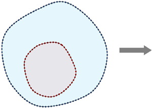
An alternative approach to the problem involves the development of asymptotic, rather than exact, quasi-monopolar solutions that remain coherent for long periods. Particularly relevant for our study is the asymptotic model representing two circular overlapping patches of piecewise uniform vorticity (Stern Reference Stern1987; Stern & Radko Reference Stern and Radko1998). If the net vorticity is zero, a small separation between the centres of the inner and outer patches (figure 1) introduces a weak but persistent dipolar component. This dipole is largely masked by the predominantly monopolar circulation, but still causes a systematic drift of the entire structure. Numerical simulations confirm that vortices constructed in this manner are capable of self-propagation over distances that greatly exceed their sizes. Such asymptotic solutions can be conveniently used to study interactions of self-propagating vortices with distant currents, topographic features, basin boundaries or other eddies (e.g. Stern & Radko Reference Stern and Radko1998; Radko Reference Radko2008). Nevertheless, a more fundamental theoretical question remains unanswered: are there any exact solutions of two-dimensional Euler equations that (i) take the form of rectilinearly propagating quasi-monopolar eddies and (ii) are sufficiently stable to maintain their structure and intensity for lengthy periods in the presence of finite-amplitude perturbations?

Figure 1. Schematic diagram illustrating the structure of the sought-after V-states.
The lack of definitive answers to this question for quasi-monopolar vortices is perhaps surprising given the abundance of the corresponding dipolar models (e.g. Pierrehumbert Reference Pierrehumbert1980; Wu, Overman & Zabusky Reference Wu, Overman and Zabusky1984; Dritschel Reference Dritschel1995; Makarov & Kizner Reference Makarov and Kizner2011). Exact stable dipolar solutions were obtained for both symmetric and non-symmetric partners, moving either straight or in circles. These dipolar solutions with piecewise uniform vorticity distribution are undoubtedly interesting in their own right. However, the present investigation, which is largely motivated by the observations of ocean rings, is focused on quasi-monopolar configurations. The latter models are considerably different in terms of vortex structure, dynamics and the mechanism of motion relative to the ambient fluid.
The algorithm used in our study to obtain rectilinearly propagating solutions, which are commonly referred to as translating V-states, is based on the well-known contour-dynamics (CD) equations (Overman & Zabusky Reference Overman and Zabusky1982; Stern & Pratt Reference Stern and Pratt1985). The CD model expresses the velocity field induced by each uniform vorticity patch as a line integral along its boundary. The key strength of the CD model, compared to algorithms utilizing stationary two-dimensional grids, is its ability to perform temporal integrations of fully inviscid equations of motion.
In the present study, we first (§ 2) use the CD formulation to find translating V-states represented by two overlapping patches, as illustrated in figure 1. The exploration of the parameter space that follows (§ 3) indicates that such solutions exist only for relatively low values of the target vortex propagation speed U. The linear stability analysis of the translating V-states, presented in § 4, indicates that all such solutions are formally unstable. Nevertheless, some of the solutions – particularly those with small inner vorticity patches – are characterized by very low growth rates. This finding, in turn, suggests that the instability does not necessarily lead to the destruction of the obtained V-states in the presence of weak perturbations. A series of integrations of nonlinear evolutionary CD equations in § 5 confirm that quasi-monopolar vortices with small inner cores are robust and capable of propagation over distances greatly exceeding their size while maintaining their structure and intensity. In § 6, we argue that the proposed solutions can be readily generalized to incorporate the beta-effect and apply our findings to observations of ocean rings. We summarize our findings and draw conclusions in § 7.
2. Formulation
Our investigation attempts to identify and analyse exact rectilinearly propagating two-dimensional solutions taking the form of quasi-monopolar eddies with zero net vorticity. These solutions are sought in the form of a superposition of two piecewise uniform vorticity patches, arranged in the manner shown in figure 1. The governing Euler equations for this configuration are non-dimensionalized using the effective eddy radius  $r_1^\ast{\equiv} \sqrt {S_1^\ast{/}\pi } $ as a unit of length and
  ${(\varsigma _1^\ast )^{ - 1}}$ as a time unit, where
  $S_1^\ast $ and
  $\varsigma _1^\ast $ are, respectively, the dimensional area and vorticity of the outer patch. This non-dimensionalization is equivalent to setting the area of the outer patch to
  $\pi $ and its vorticity to unity.
The requirement of zero net vorticity is satisfied by relating the non-dimensional vorticity  $({\varsigma _2})$ and the area (S 2) of the inner patch as follows:
 \begin{equation}{S_2}{\varsigma _2} + \pi = 0.\end{equation}
Therefore, the effective radius of the inner contour is  ${r_2} \equiv \sqrt {{S_2}/\pi } = \sqrt { - \varsigma _2^{ - 1}} $. The resulting system is analysed using the CD model (Overman & Zabusky Reference Overman and Zabusky1982; Stern & Pratt Reference Stern and Pratt1985), in which the velocity fields induced by each vorticity patch are expressed in terms of boundary integrals
 \begin{equation}\left.
{\begin{aligned} u(x,y) & =- \dfrac{\varsigma }{{4\pi
}}\dfrac{\partial }{{\partial y}}\iint_S {\ln ({{(x -
x^{\prime})}^2} + {{(y -
y^{\prime})}^2})\,\textrm{d}x^{\prime}\,\textrm{d}y^{\prime}}
\\ & =\dfrac{\varsigma }{{4\pi }}\oint_C {\ln ({{(x -
X)}^2} + {{(y - Y)}^2})\,\textrm{d}X} , \\
v(x,y) & =\dfrac{\varsigma }{{4\pi }}\dfrac{\partial }{{\partial
x}}\iint_S {\ln ({{(x - x^{\prime})}^2} + {{(y -
y^{\prime})}^2})\,\textrm{d}x^{\prime}\,\textrm{d}y^{\prime}}
\\ & =\dfrac{\varsigma }{{4\pi }}\oint_C {\ln ({{(x -
X)}^2} + {{(y - Y)}^2})\,\textrm{d}Y,} \end{aligned}}
\right\}\end{equation}
\begin{equation}\left.
{\begin{aligned} u(x,y) & =- \dfrac{\varsigma }{{4\pi
}}\dfrac{\partial }{{\partial y}}\iint_S {\ln ({{(x -
x^{\prime})}^2} + {{(y -
y^{\prime})}^2})\,\textrm{d}x^{\prime}\,\textrm{d}y^{\prime}}
\\ & =\dfrac{\varsigma }{{4\pi }}\oint_C {\ln ({{(x -
X)}^2} + {{(y - Y)}^2})\,\textrm{d}X} , \\
v(x,y) & =\dfrac{\varsigma }{{4\pi }}\dfrac{\partial }{{\partial
x}}\iint_S {\ln ({{(x - x^{\prime})}^2} + {{(y -
y^{\prime})}^2})\,\textrm{d}x^{\prime}\,\textrm{d}y^{\prime}}
\\ & =\dfrac{\varsigma }{{4\pi }}\oint_C {\ln ({{(x -
X)}^2} + {{(y - Y)}^2})\,\textrm{d}Y,} \end{aligned}}
\right\}\end{equation}where X and Y represent the coordinates of points located at the contour C. The expressions in (2.2) can be further reduced (e.g. Dritschel Reference Dritschel1986) to
 \begin{equation}\left. {\begin{aligned} {u = \dfrac{\varsigma }{{2\pi }}\oint_C {({{\cos
}^2}\theta \,\textrm{d}X + \cos \theta \sin \theta
\,\textrm{d}Y)} ,}\\ {v = \dfrac{\varsigma }{{2\pi
}}\oint_C {(\cos \theta \sin \theta \,\textrm{d}X + {{\sin
}^2}\theta \,\textrm{d}Y)} ,} \end{aligned}}
\right\}\end{equation}
\begin{equation}\left. {\begin{aligned} {u = \dfrac{\varsigma }{{2\pi }}\oint_C {({{\cos
}^2}\theta \,\textrm{d}X + \cos \theta \sin \theta
\,\textrm{d}Y)} ,}\\ {v = \dfrac{\varsigma }{{2\pi
}}\oint_C {(\cos \theta \sin \theta \,\textrm{d}X + {{\sin
}^2}\theta \,\textrm{d}Y)} ,} \end{aligned}}
\right\}\end{equation}where
 \begin{equation}\cos \theta = \frac{{x - X}}{{\sqrt {{{(x - X)}^2} + {{(y - Y)}^2}} }},\quad \sin \theta = \frac{{y - Y}}{{\sqrt {{{(x - X)}^2} + {{(y - Y)}^2}} }}.\end{equation}
To express the integrals in (2.3) in terms of a single independent quantity, we introduce the location variable s, defined over the interval  $0 \le s \le 1$. As s increases from zero to unity, the corresponding point with coordinates X(s) and Y(s) makes a full revolution along the contour C in the positive (counterclockwise) direction. Thus, the CD equations (2.3) reduce to definite integrals in s
 \begin{equation}\left. {\begin{aligned} {u = \dfrac{\varsigma }{{2\pi }}\int_0^1 {\left(
{{{\cos }^2}\theta \dfrac{{\textrm{d}X}}{{\textrm{d}s}} +
\cos \theta \sin \theta
\dfrac{{\textrm{d}Y}}{{\textrm{d}s}}} \right)\textrm{d}s,}
}\\ {v = \dfrac{\varsigma }{{2\pi }}\int_0^1 {\left( {\cos
\theta \sin \theta \dfrac{{\textrm{d}X}}{{\textrm{d}s}} +
{{\sin }^2}\theta \dfrac{{\textrm{d}Y}}{{\textrm{d}s}}}
\right)\textrm{d}s} .} \end{aligned}}
\right\}\end{equation}
\begin{equation}\left. {\begin{aligned} {u = \dfrac{\varsigma }{{2\pi }}\int_0^1 {\left(
{{{\cos }^2}\theta \dfrac{{\textrm{d}X}}{{\textrm{d}s}} +
\cos \theta \sin \theta
\dfrac{{\textrm{d}Y}}{{\textrm{d}s}}} \right)\textrm{d}s,}
}\\ {v = \dfrac{\varsigma }{{2\pi }}\int_0^1 {\left( {\cos
\theta \sin \theta \dfrac{{\textrm{d}X}}{{\textrm{d}s}} +
{{\sin }^2}\theta \dfrac{{\textrm{d}Y}}{{\textrm{d}s}}}
\right)\textrm{d}s} .} \end{aligned}}
\right\}\end{equation}Another advantage of expressing governing equations in terms of s, is that the periodicity of X(s) and Y(s) makes it possible to conveniently evaluate derivatives and integrals using the Fourier transform in s. In particular,
 \begin{equation}\frac{{\textrm{d}(X,Y)}}{{\textrm{d}s}} = \int_{ - \infty }^\infty {\textrm{i}k(\tilde{X},\tilde{Y})\,{\textrm{e}^{ - \textrm{i}ks}}\,\textrm{d}k} ,\end{equation}
where  $\tilde{X}(k)$ and
  $\tilde{Y}(k)$ are the Fourier images of X and Y. In the numerical implementations, we use fast Fourier transform as a means of converting variables between physical and spectral spaces. The adoption of the Fourier series for the evaluation of derivatives and integrals allows us to maintain the spectral accuracy of the proposed algorithms. Yet another benefit of spectral representation is that any desired shift of points around the contour
  $(s \to s + \varDelta )$ is trivially accomplished by multiplying the Fourier images by
  ${\textrm{e}^{\textrm{i}k\varDelta }}$. A minor drawback of using the spectral method in the CD calculations is that the evaluation of velocities requires
  ${\propto} {n^2}\,\ln \,n$ operations, where n is the number of points assigned to each contour. Therefore, the model is less efficient than its finite-difference counterparts, which require
  ${\propto} {n^2}$ operations. However, our configuration (figure 1) includes only two contours
  $({n_C} = 2)$ and therefore the calculation speed does not represent a significant constraint in the following analyses.
The numerical implementation of the CD-based algorithm is governed by the selection of a specific discretization scheme. In the following calculations, each vorticity patch is defined by specifying a finite number of grid points located at its boundary (C)
 \begin{equation}{X^{(i)}} = X({s^{(i)}}),\quad {Y^{(i)}} = Y({s^{(i)}}),\quad {s^{(i)}} = (i - 1)\varDelta s,\quad i = 1,2, \ldots ,n,\end{equation}
where  $\varDelta s = 1/n$. The grid points
  $({X^{(i)}},{Y^{(i)}})$ can be distributed along the contour C in many ways, and the choice of the most appropriate discretization is by no means obvious. In the proposed model, we adopt the equidistant distribution scheme by insisting that
 \begin{equation}\frac{{\textrm{d}L}}{{\textrm{d}s}} \equiv \sqrt {{{\left( {\frac{{\textrm{d}X}}{{\textrm{d}s}}} \right)}^2} + {{\left( {\frac{{\textrm{d}Y}}{{\textrm{d}s}}} \right)}^2}} = \textrm{const}\textrm{.} = L.\end{equation}
We assume that the condition (2.8) is satisfied at each grid point and therefore  ${ {\textrm{d}L/\textrm{d}s} |_{s = {s^{(i)}}}} = L$, where
  $i = 1,2, \ldots ,n$ and L is the length of the contour C.
The implementation of the equidistant scheme in the following model is simplified by introducing the orientation variable  $\varphi $, such that
 \begin{equation}\cos \varphi = \frac{1}{L}\frac{{\textrm{d}X}}{{\textrm{d}s}},\quad \sin \varphi = \frac{1}{L}\frac{{\textrm{d}Y}}{{\textrm{d}s}}.\end{equation}
The pattern of  $\varphi (s)$ effectively controls the shape of the contour. Given the values of the orientation variable at each grid point
  ${\varphi ^{(i)}} = \varphi ({s^{(i)}})$ and the contour length L, the discretized versions of equations (2.9a,b) can be solved for
  ${X^{(i)}}$ and
  ${Y^{(i)}}$ using the Fourier transform in s. The resulting solutions are defined up to constants. These constants of integration can be expressed, for instance, in terms of the mean coordinates
  $(\bar{X},\bar{Y})$ along the contour, where
 \begin{equation}\bar{X} \equiv \frac{1}{n}\sum\limits_{i = 1}^n {{X^{(i)}}} ,\quad \bar{Y} \equiv \frac{1}{n}\sum\limits_{i = 1}^n {{Y^{(i)}}} .\end{equation}
Thus, in summary, each contour in the presented model is fully defined by (i) n values of the orientation variable at grid points  ${\varphi ^{(i)}}$, (ii) the contour length L and (iii) the mean coordinates
  $(\bar{X},\bar{Y})$. It should be noted, however, that
  ${\varphi ^{(i)}}$ values are not entirely independent. The periodicity of X(s) and Y(s) implies that the right-hand side of (2.9a,b) would vanish after the integration in s and therefore
 \begin{equation}\int_0^1 {\cos \varphi \,\textrm{d}s} = 0,\quad \int_0^1 {\sin \varphi \,\textrm{d}s} = 0.\end{equation}
The final restriction that we impose on the sought-after solution is that the area of the outer contour is equal to  $\pi ,$ which arises from the adopted non-dimensionalization scheme. This condition is expressed as
 \begin{equation}{S_1} = \oint_{{C_1}} {{X_1}} \textrm{d}{Y_1} = \int_0^1 {{X_1}} \frac{{\textrm{d}{Y_1}}}{{\textrm{d}s}}\textrm{d}s = \pi .\end{equation}
 Based on formulation (2.5)–(2.12), we propose the following algorithm that computes rectilinearly propagating two-contour solutions. First, the number of controlling parameters is reduced by assuming that (i) the motion of the vortex as a whole is in the positive x-direction, and (ii) the mean coordinates of the inner contour are zero:  $({\bar{X}_2},{\bar{Y}_2}) = (0,0)$. Neither assumption leads to the loss of generality. Next, an explicit condition for rectilinear propagation is obtained by performing calculations in the frame of reference associated with the moving vortex, in which the advective velocity becomes
 \begin{equation}{\boldsymbol{v}_{new}} = (u - U,v),\end{equation}
where U is the vortex speed. Each vorticity patch is stationary in the moving coordinate system as long as the velocity at its boundary (C) is directed along it. This condition is concisely expressed as
 \begin{equation}{\boldsymbol{v}_{new}}\boldsymbol{\cdot }\boldsymbol{n} = 0,\end{equation}
where  $\boldsymbol{n}$ is the unit vector oriented perpendicular to the contour C
 \begin{equation}\boldsymbol{n} = \frac{{\left( {\frac{{\textrm{d}Y}}{{\textrm{d}s}}, - \frac{{\textrm{d}X}}{{\textrm{d}s}}} \right)}}{{\sqrt {{{\left( {\frac{{\textrm{d}X}}{{\textrm{d}s}}} \right)}^2} + {{\left( {\frac{{\textrm{d}Y}}{{\textrm{d}s}}} \right)}^2}} }}.\end{equation}
The numerical implementation of this algorithm requires the discretization of (2.14) at both contours. One of the principles used in choosing an appropriate discretization is that the number of quantities representing the system (input variables) matches the number of conditions imposed on the solution (M). The input variables comprise of  $\varphi _1^{(i)}\;(i = 1,2, \ldots ,{n_1})$,
  $\varphi _2^{(i)}\;(i = 1,2, \ldots ,{n_2})$, L 1, L 2,
  ${\bar{X}_1}\,$ and
  ${\bar{Y}_1},$ which brings their total number to
  $N = {n_1} + {n_2} + 4\,.$ We insist that condition (2.14) is satisfied at m 1 and m 2 equidistant points at the outer and inner contours respectively. Also enforced are the periodicity conditions (2.11a,b) on X and Y for both contours and the area constraint (2.12) on the outer contour. Therefore, the number of conditions imposed on the solution is
  $M = {m_1} + {m_2} + 5$. The requirement
  $M = N$ is satisfied by using
  ${m_1} = {n_1}$ and
  ${m_2} = {n_2} - 1$. As a result, the problem of finding propagating V-states reduces to solving a system of N nonlinear equations with N unknowns. The latter task is accomplished by employing the iterative Trust-Region algorithm (available in the Matlab library as the function ‘fsolve.m’) which minimizes the quadratic error norm of trial solutions. The inability of the algorithm to find a solution with the error of less than
  ${10^{ - 20}}$ after 10 000 iterations is viewed as an indication that steadily propagating configurations do not exist for a given set of controlling parameters (U and r 2).
3. Propagating solutions
Figure 2(a) presents an example of a translating V-state obtained for the target velocity of  $U = 0.02$ and the effective inner radius of
  ${r_2} = 0.5$ using the procedure described in § 2. The number of grid points in this calculation is
  $({n_1},{n_2}) = (256,128)$. Doubling the number of grid points results in the solution that is nearly identical to the one shown in figure 2(a), and so does halving
  $({n_1},{n_2})$. This agreement instils confidence that our results are robust and largely independent of resolution. The configuration used to initiate the iterative search for a steady solution consists of two concentric circular patches and the corresponding steady state (figure 2a) is characterized by a slight shift of the outer contour in the y-direction. This shift introduces the dipolar component of vorticity that propels the entire vortex in the x-direction (e.g. Stern & Radko Reference Stern and Radko1998).

Figure 2. Typical translating V-states. (a) The quasi-monopolar solution obtained for the target velocity  $U = 0.02$. (b) The dipolar solution obtained for
  $U = 0.2$. In both cases,
  ${r_2} = 0.5$.
It should be mentioned that a completely different class of solutions can be obtained for the same parameters (U and r 2) by changing the initial state for the iterative algorithm. For instance, figure 2(b) shows a typical V-state realized when the search is initiated by two non-overlapping circular vorticity patches. These solutions can be described as asymmetric dipoles. Such dipolar V-states have already received much attention in fluid-dynamical literature (e.g. Pierrehumbert Reference Pierrehumbert1980; Dritschel Reference Dritschel1995; Makarov & Kizner Reference Makarov and Kizner2011). However, motivated by geophysical applications, we focus our investigation primarily on quasi-monopolar vortices exemplified by the state in figure 2(a).
The ability of isolated vortices to propagate over large distances is directly linked to the well-known (e.g. Saffman Reference Saffman1992) principle of impulse conservation. This principle states that, in the absence of external forcing, the first moments of vorticity are conserved:
 \begin{equation}\left. {\begin{aligned} {\dfrac{{\textrm{d}{Q_x}}}{{\textrm{d}t}} = 0,}\,\,{Q_x} &= \iint {x\varsigma \,\textrm{d}x\,\textrm{d}y} ,\\ {\dfrac{{\textrm{d}{Q_y}}}{{\textrm{d}t}} = 0,}\,\,{Q_y} &= \iint {y\varsigma \,\textrm{d}x\,\textrm{d}y} .\end{aligned}} \right\}\end{equation}
For the piecewise uniform configuration considered in our study (figure 1), the vorticity moments in (3.1) reduce to
 \begin{equation}({Q_x},{Q_y}) = \pi ({X_{C1}} - {X_{C2}},{Y_{C1}} - {Y_{C2}}),\end{equation}
where  $({X_{C1}},{Y_{C1}})$ and
  $({X_{C2}},{Y_{C2}})$ represent the centroids of the outer and inner vorticity patches respectively
 \begin{equation}{X_{Cj}} = \frac{1}{{{S_j}}}\iint_{{S_j}} {x\,\textrm{d}x\,\textrm{d}y} ,\quad {Y_{Cj}} = \frac{1}{{{S_j}}}\iint_{{S_j}} {y\,\textrm{d}x\,\textrm{d}y} ,\quad j = 1,2.\end{equation}
The area integrals in (3.3a,b) can be readily expressed in terms of contour integrals using Green's theorem and, ultimately, reduced to the definite integrals in s
 \begin{equation}{X_{Cj}} = \frac{\displaystyle{\int_0^1 {\frac{\displaystyle{X_j^2}}{2}\frac{{\textrm{d}{Y_j}}}{{\displaystyle\textrm{d}s}}\,\textrm{d}s} }}{{\displaystyle\int_0^1 {{X_j}\frac{\displaystyle{\textrm{d}{Y_j}}}{{\textrm{d}s}}\,\textrm{d}s} }},\quad {Y_{Cj}} ={-} \frac{\displaystyle{\int_0^1 {\frac{\displaystyle{Y_j^2}}{2}\frac{\displaystyle{\textrm{d}{X_j}}}{{\textrm{d}s}}\,\textrm{d}s} }}{{\displaystyle\int_0^1 {{X_j}\frac{\displaystyle{\textrm{d}{Y_j}}}{{\displaystyle\textrm{d}s}}\,\displaystyle\textrm{d}s} }},\quad j = 1,2,\end{equation}
where  $({X_j},{Y_j})$ represent points located at the outer
  $(j = 1)$ and inner
  $(j = 2)$ contours. In the limit of small separation between the centroids of the outer and inner patches (Stern Reference Stern1987; Stern & Radko Reference Stern and Radko1998) the propagation velocity of the entire structure in the x-direction reduces to
 \begin{equation}U = \frac{{\varDelta C}}{2},\quad \varDelta C = {Y_{C1}} - {Y_{C2}}.\end{equation}
Thus, the centroid separation  $\varDelta C$ represents a direct and intuitive measure of the ability of a vortex to propagate and it will be used as a key diagnostic variable in the following analysis.
Figure 3(a) presents a series of calculations in which propagating V-states are computed for a series of target velocity values, while the effective inner radius is kept at  ${r_2} = 0.5$. The centroid separation
  $\varDelta C$ is then plotted as a function of U. The continuous line represents a series of calculations in which the target velocity is increased gradually, in steps of
  $\varDelta U = {10^{ - 4}}$. The steady state obtained at an earlier step
  $(U = {U_{old}})$ is used as the initial condition for the next calculation
  $(U = {U_{old}} + \varDelta U).$ The solid dots, on the other hand, represent a series of independent calculations that were initiated by a system of two concentric circular patches. These two initializations always produce the same V-states, which may indicate that quasi-monopolar solutions (e.g. figure 2a) are uniquely determined by U and r 2. The dependence of
  $\varDelta C$ on U realized in quasi-monopolar calculations (figure 3a) is well-described by the theoretical expression (3.5). For instance, the slope of the
  $\varDelta C(U)$ relation computed from the best linear fit to the data in figure 3(a) differs from the theoretical value of two by only 0.26 %. The analogous solutions taking the form of asymmetric dipoles (e.g. figure 2b) are shown in figure 3(b). It is interesting that quasi-monopolar solutions exist only for a rather narrow range of propagation velocities
  $(0 \lt U \lt 0.028)$, whereas dipolar solutions are found in a much broader interval of
  $0 \lt U \lt 0.26$.

Figure 3. The centroid separation  $\varDelta C$ is plotted as a function of the propagation velocity U for a series of solutions representing (a) quasi-monopolar and (b) dipolar V-states. In both cases,
  ${r_2} = 0.5$. Solid curves represent a series of calculations in which U is systematically increased. Dots represent independent calculations initiated by two circular patches that are concentric in (a) and non-overlapping in (b).
The pattern of  $\varDelta C$ for the entire two-dimensional parameter space
  $(U,{r_2})$ is shown in figure 4, which reveals that quasi-monopolar V-states exist for low propagation velocities
  $(U \lesssim 0.025)$ and sufficiently small inner patch sizes
  $({r_2}\lesssim 0.8)$. Perhaps the most salient feature of the analysis in figure 4 is that the centroid separation is largely independent of r 2. Thus, the relation (3.5) appears to be uniformly valid throughout the entire parameter space.

Figure 4. The exploration of the parameter space. The centroid separation  $\varDelta C$ is plotted as a function of the propagation velocity U and r 2 for all quasi-monopolar V-states obtained.
4. Stability
Another key component of the present investigation is the stability analysis of the obtained V-states. Coherent oceanic vortices frequently exhibit remarkable longevity (e.g. Olson Reference Olson1991; Chelton et al. Reference Chelton, Schlax and Samelson2011; Chen & Han Reference Chen and Han2019). Recorded lifetimes of the oceanic rings often exceed two years, during which they can propagate over distances of 3000 km or more. Thus, strongly unstable solutions, which are likely to rapidly disintegrate in the presence of external perturbations, cannot adequately represent observed long-lived eddies.
The linear stability analysis is performed in the coordinate system associated with a moving vortex. In this frame of reference, propagating solutions obtained in § 3 are steady. These basic states are represented by two sets of points  $(\bar{X}_j^{(i)},\bar{Y}_j^{(i)})$, where
  $i = 1,2, \ldots ,{n_j},$ located at the outer
  $(j = 1)$ and inner
  $(j = 2)$ contours. Stability analysis is performed conventionally, by considering weak perturbations
  $(X_j^{\prime (i)},Y_j^{\prime (i)})$ and attempting to identify amplifying modes. In the context of the CD model, we are interested in the displacements that are oriented normal to the basic contours. The shift of points along the contours does not represent the actual evolution of the system and therefore such trivial perturbations are excluded from the analysis. Hence, the perturbations are sought in the form
 \begin{equation}\left( {\begin{aligned} {X_j^{\prime (i)}}\\ {Y_j^{\prime (i)}} \end{aligned}} \right) = \left( \begin{aligned} {{{\bar{n}}_x}}\\ {{{\bar{n}}_y}} \end{aligned} \right)r_j^{(i)},\end{equation}
where  $({\bar{n}_x},{\bar{n}_y})$ represent the unit vectors normal to the basic contours, which are evaluated using (2.15), and
  $r_j^{(i)}$ are the magnitudes of displacements. The next step in the model development is the analysis of the velocity field induced at each contour by this perturbation. As with displacements (4.1), we are interested in the velocity components that are normal to contours in the moving coordinate system, since components that are directed along contours do not lead to their evolution. These normal velocity components are computed as follows:
 \begin{equation}V_{r\;j}^{(i)} = ({\bar{n}_x},{\bar{n}_y}) \cdot (u_j^{(i)} - U,v_j^{(i)}).\end{equation}
To perform linear stability analysis, governing equations (2.5) are linearized for weak perturbations  $r_j^{(i)}$. The velocity field predicted by the resulting linear system is then expressed in terms of point displacements
  $r_j^{(i)}$ as follows:
 \begin{equation}{\boldsymbol{V}_r} = \boldsymbol{M}\boldsymbol{\cdot }\boldsymbol{R},\end{equation}
where R is the vector with components given by  $r_j^{(i)}$,
  $i = 1,2,\ldots ,{n_j}\,,$
 $j = 1,2$; Vr is the corresponding vector containing
  $\boldsymbol{V}_{r\;j}^{(i)}$ terms; and M is the
  $({n_1} + {n_2}) \times ({n_1} + {n_2})$ matrix. Recognizing that within linear approximation
  ${\boldsymbol{V}_r} = \textrm{d}R/\textrm{d}t$, the problem of analysing stability reduces to the computation of the eigenvalues of M for a given set of parameters. The largest growth rate
  $\lambda $ is computed by maximizing the real components of eigenvalues
 \begin{equation}\lambda = \mathop {\max }\limits_m (\textrm{Re}({\lambda _m})),\quad {\lambda _m} = \textrm{eig}(M),\quad m = 1,2, \ldots ,({n_1} + {n_2}).\end{equation}
The maximal growth rate is evaluated for the entire set of propagating quasi-monopolar solutions obtained in § 3 and plotted as a function of U and r 2 in figure 5. The pattern of  $\lambda (U,{r_2})$ coveys the sense of a distinctly bimodal distribution. All states with small inner cores
  $({r_2} \lt 0.5)$ are characterized by relatively low growth rates of
  $\lambda \lesssim 0.06$, whereas large-core solutions are strongly unstable:
  $\lambda \gtrsim 0.2$. The tendency of small-core vortices to be relatively stable is consistent with the analysis of stationary circular vortices by Flierl (Reference Flierl1988).

Figure 5. Linear stability analysis. The maximal growth rate  $\lambda $ is plotted as a function of the propagation velocity U and r 2 for all quasi-monopolar V-states obtained.
5. Evolutionary patterns
The foregoing stability analysis (§ 4) indicates that all propagating quasi-monopolar solutions obtained are linearly unstable to some degree. Therefore, it becomes necessary to identify regions of the parameter space that are characterized by devastating destabilization, leading to fragmentation and major reorganization of basic states, and those that harbour more benign weak instabilities. This challenge is addressed by integrating the fully nonlinear CD equations (2.5) in time.
The numerical model employed in the following simulations uses the spectral method (2.6) to evaluate velocity fields and the fourth-order Runge–Kutta scheme for temporal integration. One of the significant complications in performing CD integrations is associated with the filamentation tendency of the vorticity interfaces (e.g. Dritschel Reference Dritschel1988). In finite-difference models, this effect is typically remedied by introducing various contour-surgery algorithms (e.g. Stern Reference Stern1987; Dritschel Reference Dritschel1989). The spectral CD model, however, makes it straightforward to smooth contours by zero-padding of high harmonics of the Fourier images  ${\tilde{X}^{(i)}} = \tilde{X}({k^{(i)}})$ and
  ${\tilde{Y}^{(i)}} = \tilde{Y}({k^{(i)}})$. In the following simulations, the zero-padding algorithm is applied to the harmonics with wavelengths that are less than
  $4\varDelta s\,,$ which prevents the formation of sharp corners and thereby permits extended CD integrations. Another generic difficulty arising in more conventional finite-difference CD simulations is related to the uneven shift of grid points along contours in time. This tendency causes the non-uniform distribution of points and the associated loss of accuracy in sparsely populated segments of each contour, requiring users to employ various point-removal and point-insertion algorithms (e.g. Stern & Radko Reference Stern and Radko1998). Once again, the spectral CD model makes it possible to easily bypass this complication. On each time step, the grid points are redistributed along the contours in an equidistant manner, as outlined by (2.8).
A series of simulations initiated by the translating V-states (§ 3) with various parameters  $({r_2},U)$ indicate that their evolutionary patterns are also largely bimodal. The small-core vortices
  $({r_2} \lt 0.5)$ steadily propagate over distances that greatly exceed their effective sizes without any substantial change in structure. This scenario is illustrated in figure 6, which presents the calculation performed with
  $({r_2},U) = (0.3,0.02)$. While this state is formally unstable, the vortex exhibits no visible signs of perturbation growth throughout the experiment
  $(0 \lt t \lt 600)$. A dramatically dissimilar outcome is realized for the large-core state
  $({r_2} = 0.6)$ in figure 7. In this case, the vortex undergoes rapid fragmentation after propagating less than one diameter away from the point of origin. Finally, figure 8 presents an intermediate case of
  ${r_2} = 0.5\;.$ While this simulation also ends in the violent destruction of the initial state, the process takes much longer. The vortex largely maintains its quasi-monopolar shape for approximately
  $t = 350$ units of time. During this period, it propagates over the distance equivalent to seven outer radii before breaking up into three distinct vorticity patches – two cyclonic and one anticyclonic. The emergence of such tripolar structures is a common outcome of the destabilization of isolated vortices. It has been reproduced in laboratory experiments (van Heijst & Kloosterziel Reference van Heijst and Kloosterziel1989; van Heijst, Kloosterziel & Williams Reference van Heijst, Kloosterziel and Williams1991; Flór & Eames Reference Flór and Eames2002) and in simulations with continuous vorticity distribution (Carton, Flierl & Polvani Reference Carton, Flierl and Polvani1989; Orlandi & van Heijst Reference Orlandi and van Heijst1992).

Figure 6. The typical evolution of the small-core V-state. The vortex with  ${r_2} = 0.3$ maintains its structure and propagation speed throughout the entire simulation. The target propagation velocity is
  $U = 0.02$.

Figure 7. The same as in figure 6 but for the large-core vortex with  ${r_2} = 0.6$. Note the rapid disintegration of the initial state.

Figure 8. The evolution of the V-state with  ${r_2} = 0.5$. The vortex ultimately disintegrates, but the process is much slower than for
  ${r_2} = 0.6$ (figure 7).
6. Oceanographic applications
While the proposed solutions are suggestive, the question arises regarding their ability to represent observed structures on a quantitative level. In particular, the evolution of rings in the ocean is strongly influenced by the meridional gradient of planetary vorticity, which is not formally incorporated in the model configuration. In this respect, it should be emphasized that our solutions can be immediately generalized to include the beta-effect as follows.
Consider the equivalent-barotropic beta-plane model, commonly used to conceptualize the dynamics of coherent oceanic vortices
 \begin{equation}\frac{\partial }{{\partial {t^\ast }}}\left( {{\nabla^2}{\psi^\ast } - \frac{{{\psi^\ast }}}{{R_d^2}}} \right) + J({\psi ^\ast },{\nabla ^2}{\psi ^\ast }) + \beta \frac{{\partial {\psi ^\ast }}}{{\partial {x^\ast }}} = 0,\end{equation}
where  ${\psi ^\ast }$ is the dimensional streamfunction, such that
  $({u^\ast },{v^\ast }) = ( - \partial {\psi ^\ast }/\partial y,\partial {\psi ^\ast }/\partial x)$, Rd is the radius of deformation,
  $\beta $ represents the variation in Coriolis parameter with latitude and J is the Jacobian. The preferred propagation speeds of isolated vortices on the equivalent-barotropic beta-plane (e.g. Radko & Stern Reference Radko and Stern1999) is
 \begin{equation}U_{eddy}^\ast={-} \beta R_d^2.\end{equation}
The corresponding translating V-states take form
 \begin{equation}{\psi ^\ast } = {\psi ^\ast }({x^\ast } - U_{eddy}^\ast {t^\ast },{y^\ast }).\end{equation}
Combining (6.3) with (6.1) and (6.2), it becomes apparent that such V-states also satisfy
 \begin{equation}\frac{\partial }{{\partial {t^\ast }}}{\nabla ^2}{\psi ^\ast } + J({\psi ^\ast },{\nabla ^2}{\psi ^\ast }) = 0.\end{equation}
Equation (6.4) essentially represents the two-dimensional Euler framework employed in the present study. Thus, the peculiar isomorphism of these two frameworks leads to a simple but important conclusion. The two-dimensional solutions of the Euler equations obtained in our investigation are immediately applicable to the more general and oceanographically relevant equivalent-barotropic beta-plane model. Consider, for instance, a coherent vortex moving with speed (6.2) and having the outer radius  $R_{eddy}^\ast $. To represent this vortex using the non-dimensional solutions obtained in § 3, the outer vorticity is assigned the dimensional value of
 \begin{equation}\varsigma _1^\ast={-} \frac{{\beta R_d^2}}{{UR_{eddy}^\ast }}.\end{equation}
Note the negative sign in (6.5), which reflects the westward direction of vortex motion. The vorticity of the inner core is evaluated accordingly
 \begin{equation}\varsigma _2^\ast= \frac{{\beta R_d^2}}{{UR_{eddy}^\ast r_2^2}}.\end{equation}
It is interesting that (6.6) can provide some constraints on the intensity of coherent long-lived vortices. For instance, exact rectilinear solutions in § 3 were obtained only for a limited range of non-dimensional velocities  $U \lesssim 0.028$. Furthermore, relatively robust solutions were realized for
  ${r_2} \lt 0.5$. Thus, (6.6) implies
 \begin{equation}\varsigma_2^\ast \gtrsim \frac{{143\beta R_d^2}}{{R_{eddy}^\ast }}.\end{equation}
The analogous bound can be obtained for the maximal azimuthal velocity of the vortex
 \begin{equation}V_{max}^\ast = \frac{{\varsigma _2^\ast }}{2}{r_2}R_{eddy}^\ast= \frac{{\beta R_d^2}}{{2U{r_2}}}\gtrsim 36\beta R_d^2.\end{equation}
Assuming representative mid-latitude  $({\sim} {45^ \circ }N,S)$ values of
  ${R_d}\sim 25\;\textrm{km}$ and
  $\beta \sim 1.6 \times {10^{ - 11}}\;{\textrm{m}^{ - \textrm{1}}}\,{\textrm{s}^{ - \textrm{1}}}$, we arrive at
 \begin{equation}V_{max}^\ast \gtrsim 0.36\;\textrm{m}\;{\textrm{s}^{ - 1}}.\end{equation}
The estimate (6.9) comes tantalizingly close to the lower bound on the strength of the observed coherent vortices. For instance, the historical census of rings in the ocean (Olson Reference Olson1991) lists 35 well-documented long-lived vortices, 34 of which satisfy (6.9). The recent analyses of satellite data (Samelson et al. Reference Samelson, Schlax and Chelton2014; Chen & Han Reference Chen and Han2019) unambiguously confirm the direct link between the intensity and longevity of altimeter-tracked vortices. Thus, the paucity of weak long-lived rings in the ocean could be explained by the absence of the corresponding V-states.
7. Discussion and conclusions
In this study, we identify and analyse two-dimensional solutions of the Euler equations taking the form of rectilinearly propagating quasi-monopolar eddies. These solutions consist of two nearly concentric patches with piecewise uniform vorticities of opposite sign. The algorithm used to obtain the translating V-states and, subsequently, explore their stability and nonlinear evolution, is based on the contour-dynamics model. The propagation tendency of these structures is caused by the presence of weak but persistent dipolar moments associated with the separation between the centroids of inner and outer patches. Linear stability analysis of the translating solutions reveals a nearly bimodal distribution of their growth rates. While all obtained V-states are formally unstable, the growth rates of V-states with small inner cores  $({r_2} \lt 0.5)$ are low. As a result, these instabilities have a minimal impact on the vortex evolution. Fully nonlinear simulations reveal that small-core structures can travel large distances from the point of origin, retaining their initial pattern and propagation speed. In contrast, large-core vortices
  $({r_2} \gt 0.5)$ rapidly disintegrate, which precludes the use of such solutions as idealized models of coherent long-lived geophysical vortices.
The broad theoretical significance of this work lies in the discovery of a new class of exact solutions of the Euler equations of motion. Despite the continuous interest in the solutions of this nature, only a few non-trivial V-states have been presented in fluid-dynamical literature (e.g. Saffman Reference Saffman1992). At the same time, our model brings some insight into more applied oceanographic aspects of the problem. For instance, observed oceanic rings (e.g. Olson Reference Olson1991) are generally characterized by a relatively slow drift and rapid rotation. In the present study, steadily translating solutions are also found only for target propagation speeds that are less, by at least an order of magnitude, than typical azimuthal velocities. Thus, the lack of weak but long-lived ocean rings could be linked to the absence of the corresponding V-states. More quantitative estimates (§ 6) tend to corroborate this suggestion. In § 6, we also argue that while the employed framework does not formally take the variation in planetary vorticity into account, the proposed solutions can be trivially generalized to incorporate the beta-effect.
The present study can be further extended in many promising directions. The systematic increase in the number of vorticity contours  $({n_C} \to \infty )$ can be considered as a means for de-singularizing the system and finding stable or nearly stable translating V-states with continuous vorticity distribution. Development of analogous stratified solutions, starting from multilayer models, would also represent a significant step towards realism and could perhaps lead to a phenomenologically richer array of V-states. The inclusion of finite-amplitude background flows in the model configuration represents yet another intriguing avenue for future exploration. On a more technical side, it is prudent to explore various alternative numerical implementations of the spectral CD model. For instance, temporal CD integrations can be enhanced by adopting algorithms based on a non-equidistant distribution of grid points, in which spacing is determined by the local curvature of contours. Such a design could make calculations more accurate and effective by increasing the resolution in regions with severe deformation of contours. The current investigation can be viewed as the necessary first step that helps to (i) explain the basic properties of long-lived geophysical vortices and (ii) develop effective algorithms for solving the problem.
Acknowledgements
Support of the National Science Foundation (grant OCE 1828843) is gratefully acknowledged. The author thanks Drs R. Versicco, J. Brown, G. Sutyrin, and the anonymous reviewers for helpful comments.
Declaration of interests
The author reports no conflict of interest.


