2.1. Lagrange's identity

In the framework of the adjoint method, the physical relevant problem is often qualified as direct in opposition to what is defined as the adjoint problem. Consider a pressure field $p$ and a source term $s$, a linear acoustic propagation problem may be described by a linear operator $\mathcal {L}_0$ so that the physical problem of interest – the direct problem – may be written over a domain $\Omega$ as

(2.1)\begin{equation} \begin{cases} \mathcal{L}_0\ p = s & \text{in}\ \Omega,\\ \mathcal{B}_0\ p = 0 & \text{on}\ \partial\Omega, \end{cases} \end{equation}

with $\mathcal {B}_0$ the boundary conditions that are necessary for the problem to be well-posed. A cornerstone for the adjoint method is Lagrange's identity (Morse & Feshbach Reference Morse and Feshbach1953, § 7.5; Stone & Goldbart Reference Stone and Goldbart2009, § 4.2.1) which relates the direct and adjoint fields with help of a scalar product and reads: given a scalar product $\langle, \rangle$, there exists a unique operator ${\mathcal {L}}^\dagger _0$ and specific boundary conditions ${\mathcal {B}}^\dagger _0$ (Giles & Pierce Reference Giles and Pierce1997) such that for any field ${p}^\dagger$:

(2.2)\begin{equation} \left\langle {p}^\dagger,\mathcal{L}_0\ p\right\rangle = \left\langle {\mathcal{L}}^\dagger_0\ {p}^\dagger, p\right\rangle, \end{equation}

where ${p}^\dagger$ is referred to as the adjoint field. Introducing the adjoint source ${s}^\dagger$, such that ${s}^\dagger = {\mathcal {L}}^\dagger _0\ {p}^\dagger$, the adjoint problem associated with (2.1) with respect to $\langle, \rangle$ may be written as

(2.3)\begin{equation} \begin{cases} {\mathcal{L}}^\dagger_0\ {p}^\dagger = {s}^\dagger & \text{in}\ \Omega,\\ {\mathcal{B}}^\dagger_0\ {p}^\dagger = 0 & \text{on}\ \partial\Omega, \end{cases} \end{equation}

Lagrange's identity can then be recast in the following convenient form:

(2.4)\begin{equation} \left\langle {p}^\dagger, s\right\rangle = \left\langle {s}^\dagger, p\right\rangle. \end{equation}

From this relation it is clear that there is no strict equality between the direct field $p$ and the adjoint field ${p}^\dagger$. Only the source and field projections are cross-related as defined in (2.4). Adjoint fields ${p}^\dagger$ and sources ${s}^\dagger$ are mathematical entities with consistent units. Let $\boldsymbol {X}_m$ be the coordinate of a microphone point, then adjoint Green's function ${G}^\dagger _{\boldsymbol {X}_m}$ for an impulse Dirac source $\delta _{\boldsymbol {X}_m}$ is defined by

(2.5)\begin{equation} \begin{cases} {\mathcal{L}}^\dagger_0\ {G}^\dagger_{\boldsymbol{X}_m} = \delta_{\boldsymbol{X}_m} & \text{in}\ \Omega, \\ {\mathcal{B}}^\dagger_0\ {G}^\dagger_{\boldsymbol{X}_m} = 0 & \text{on}\ \partial\Omega, \end{cases}\end{equation}

Lagrange's relation then directly gives the formula used in practice to rebuild the direct solution from the adjoint one:

(2.6)\begin{equation} p(\boldsymbol{X}_m)= \left\langle {G}^\dagger_{\boldsymbol{X}_m}, s\right\rangle. \end{equation}

These statements are general and apply in the time domain, where $\boldsymbol {X}_m \equiv (\boldsymbol {x}_m; t_m)$ and $\delta _{\boldsymbol {X}_m} \equiv \delta (\boldsymbol {x}-\boldsymbol {x}_m) \delta (t-t_m)$, as well as in the Fourier domain for which $\boldsymbol {X}_m \equiv \boldsymbol {x}_m$ and $\delta _{\boldsymbol {X}_m} \equiv \delta (\boldsymbol {x}-\boldsymbol {x}_m)$. In the rest of this study for the sake of simplicity only scalar wave equations are considered, but it is straightforward to transpose these results to multivariable linear operators (Wapenaar Reference Wapenaar1996) by making use of a multivariable Hermitian scalar product, resulting in turn in the computation of vector adjoint Green's functions.

In the literature, the relation (2.6) is sometimes referred to as the representation theorem (Vasconcelos, Snieder & Douma Reference Vasconcelos, Snieder and Douma2009). In their pioneering work, Tam & Auriault (Reference Tam and Auriault1998, equation (A 12)), derived a first version of this relation enabling fluctuating pressure predictions for sources of the momentum equations. An extension to sources set in the energy equation has been given by Afsar et al. (Reference Afsar, Dowling and Karabasov2006) and Afsar, Dowling & Karabasov (Reference Afsar, Dowling and Karabasov2007). The expression given here is its general expression and handles any linear operator $\mathcal {L}_0$ and any scalar product, any source term $s$ can be used to rebuild any field variable $p$ from the considered linear operator $\mathcal {L}_0$ if corresponding adjoint Green's function ${G}^\dagger _{\boldsymbol {X}_m}$ is computed.

One convenient feature of the adjoint method, is to change the convolution nature of Green's integral representation of the solution into a correlation type representation (Vasconcelos et al. Reference Vasconcelos, Snieder and Douma2009). As an illustration, consider a time domain problem, with $\langle \, f,g\rangle = \int _\mathbb {R}\,\textrm {d}t \int _{\Omega }\,\textrm {d}\boldsymbol {x}\ f(\boldsymbol {x},t) g(\boldsymbol {x},t)$, then Green's formula reads

(2.7)\begin{equation} p(\boldsymbol{x}_m,t_m) = \int_\mathbb{R}\,\textrm{d}t_s \int_{\Omega}\,\textrm{d}\boldsymbol{x}_s\ G_{\boldsymbol{x}_s,t_s}(\boldsymbol{x}_m,t_m) s(\boldsymbol{x}_s,t_s), \end{equation}

where for the sake of clarity boundary conditions have been omitted. If now a shift-invariant problem is considered, i.e. $G_{\boldsymbol {x}_s,t_s}(\boldsymbol {x}_m,t_m) \equiv G(\boldsymbol {x}_m-\boldsymbol {x}_s,t_m-t_s)$, the previous expression can be expressed as a double convolution product over the source position $\boldsymbol {x}_s$ and emission time $t_s$. In contrast, the operational expression of Lagrange's identity given in (2.6) writes

(2.8)\begin{equation} p(\boldsymbol{x}_m,t_m) = \int_\mathbb{R}\,\textrm{d}t_s \int_{\Omega}\,\textrm{d}\boldsymbol{x}_s\ {G}^\dagger_{\boldsymbol{x}_m,t_m}(\boldsymbol{x}_s,t_s) s(\boldsymbol{x}_s,t_s) = \left\langle {G}^\dagger_{\boldsymbol{x}_m,t_m},s\right\rangle. \end{equation}

Relying on conventional Green's integral method, $G_{\boldsymbol {x}_s,t_s}$ should be recomputed for each $\boldsymbol {x}_s$, whereas if the solution $p$ of the propagation problem is sought at one single point $\boldsymbol {x}_m$, the adjoint method requires only a single calculation of ${G}^\dagger _{\boldsymbol {x}_m,t_m}$ at $\boldsymbol {x}_m$. This approach shows to be very efficient from a computational point of view, for acoustic prediction to a finite number of points of widespread stochastic sources; this is precisely the appeal of this technique. What is more, as long as the mean flow of the propagation problem and the observer are unchanged, adjoint Green's function ${G}^\dagger _{\boldsymbol {x}_m,t_m}$ can be reused.

At last, recall that the adjoint representation is not unique (Roberts Reference Roberts1960), different scalar products lead indeed to different adjoint formulations. Attention must therefore be paid when comparing, for instance, the adjoint pressure ${p}^\dagger$ computed from the set of adjoint LEE with the adjoint pressure ${p}^\dagger$ computed with adjoint Lilley's equation (Tam & Auriault Reference Tam and Auriault1998, figure 9), in general those both variables have no common points.

2.2. Reciprocity relation and the notion of self-adjointness

Adjoint Green's function ${G}^\dagger _{\boldsymbol {x}_m,t_m}$ for a source position $\boldsymbol {x}_m$ at time $t_m$, is defined by

(2.9)\begin{equation} \begin{cases} {\mathcal{L}}^\dagger_0\ {G}^\dagger_{\boldsymbol{x}_m,t_m}(\boldsymbol{x},t) = \delta(\boldsymbol{x}-\boldsymbol{x}_m)\delta(t-t_m) & \text{in}\ \Omega,\\ {\mathcal{B}}^\dagger_0\ {G}^\dagger_{\boldsymbol{x}_m,t_m}(\boldsymbol{x},t) = 0 & \text{on}\ \partial\Omega, \end{cases} \end{equation}

when instead of the physical problem defined in (2.1), an impulsive problem at position $\boldsymbol {x}_s$ and time $t_s$ is considered:

(2.10)\begin{equation} \begin{cases} \mathcal{L}_0\ G_{\boldsymbol{x}_s,t_s}(\boldsymbol{x},t) = \delta(\boldsymbol{x}-\boldsymbol{x}_s)\delta(t-t_s) & \text{in}\ \Omega,\\ \mathcal{B}_0\ G_{\boldsymbol{x}_s,t_s}(\boldsymbol{x},t) = 0 & \text{on}\ \partial\Omega. \end{cases} \end{equation}

The general scalar reciprocity principle is recovered with help of Lagrange's identity (2.4) and the above-introduced scalar product $\langle, \rangle$:

(2.11)\begin{equation} G_{\boldsymbol{x}_s,t_s}(\boldsymbol{x}_m,t_m) = {G}^\dagger_{\boldsymbol{x}_m,t_m}(\boldsymbol{x}_s,t_s). \end{equation}

As the direct problem is causal, its adjoint is then necessary anti-causal, e.g. (Goldstein Reference Goldstein2006, equation (A8)),

(2.12)\begin{equation} t_m < t_s,\quad G_{\boldsymbol{x}_s,t_s}(\boldsymbol{x}_m,t_m) = 0 \quad \implies \quad t_s > t_m,\quad {G}^\dagger_{\boldsymbol{x}_m,t_m}(\boldsymbol{x}_s,t_s) = 0. \end{equation}

This complies with the analysis of Karabasov et al. (Semiletov & Karabasov Reference Semiletov and Karabasov2013; Karabasov & Sandberg Reference Karabasov and Sandberg2015) and Afsar et al. (Reference Afsar, Sescu, Sassanis and Lele2017) who stressed that, the adjoint source acts as a sink and that the adjoint acoustic solution is inward-going, but goes beyond. The adjoint solution needs furthermore to go backward in time and is intrinsically anti-causal (Lamb Jr. Reference Lamb1995, §§ 4.5 and 4.6; Stone & Goldbart Reference Stone and Goldbart2009, § 4.2). This has been pointed out in the flow receptivity community by Luchini & Bottaro (Reference Luchini and Bottaro1998) and since then is well-established (Barone & Lele Reference Barone and Lele2005; Wei & Freund Reference Wei and Freund2006). A proof for this can be found in the literature for the heat equation (Stone & Goldbart Reference Stone and Goldbart2009, § 6.4.2) and is given in appendix B. for the convected Helmholtz's wave equation.

As a consequence, only some very specific problems may verify (2.1) $\equiv$ (2.3). Such problems are referred to as self-adjoint (or symmetric) for which the well known symmetry property of Green's function is recovered. Strictly speaking, due to the boundary conditions, no self-adjoint problem exists for time-dependant problems. The solution would indeed need to be causal and anti-causal at the same time. In this work, the mathematical self-adjoint definition is gently relaxed so to also call self-adjoint, time problems for which Green's function, for the usual scalar product, verifies ${G}^\dagger _{\boldsymbol {x}_m,t_m}(\boldsymbol {x}_s,t_s) = G_{\boldsymbol {x}_s,-t_s}(\boldsymbol {x}_m,-t_m)$. From this standpoint, the acoustic problem governed by Helmholtz's equation is self-adjoint, see Morse & Feshbach (Reference Morse and Feshbach1953, § 7.3) or Eisler (Reference Eisler1969). Skew-symmetric problems are also included in this enlarged definition of self-adjointness. This seems reasonable, since for some well-chosen scalar products, the LEE for a uniform and steady mean flow are skew-symmetric while Helmholtz's equation, which is physically equivalent in its description, is symmetric. This result, moreover, complies with the work of Möhring (Reference Möhring2001), in which the classical reciprocity principle is derived from antisymmetric relations. Thus for an acoustic propagation problem with ordinary boundary conditions to verify this enlarged definition of self-adjointness, it is sufficient that ${\mathcal {L}}^\dagger _0 = {\pm }\mathcal {L}_0$.

3.1. Derivation of Lilley's adjoint problem

Acoustic propagation in a steady parallel mean flow is considered. In spite of their apparent limitations, these mean flows are of practical importance since they correspond to configurations encountered in jets and many subtle phenomena can be described with them. The equation derived by Lilley et al. (Reference Lilley, Plumblee, Strahle, Ruo and Doak1972) is known to take exactly the acoustic propagation effects over such parallel mean flows into account. This section shows how an adjoint method based upon this wave equation can be used.

From now on, and in later sections, all results will be derived in the frequency domain for a pulsation frequency $\omega$, which is related to the time domain through Fourier transform,

(3.1a,b)\begin{equation} F(\boldsymbol{x},\omega) = \int_{-\infty}^{\infty}f(\boldsymbol{x},t) \textrm{e}^{+\textrm{i}\omega t}\,\textrm{d}t \quad \text{and} \quad f(\boldsymbol{x},t) = \frac{1}{2{\rm \pi}}\int_{-\infty}^{\infty}F(\boldsymbol{x},\omega) \textrm{e}^{-\textrm{i}\omega t}\,\textrm{d}\omega. \end{equation}

Following this convention, the material derivative along the mean flow writes as $D_{\boldsymbol {u}_0} = \{-{\rm i}\omega + \boldsymbol {u}_0 \boldsymbol{\cdot} \boldsymbol {\nabla }\}$. Consistently, the canonical scalar product for complex valued functions, defined for $f$ and $g$ by

(3.2)\begin{equation} \langle \, f,g\rangle = \int_{\Omega}\,\textrm{d}\boldsymbol{x}\ {f(\boldsymbol{x})}^* g(\boldsymbol{x}) \end{equation}

is considered, where ${f}^*$ denotes the complex conjugate of $f$. Let $\boldsymbol {u}_0 = u_{0,1}\boldsymbol {e}_1$ be the mean velocity field with $\boldsymbol {e}_1$ a unit vector in the flow direction, $\rho _0$ the mean density and $p_0$ the mean pressure considered. The evolution of the fluctuating pressure $p$ is governed by Lilley's equation and obeys some radiating boundary condition $\mathcal {B}_0$, leading to the direct problem

(3.3)\begin{equation} \begin{cases} \mathcal{L}_0\ p = D_{\boldsymbol{u}_0}\left( D^2_{\boldsymbol{u}_0}(p) - \boldsymbol{\nabla} \boldsymbol{\cdot} (a_0^2 \boldsymbol{\nabla} p) \right) + 2a_0^2 \boldsymbol{\nabla} u_{0,1} \boldsymbol{\cdot} \boldsymbol{\nabla} \left( \dfrac{\partial p}{\partial x_1} \right) = S_{Lilley} & \text{in}\ \Omega,\\ \mathcal{B}_0\ p = 0 & \text{on} \ \partial\Omega, \end{cases} \end{equation}

where $a_0 = \sqrt {\gamma p_0/\rho _0}$ is the mean speed of sound. The source term $S_{Lilley}$ of Lilley's equation can be expressed with some generic source term definition $(S_{\rho },\boldsymbol {S}_{\boldsymbol {u}},S_p)$ of the LEE, and can be found in the literature, e.g. in Bailly, Bogey & Candel (Reference Bailly, Bogey and Candel2010, equation (26)),

(3.4)\begin{equation} S_{Lilley} = D_{\boldsymbol{u}_0}\left( D_{\boldsymbol{u}_0}(S_p) - \gamma p_0 \left( \boldsymbol{\nabla} \boldsymbol{\cdot} \boldsymbol{S}_{\boldsymbol{u}} \right) \right) + 2 \gamma p_0 \boldsymbol{\nabla} u_{0,1} \boldsymbol{\cdot} \left( \dfrac{\partial \boldsymbol{S}_{\boldsymbol{u}}}{\partial x_1} \right). \end{equation}

To define the corresponding adjoint problem, the linear operator ${\mathcal {L}}^\dagger _0$ and adjoint boundary conditions ${\mathcal {B}}^\dagger _0$ which fulfil Lagrange's identity are now sought. Starting with the left-hand side of Lagrange's identity (2.2)

(3.5)\begin{equation} \left\langle {p}^\dagger,\mathcal{L}_0\ p\right\rangle = \int_\Omega \,\textrm{d}\boldsymbol{x}\ {{p}^\dagger}^* \left\{ D_{\boldsymbol{u}_0}\left( D^2_{\boldsymbol{u}_0}(p) - \boldsymbol{\nabla} \boldsymbol{\cdot} (a_0^2 \boldsymbol{\nabla} p) \right) + 2a_0^2 \boldsymbol{\nabla} u_{0,1} \boldsymbol{\cdot} \boldsymbol{\nabla} \left( \dfrac{\partial p}{\partial x_1} \right) \right\}, \end{equation}

the right-hand side of the equality is obtained after using integration by parts and other vector calculus formulas, leading to

(3.6)\begin{align} \langle {p}^\dagger,\mathcal{L}_0\ p\rangle &= \displaystyle \int_\Omega \,\textrm{d}\boldsymbol{x}\ \left\{\vphantom{\left( \dfrac{\partial {p}^\dagger}{\partial x_1} \right)} -D_{\boldsymbol{u}_0}\left( D^2_{\boldsymbol{u}_0}\left({p}^\dagger\right) - \boldsymbol{\nabla} \boldsymbol{\cdot} (a_0^2 \boldsymbol{\nabla} {p}^\dagger) \right)\right.\nonumber\\ &\quad \left. \displaystyle + 4 a_0^2 \boldsymbol{\nabla} u_{0,1} \boldsymbol{\cdot} \boldsymbol{\nabla} \left( \dfrac{\partial {p}^\dagger}{\partial x_1} \right) + 3 \boldsymbol{\nabla} \boldsymbol{\cdot} \left( a_0^2 \boldsymbol{\nabla} u_{0,1} \right) \dfrac{\partial {p}^\dagger}{\partial x_1} \right\}^{\ast} p \nonumber\\ &\quad \displaystyle + \boldsymbol{\nabla} \boldsymbol{\cdot} \left[ \left( { D^2_{\boldsymbol{u}_0}({p}^\dagger) }^* p - {D_{\boldsymbol{u}_0}({p}^\dagger) }^* D_{\boldsymbol{u}_0}(p) \right) \boldsymbol{u}_0 \right]\nonumber\\ & \displaystyle \quad + \boldsymbol{\nabla} \boldsymbol{\cdot} \left[ {{p}^\dagger}^* \left( D^2_{\boldsymbol{u}_0}(p) - \boldsymbol{\nabla} \boldsymbol{\cdot} (a_0^2 \boldsymbol{\nabla} p) \right) \boldsymbol{u}_0 \right]\nonumber\\ & \displaystyle \quad + \boldsymbol{\nabla} \boldsymbol{\cdot} \left[ \left( -2 a_0^2 { \dfrac{\partial {p}^\dagger}{\partial x_1} }^* \boldsymbol{\nabla} u_{0,1} - a_0^2 { \boldsymbol{\nabla}( D_{\boldsymbol{u}_0}({p}^\dagger) ) }^* \right) p \right]\nonumber\\ & \displaystyle \quad + \boldsymbol{\nabla} \boldsymbol{\cdot} \left[ - 2a_0^2 { {p}^\dagger }^* (\boldsymbol{\nabla} p \boldsymbol{\cdot} \boldsymbol{\nabla} u_{0,1})\boldsymbol{x_1} + a_0^2 { D_{\boldsymbol{u}_0}({p}^\dagger) }^* \boldsymbol{\nabla} p \right]. \end{align}

The Green–Ostrogradsky theorem helps to express the divergence term as a contour integral. ${\mathcal {B}}^\dagger _0$ is defined so that together with $\mathcal {B}_0$ this boundary term is zero. Thus, if $p$ and ${p}^\dagger$, respectively, satisfy their boundary conditions, the previous contour integral does not contribute and Lagrange's identity, $\left \langle {p}^\dagger,\mathcal {L}_0\ p\right \rangle = \left \langle {\mathcal {L}}^\dagger _0\ {p}^\dagger, p\right \rangle$ is retrieved. Finally by identification, the adjoint problem associated with Lilley's equation is obtained as

(3.7)\begin{equation} \begin{cases} {\mathcal{L}}^\dagger_0\ {p}^\dagger = \displaystyle - D_{\boldsymbol{u}_0}\left( D^2_{\boldsymbol{u}_0}({p}^\dagger) - \boldsymbol{\nabla} \boldsymbol{\cdot} (a_0^2 \boldsymbol{\nabla} {p}^\dagger) \right) + 4 a_0^2 \boldsymbol{\nabla} u_{0,1} \boldsymbol{\cdot} \boldsymbol{\nabla} \left( \dfrac{\partial {p}^\dagger}{\partial x_1} \right) & \\ \qquad\quad\ \ + 3a_0^2 {\rm \Delta} u_{0,1} \dfrac{\partial {p}^\dagger}{\partial x_1} + 3 \dfrac{\partial {p}^\dagger}{\partial x_1} \boldsymbol{\nabla} a_0^2 \boldsymbol{\cdot} \boldsymbol{\nabla} u_{0,1} & \text{in}\ \Omega,\\ {\mathcal{B}}^\dagger_0\ {p}^\dagger = 0 & \text{on}\ \partial\Omega. \end{cases} \end{equation}

One has ${\mathcal {L}}^\dagger _0 \neq \pm \mathcal {L}_0$ and Lilley's equation is therefore not self-adjoint.

In the following, a numerical execution of the adjoint method is conducted for a sheared and stratified mean flow, for which Lilley's equation and its adjoint are solved. Computations are achieved with PROPA, an in-house frequency domain code using a direct inversion method. Care must be taken in the implementation of the adjoint anti-causality conditions. A description of the numerical procedure is provided in appendix A..

3.2. Solution to the direct problem

The direct problem under consideration here is the two-dimensional radiation of an acoustic source set in a sheared and stratified flow and corresponds to the well-documented mean flow analysed in the fourth computational aeroacoustic workshop (Dahl Reference Dahl2004). The mean velocity profile follows a Gaussian evolution in the transverse direction

(3.8)\begin{equation} \frac{u_{0,1}(x_2)}{u_{j}} = \exp\left(- \frac{x_2^2}{2\sigma^2}\right), \end{equation}

where $\boldsymbol {x} = (x_1, x_2)$, $u_j = M_ja_j$, $a_j = \sqrt {\gamma R T_j}$ and $\sigma = \sqrt {0.845 \, \log (2)}$ m is its standard deviation. To model a high-speed and heated jet flow, the following values are taken: $M_j =0.756$, $T_j = 600\ \textrm {K}$, $T_\infty = 300\ \textrm {K}$, $\gamma = 1.4$ and $R = 287\ \textrm {m}^{2}\,\textrm {s}^{-2}\,\textrm {K}^{-1}$. Considering $\rho _j = \gamma p_0 / a_j^2$ and $p_0 = 103\,330\ \textrm {Pa}$, the mean density $\rho _0(x_2)$ is defined with Crocco–Busemann's law

(3.9)\begin{equation} \frac{\rho_{j}}{\rho_0(x_2)} = \frac{T_{\infty}}{T_{j}} - \left( \frac{T_{\infty}}{T_{j}} - 1\right) \frac{u_{0,1}(x_2)}{u_{j}} + \frac{\gamma - 1}{2}M_{j}^2\frac{u_{0,1}(x_2)}{u_{j}}\left( 1-\frac{u_{0,1}(x_2)}{u_{j}}\right). \end{equation}

The stability analysis of this mean flow profile has been performed and the spatial growth rate of the Kelvin–Helmholtz instability wave is given in Bailly & Bogey (Reference Bailly and Bogey2003, figure 1). To avoid the triggering of these hydrodynamic waves, a source pulsation of $\omega = 200 {\rm \pi}\ \textrm {rad}\,\textrm {s}^{-1}$ is chosen, which ensures possible vortical disturbances are damped and do not corrupt the acoustic solution. This frequency corresponds to a Strouhal number of $St_{2 \sigma } = 2 \sigma f/u_j =0.60$ and to $\omega b /u_j = 2.20$ according to the notation given in Bailly & Bogey (Reference Bailly and Bogey2003). The source for Lilley's equation chosen here corresponds to a quadrupole source $\rho _0 \boldsymbol {S}_{\boldsymbol {u}}$ of unitary amplitude, computed as the gradient of a Gaussian monopolar source $S_m$ whose spatial variation is given by $S_m= \sigma _s \sqrt {e}\ \exp ({-(x_1^2 + x_2^2)/(2 \sigma _s^2)})$, where $\sigma _s = \sigma /4$. This sound source for the direct problem $\rho _0 \boldsymbol {S}_{\boldsymbol {u}} = \boldsymbol {\nabla } S_m$ is taken into account in Lilley's equation with the relation (3.4), and is depicted in figure 2(a,b). The channelling of acoustic waves propagating in the opposite direction to the mean flow inside the jet, and the generation of a cone of silence downstream, can be easily identified in the computed fields; however, the quadrupole nature of the acoustic source is not.

Figure 2. Direct problem for Lilley's wave equation. $(a,b)$ Linearised Euler equations equivalent quadrupole source $\rho _0 \boldsymbol {S}_{\boldsymbol {u}}$ forcing the direct problem ($(a)$$\rho _0 S_{u_1}$ and $(b)$$\rho _0 S_{u_2}$). $(c,d)$ Mach number $M_0$ and density $\rho _0$ profiles of the parallel mean flow considered, and the real part of the pressure field is shown. Dashed lines represent the position of maximal shearing ($x_2/\sigma = 1$).

3.3. Reconstruction of the solution with the adjoint method

The adjoint method is now used to recover the direct field solution. For this analysis a sample of 69 equispaced adjoint sources along a line $\boldsymbol {x}_2/\sigma = 9.0$ is considered. For each of these adjoint sources the anti-causal adjoint Lilley's problem (3.7) is solved. The same base flow, the same mesh and the same frequency as for the direct problem are considered. 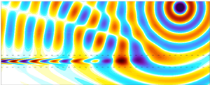Figure 3 shows two samples of adjoint Green's problem solved among a total set of $69$. Wherever the mean velocity gradient is zero, the adjoint Lilley equation behaves like a classical acoustic propagation operator. This can be observed in figure 3 and inferred from the self-adjoint property of Lilley's equation for a constant flow profile (compare (3.3) and (3.7)). Yet wherever the mean flow is sheared, the propagation problem ceases to be self-adjoint and specific features of the adjoint formulation (3.7) are expected. The wave patterns warped in the flow channel for numerical adjoint Green's function computed at $\boldsymbol {x}_m/\sigma = (25,9.0)$ and shown in figure 3 is such a phenomenon. Recall that the fields presented in figure 3 are anti-causal and focus toward the adjoint source.

Figure 3. Numerical adjoint Green's problems associated with Lilley's equation at $\boldsymbol {x}_m = (x_1,x_2)$ for the axial positions $x_1/\sigma = 0.0$, $x_1/\sigma = 25$ and $x_2/\sigma =9.0$. $(a,c)$ Adjoint Gaussian source terms ${S}^{\dagger,N}_{\boldsymbol {x}_m}$ considered to mimic an impulse forcing, and $(b,d)$ the associated adjoint fields ${p}^\dagger$ regarded as numerical adjoint Green's functions ${G}^{\dagger,N}_{\boldsymbol {x}_m}$.

To properly define adjoint Green's function ${G}^\dagger _{\boldsymbol {x}_m}$, the impulse response of the linear operator ${\mathcal {L}}^\dagger _0$ should be considered, that is ${\mathcal {L}}^\dagger _0\ {G}^\dagger _{\boldsymbol {x}_m} = \delta _{\boldsymbol {x}_m}$. For most numerical solvers, computing the solution to an exact Dirac delta function $\delta _{\boldsymbol {x}_m}$ is tricky. A bypass to this is considered here; narrow Gaussian sources are chosen to force the linear operator ${\mathcal {L}}^\dagger _0$ given in (3.7). Then when the size $L$ of the numerical adjoint source ${S}^{\dagger,N}_{\boldsymbol {x}_m}$ is small with respect to the acoustic wavelength $\lambda$, mathematical Green's function ${G}^\dagger _{\boldsymbol {x}_m}$ can be approximated with the following normalisation of numerical Green's function ${G}^{\dagger,N}_{\boldsymbol {x}_m}$:

(3.10)\begin{equation} {G}^\dagger_{\boldsymbol{x}_m}(\boldsymbol{x}) \approx {G}^{\dagger,N}_{\boldsymbol{x}_m}(\boldsymbol{x})\left/ \displaystyle \int_\Omega {{S}^{\dagger,N}_{\boldsymbol{x}_m}}^*(\boldsymbol{y}) \,\textrm{d}\boldsymbol{y}\right., \end{equation}

where ${S}^{\dagger,N}_{\boldsymbol {x}_m}$ is the numerical source term of the adjoint problem, chosen presently to be a sharp Gaussian around ${\boldsymbol {x}_m}$. For a Gaussian source, its size $L$ is measured by its standard deviation $\sigma _{s}$, for the present analysis, $\lambda /\sigma _{s}\approx 23$. Following this procedure, for each adjoint solution, adjoint Green's function ${G}^\dagger _{\boldsymbol {x}_m}$ is defined. Lagrange's identity (2.2) then readily gives at each sample position $\boldsymbol {x}_m$ the physical pressure field $p(\boldsymbol {x}_m)$:

(3.11)\begin{equation} p(\boldsymbol{x}_m) = \left\langle {G}^\dagger_{\boldsymbol{x}_m},S_{Lilley}\right\rangle = \displaystyle \int_\Omega {{G}^\dagger}^*_{\boldsymbol{x}_m}(\boldsymbol{x})\ S_{Lilley}(\boldsymbol{x})\,\textrm{d}\boldsymbol{x}. \end{equation}

Results obtained for the investigated sampled line are compared in figure 4 against the direct problem solution seen as a reference. Figure 4 shows an almost perfect reconstruction of the reference field with the adjoint method, demonstrating thus the viability of the approach, and gives an a posteriori validation of the utilised numerical trick to compute an anti-causal solution (refer to appendix B.). In practice, the only limitation of the method is the ability to properly compute numerical adjoint Green's function. The bypass procedure, given in (3.10), requiring that the adjoint source is compact ($\lambda /L\gg 1$) proves to work correctly as well.

Figure 4. Validation of the adjoint method along the line $x_2/\sigma = 9.0$ for Lilley's equation. Reference data for the pressure $p$ (real part, ——; imaginary part, - - - -) is taken from the direct field computation presented in figure 2. Rebuilt pressure field $p$ (real part, $\circ$; imaginary part, $+$) is obtained with Lagrange's identity.

3.4. Reconstruction of the solution with the FRT

The FRT introduced by Lyamshev (Reference Lyamshev1961) and Howe (Reference Howe1975), and formulated in a more general statement by Godin (Reference Godin1997), exploits alternatively the reciprocity principle to rebuild the physical field. The FRT is used here and applied to Lilley's wave equation to enable comparison with the adjoint method.

In the framework of the FRT, the reciprocal problem is obtained from the direct one (2.1) by turning the velocity dependences in $\boldsymbol {u}_0$ in the linear operators $\mathcal {L}_0$ and $\mathcal {B}_0$ into $-\boldsymbol {u}_0$. The corresponding operators will be referred to as $\mathcal {L}^-_0$ and $\mathcal {B}^-_0$, the reciprocal field $p^-$ is then governed by the FRT equations

(3.12)\begin{equation} \begin{cases} \mathcal{L}^-_0\ p^- = s^- & \text{in} \ \Omega\\ \mathcal{B}^-_0\ p^- = 0 & \text{on} \ \partial\Omega \end{cases}, \end{equation}

where $s^-$ is the source for the FRT problem considered. In practice, it is sufficient to invert the mean flow $\boldsymbol {u}_0$ direction in the direct problem solver to compute $p^-$. This has been achieved for Lilley's wave equation for which simulations are conducted for the same sampling of sources as for the adjoint problem presented in the previous paragraph, that is by taking $s^- \equiv {s}^\dagger$. The same mean density $\rho _0$, pulsation frequency $\omega$ and mesh as for the direct problem are considered. Again, Green's solutions to $\mathcal {L}^-_0$ are considered and (3.4) is therefore discarded. Some realisations for the reciprocal field $p^-$ for different sample locations are shown in figure 5.

Figure 5. Numerical FRT Green's problems associated with Lilley's equation at $\boldsymbol {x}_m = (x_1,x_2)$ for the axial positions $x_1/\sigma = 0.0$, $x_1/\sigma = 25$ and $x_2/\sigma =9.0$. $(a,c)$ Gaussian source terms $S^{-,N}_{\boldsymbol {x}_m}$ considered to mimic an impulse forcing and $(b,d)$ the associated reciprocal fields $p^-$ regarded as numerical FRT Green's functions $G^{-,N}_{\boldsymbol {x}_m}$. The same range for the colourmaps as in figure 3 is used.

A normalisation procedure similar to (3.10) is used to compute FRT reciprocal Green's function $G^-_{\boldsymbol {x}_m}$ from the numerical FRT field $G^{-,N}_{\boldsymbol {x}_m}$. In a similar fashion to (2.2), the pressure field $p$ solution of the direct problem is rebuilt with

(3.13)\begin{equation} p(\boldsymbol{x}_m) = \left\langle G^-_{\boldsymbol{x}_m},S_{Lilley}\right\rangle_{\mathbb{R}}, \end{equation}

where the scalar product for real-valued functions $\langle, \rangle _{\mathbb {R}}$ should be used, according to Lyamshev (Reference Lyamshev1961, equation (14)), defined for the functions $f$ and $g$ by

(3.14)\begin{equation} \langle \, f,g\rangle_{\mathbb{R}} = \int_{\Omega} \,\textrm{d}\boldsymbol{x}\ f(\boldsymbol{x}) g(\boldsymbol{x}). \end{equation}

The explanation why a non-Hermitian scalar product is needed in the application of the FRT is discussed later in § 4.3. The pressure field $p$ obtained along the sampled line with the FRT is compared in figure 6 against the direct problem solution taken as reference.

Figure 6. Validation of the FRT method along the line $x_2/\sigma = 9.0$ for Lilley's equation. Reference data for the pressure $p$ (real part, ——; imaginary part, - - - -) is taken from the direct field computation presented in figure 2. Rebuilt pressure field $p$ (real part, $\circ$; imaginary part, $+$) is obtained with(3.13).

In this example, the FRT recovers very poorly the direct problem solution both qualitatively as quantitatively. In this configuration a relative error greater than $300\,\%$ is observed at some observer locations, this error grows when the considered pulsation frequency $\omega$ decreases. A comparative look at the reciprocal fields obtained with the FRT, in figure 5, and with the adjoint method, in figure 3, reveals striking differences in both computed reciprocal fields. Subtle phenomena seem indeed to occur in the region of flow gradients in the adjoint approach which are not described by the FRT methodology; note that this region coincides with the region for which $\mathcal {L}_0$ is not self-adjoint. Furthermore this region of flow gradient is precisely where the source $S_{Lilley}$ for the direct problem is located and, according to (3.11) and (3.13), it is the part of the reciprocal fields that contributes to the value of the rebuilt pressure $p$ at the sample locations $\boldsymbol {x}_m$. This paragraph highlights hence, that the rigorous computation of an acoustic field over a shear mean flow is typically a case for which the commonly used reciprocity principle – even if extended with the FRT – fails and where the general adjoint framework is required.

4.1. Solution to the direct problem

The direct problem under consideration is made of Pierce's wave equation completed with some radiating boundary conditions $\mathcal {B}_0$

(4.2)\begin{equation} \begin{cases} \mathcal{L}_0\ \phi = D_{\boldsymbol{u}_0}^2(\phi) - \boldsymbol{\nabla} \boldsymbol{\cdot} ( a_0^2 \boldsymbol{\nabla} \phi) = S_{Pierce} & \text{in} \ \Omega,\\ \mathcal{B}_0\ \phi = 0 & \text{on} \ \partial\Omega, \end{cases} \end{equation}

where $S_{Pierce}$ is built according to (4.1) and is based on the same LEE equivalent source terms $(S_{\rho },\boldsymbol {S}_{\boldsymbol {u}},S_p)$ as used for $S_{Lilley}$. For simplicity, the quadrupole source $\rho _0 \boldsymbol {S}_{\boldsymbol {u}}$ considered in § 3.2 was chosen in this study to derive from a potential source $S_m$. For arbitrary sources, a filtering process based on a Poisson solver has proved to give very satisfactory results for Pierce's equation when compared with the solution for the unfiltered source computed with Lilley's equation. The computation of $\phi$ described in Pierce's direct problem (4.2) is achieved with the in-house code PROPA. The same mean flow field and the same frequency are analysed as previously for Lilley's wave equation. The fluctuating pressure $p$ is then straightforwardly rebuilt with $p = - D_{\boldsymbol {u}_0}(\phi )$ and is shown in figure 7.

Figure 7. Direct problem for Pierce's wave equation. $(a)$ Source for Pierce's potential acoustic wave equation $S_m$ equivalent to the quadrupole $\rho _0 \boldsymbol {S}_{\boldsymbol {u}} (= \boldsymbol {\nabla } S_m)$ shown in figure 2. $(b,c)$ Mach number $M_0$ and density $\rho _0$ profiles of the parallel mean flow considered and the real part of the pressure field $p = -D_{\boldsymbol {u}_0}(\phi )$ is shown with the same range for the colourmap as in figure 2. Dashed lines represent the position of maximal shearing ($x_2/\sigma = 1$).

4.2. Reconstruction of the solution with the adjoint method

Repeating the procedure given in § 3.3, the adjoint method is used here to recover the velocity potential $\phi$ associated with the direct field. The fluctuating pressure $p$ is rebuilt subsequently. The same sampling of adjoint sources used previously, partly shown in figure 3, is considered here. Each of these adjoint sources is defined as a sink term to the anti-causal adjoint Pierce problem

(4.3)\begin{equation} \begin{cases} {\mathcal{L}}^\dagger_0\ {\phi}^\dagger = D_{\boldsymbol{u}_0}^2({\phi}^\dagger) - \boldsymbol{\nabla} \boldsymbol{\cdot} ( a_0^2 \boldsymbol{\nabla} {\phi}^\dagger) & \text{in}\ \Omega,\\ {\mathcal{B}}^\dagger_0\ {\phi}^\dagger = 0 & \text{on}\ \partial\Omega. \end{cases} \end{equation}

Because Pierce's wave equation is self-adjoint for the scalar product (3.2) chosen here, its associated adjoint problem is nothing other than Pierce's wave equation completed with some anti-radiating boundary conditions ${\mathcal {B}}^\dagger _0$. The same features for the mean flow and the numerical settings as for previous calculations are considered. Figure 8 shows the adjoint velocity potential fields ${\phi }^\dagger$ solution to Pierce's adjoint problem taken at two sample locations.

Figure 8. Numerical adjoint Green's problems associated with Pierce's equation at $\boldsymbol {x}_m = (x_1,x_2)$ for the axial positions $x_1/\sigma = 0.0$, $x_1/\sigma = 25$ and $x_2/\sigma =9.0$. $(a,c)$ adjoint Gaussian source terms ${S}^{\dagger,N}_{\boldsymbol {x}_m}$ considered to mimic an impulse forcing and $(b,d)$ the associated adjoint fields ${\phi }^\dagger$ regarded as numerical adjoint Green's functions ${G}^{\dagger,N}_{\boldsymbol {x}_m}$. The range for the colourmaps used here differs from the one used in figures 3 and 5.

As previously, adjoint Green's functions ${G}^\dagger _{\boldsymbol {x}_m}$ are computed from previous numerical adjoint functions ${G}^{\dagger,N}_{\boldsymbol {x}_m}$ using the compacity assumption of the adjoint source. Lagrange's identity then gives straightforwardly at each sample position $\boldsymbol {x}_m$,

(4.4)\begin{equation} \phi(\boldsymbol{x}_m) = \left\langle {G}^\dagger_{\boldsymbol{x}_m},S_{Pierce}\right\rangle, \end{equation}

and subsequently the acoustic pressure $p = - D_{\boldsymbol {u}_0}(\phi )$. Results obtained for the fluctuating pressure $p$ along the sampled line are compared in figure 9 against Pierce's direct problem solution taken as reference.

Figure 9. Validation of the adjoint method along the line $x_2/\sigma = 9.0$ for Pierce's equation. Reference data for the pressure $p$ (real part, ——; imaginary part, - - - -) is rebuilt from the direct field computation using $p = - D_{\boldsymbol {u}_0}(\phi )$ as presented in figure 7. Similarly, the rebuilt pressure field $p$ (real part, $\circ$;imaginary part, ${+}$) is computed from the velocity potential field $\phi$ computed with Lagrange's identity. Dotted lines, $\cdots \cdots$, display the corresponding real and imaginary parts of the pressure $p$ solution to Lilley's equation given in figure 4.

Again in figure 9, an almost perfect reconstruction of the reference pressure field $p$ is obtained with the adjoint method. On an indicative basis, figure 9 also shows the pressure field $p$ computed previously with Lilley's wave equation. The satisfactory ability of Pierce's wave equation to compute acoustic refraction effects for the high-speed heated sheared mean flow encountered here is enlightening. This potential acoustic prediction is all the more satisfactory, since Pierce's equation is known to be accurate in the high-frequency limit (Pierce Reference Pierce1990), which is not fulfilled here, $\lambda / \sigma \approx 3$.

4.3. The adjoint method and the FRT equivalence for self-adjoint operators

In this study on Pierce's wave equation, the field reconstruction achieved with the FRT is not shown. Rigorously the same results as those presented for the adjoint method in figures 8 and 9 would have indeed been obtained. This is because the adjoint method and the FRT are fully equivalent for self-adjoint operators. A proof for this is given here for Helmholtz's wave equation written for a uniform steady background flow. Three-dimensional Green's function for the latter is recalled in appendix B. and solutions to the direct and adjoint propagation problems can be expressed as

(4.5)\begin{equation} G_{\boldsymbol{x}_s}(\boldsymbol{x},\omega) = \exp\left( -\textrm{i} \dfrac{\omega}{a_0} \dfrac{ \boldsymbol{M}_0 \boldsymbol{\cdot} (\boldsymbol{x}-\boldsymbol{x}_s) }{1-M_0^2} \right) \dfrac{\exp\left( \textrm{i} \dfrac{1}{1-M_0^2} \dfrac{\omega}{a_0} r_{\boldsymbol{x}_s} \right) }{4{\rm \pi} r_{\boldsymbol{x}_s}} \end{equation}

and

(4.6)\begin{equation} {G}^\dagger_{\boldsymbol{x}_m}(\boldsymbol{x},\omega) = \exp\left( -\textrm{i} \dfrac{\omega}{a_0} \dfrac{ \boldsymbol{M}_0 \boldsymbol{\cdot} (\boldsymbol{x}-\boldsymbol{x}_m) }{1-M_0^2} \right) \dfrac{\exp\left( -\textrm{i} \dfrac{1}{1-M_0^2} \dfrac{\omega}{a_0} r_{\boldsymbol{x}_m} \right) }{4{\rm \pi} r_{\boldsymbol{x}_m}}, \end{equation}

where $r_{\boldsymbol {x}_i} = \sqrt {(1-M_0^2) |\boldsymbol {x} - \boldsymbol {x}_i|^2 + (\boldsymbol {M}_0 \boldsymbol{\cdot} (\boldsymbol {x}-\boldsymbol {x}_i))^2}$ and $\boldsymbol {M}_0 = \boldsymbol {u}_0/a_0$ is the vectorial Mach number. Furthermore, let $G_{\boldsymbol {x}_m}^-$ be Green's function in $\boldsymbol {x}_m$ solution of the FRT. Then $G_{\boldsymbol {x}_m}^-$ can be deduced from the expression of $G_{\boldsymbol {x}_s}$ by switching the source $\boldsymbol {x}_s$ and the observer $\boldsymbol {x}_m$ positions and reversing the mean velocity $\boldsymbol {u}_0$ direction. Consistently with what is carried out for the numerical simulations in the frequency domain, it is argued that the anti-causal solution for the adjoint problem ${G}^\dagger _{\boldsymbol {x}_m}$ can be selected considering the usual radiating solution, but for an opposite pulsation frequency $\omega$. From the above obtained analytical expressions, the equivalence of the reciprocal fields computed with the adjoint method or the FRT are then easily verified:

(4.7)\begin{equation} {G}^\dagger_{\boldsymbol{x}_m}(\boldsymbol{x},\omega) = G_{\boldsymbol{x}_m}^-(\boldsymbol{x},-\omega). \end{equation}

Since analytical solutions to acoustic propagation problems are scarce, directly assessing this symmetry with respect to the flow reversal on general analytical solutions is hopeless. However, this symmetry in the exchange of the mean flow direction and the sign of the pulsation frequency $\omega$ of the acoustic solution can already be assessed from the linear operator $\mathcal {L}_0$ governing the wave propagation. And effectively, in Pierce's wave operator, changing the sign of $\omega$ or $\boldsymbol {u}_0$ appears to be fully equivalent. This remark holds for all self-adjoint wave equations describing acoustic propagation over a moving flow, namely the ones introduced by Galbrun (Reference Galbrun1931), Phillips (Reference Phillips1960), Goldstein (Reference Goldstein1978), Godin (Reference Godin1997) and Möhring (Reference Möhring1999).

On top of that, a critical literature review reveals that in the studies illustrating the FRT, only self-adjoint wave equations written in the frequency domain are considered. The proof for the FRT reciprocity relation, classically starts with the multiplication of the wave equation governing the direct propagation problem by a field variable, and its integration over the entire propagation domain. In fact, this operation closely resembles a scalar product multiplication with a test function or a Lagrange multiplier. Integration by parts of the direct problem wave equation then frees the direct field variable and defines the reciprocal wave equation with reversed flow to which the previously introduced test function is subject, i.e. the FRT for the considered wave equation is readily demonstrated. The difference with the adjoint method lies in the scalar product which is not well-posed for the FRT. As a matter of fact, manipulating a wave equation written in the frequency domain requires the introduction of a Hermitian scalar products. If the latter condition were fulfilled in the FRT proof, the self-adjoint property of the equation would have been retrieved and in turn no flow reversal needed. It appears now clearly why only $\mathbb {R}$ space scalar products should be considered in the final solution reconstruction with the FRT, to say,

(4.8)\begin{equation} \phi = \left\langle {G}^\dagger_{\boldsymbol{x}_m},S_{Pierce}\right\rangle = \left\langle G^-_{\boldsymbol{x}_m},S_{Pierce}\right\rangle_{\mathbb{R}}. \end{equation}

The reciprocal field $G_{\boldsymbol {x}_m}^-$ computed with the FRT is in fact, the complex conjugate of the adjoint field ${G}^\dagger _{\boldsymbol {x}_m}$. This is easily seen, taking benefit of the Fourier transform property of a real-valued field $G_{\boldsymbol {x}_m}^-(\boldsymbol {x},-\omega )={G^-}^*_{\boldsymbol {x}_m}(\boldsymbol {x},\omega )$ for which it follows from (4.7):

(4.9)\begin{equation} G_{\boldsymbol{x}_m}^-(\boldsymbol{x},\omega) = {{G}^\dagger}^*_{\boldsymbol{x}_m}(\boldsymbol{x},\omega). \end{equation}

The equivalence between the adjoint method and the FRT for self-adjoint operators has pragmatic implications. The solving of anti-causal adjoint equations can indeed be advantageously replaced by direct computations over reversed flow. An interesting question to answer is whether some linear operators may all at once describe exactly acoustic propagation over a sheared mean flow and be self-adjoint. Möhring (Reference Möhring1999) answered this question and illustrated how from a self-adjoint operator an energy-conserving law could be derived for the acoustic field. Yet, it is well known that for sheared flows, instability waves may occur converting acoustic energy into vortical energy (Yates Reference Yates1978; Maestrello, Bayliss & Turkel Reference Maestrello, Bayliss and Turkel1981) and thus that no such conservation law for acoustic energy exist. Hence for arbitrary mean flows, acoustic energy is not preserved, and a linear operator which is twofold self-adjoint and exactly describes acoustic propagation does not exist. If acoustic propagation in a complex media needs to be conducted very accurately, a non-self-adjoint operator needs therefore to be considered. Nevertheless if a decoupling of the acoustic with the vortical mode is required for stability purposes, and approximations tolerated, Pierce's wave equation seems to achieve nicely the prediction of flow refraction effects on sound.