MoM procedure with CSP type Green's function

To obtain a unidirectional CSP beam, the real source coordinate x′ of the line current type was replaced by a complex quantity [Reference Felsen4]:

(1)$$\vec {x}^{\, \prime} \to {\vec x}^{\, \prime}_{csp} = \vec {x}^{\, \prime} - j\vec b,\quad \vec b = \hat bb,$$

where b is defined as the beam aperture, while the unit vector $\hat b$ defines the direction of the beam radiation. Considering a beam that radiates from the real point x′ to the upward y-direction, if $\vec {x}^{\, \prime}$ is converted to ${\vec x}^{\, \prime}_{csp}$, then the omnidirectional cylindrical wave becomes a unidirectional beam field. To realize this in the E-polarization case, the CSP type Green's function is applied to electric field integral equation (EFIE):

(2)$$E_z^s = - jk\eta \int_0^L {J_z({x}^{\, \prime},b)G_{csp}(x - {x}^{\, \prime},b({x}^{\, \prime}))d{x}^{\, \prime}}, $$

where k is the wavenumber and η is the intrinsic impedance. Here J _z(x′, b) is the unknown current density function different from the physical current on the strip and G _csp is the CSP type Green's function that is given as:

(3)$$G_{csp}(x - {x}^{\prime},b({x}^{\prime})) = \displaystyle{{ - j} \over 4}H_0^{(2)} (k\sqrt {{(x - {x}^{\prime})}^2 - b{({x}^{\prime})}^2} ).$$

Here, b(x′) is the beam parameter, which depends on the position. It was observed that the complex line beam field normalized to the maximum value of radiation, that is |G _csp|, becomes very small if |x| > b as shown in Fig. 2(a). Therefore, there would be almost no interaction between the source and observation elements on the strip if they are far enough from each other. This provides a strong localization of the main matrix so that many of its elements are very close to zero and can be safely neglected. This converts the main matrix into a sparse one, which is an attractive achievement as there are certain algorithms to solve the sparse matrices more efficiently compared with the full matrices. As known, typically the total number of unknowns is very large in MoM that restricts its application to the analysis of electrically large geometries.

Fig. 2. (a) Normalized beam field |G _csp| versus x/λ and (b) Beam radiation field for x′ = 0, y′ = 0, and b = 1λ.

The incident field is assumed to be a plane wave, $E_z^{in} = e^{jk(x\cos \phi _{in} + y\sin \phi _{in})}$. Then, to discretize EFIE (2) to a matrix form, the unknown function is approximated by the pulse basis functions with unknown coefficients a _n’s, n = 1, 2… N (see [Reference Volakis and Sertel18] for details). Furthermore, the Galerkin MoM technique is applied to obtain the following matrix equation:

(4)$$\int_{x_m-\Delta /2}^{x_m + \Delta /2} { p_m(x)E_z^{in} (x)} dx = -jk\eta \sum\limits_{n = 1}^N {a_n\int_{x_m-\Delta /2}^{x_m + \Delta /2} { p_m(x)} } \int_{x_n-\Delta /2}^{x_n + \Delta /2} { p_n(x^{\prime})G_{csp}(x-x^{\prime},b_n)dx^{\prime}dx} .$$

Here, b _n is the complex beam parameter depending on the source indices i.e. the location of the basis function, Δ is the discretization length of the strip surface, and it is selected as λ/10 to follow the rule-of-the-thumb discretization criteria. It takes the value of zero in the near edge regions, b _n = 0, and a real constant value in the non-near edge region b _n = b, on the strip. In this procedure, the p _n(x) functions are chosen as the small pulses where x _n’s are the middle points of these pulses. The singularity extraction procedure was also performed at the branch points of the complex line source located at x = x′ + b and x = x′−b, where b is a selectable beam width parameter. The CSP beam-like field is clearly visible in Fig. 2(b).

The incident field for the H-polarization is assumed as a plane wave, $H_z^{in} = e^{jk(x\cos \phi _{in} + y\sin \phi _{in})}$. The next step is to apply the Galerkin method with triangular basis functions t _n(x). The current density is again expanded with the unknown coefficients, a _n’s, n = 1,2…N−1 to generate the following matrix equation:

(5)$$\eqalign{ \int_{x_m-\Delta }^{x_m + \Delta } {t_m(x)E_x^{in} (x)dx = &-jk\eta \sum\limits_{n = 1}^{N-1} {a_n\int_{x_m-\Delta }^{x_m + \Delta } {t_m(x)} } \int_{x_n-\Delta }^{x_n + \Delta } {t_n(x^{\prime})} G_{csp}(x-x^{\prime},b_n)dx^{\prime}dx} \cr & + \displaystyle{{ j\eta } \over k}\sum\limits_{n = 1}^{N-1} {a_n} \int_{x_m-\Delta }^{x_m + \Delta } {\displaystyle{{\partial t_m(x)} \over {\partial x}}} \int_{x_m-\Delta }^{x_m + \Delta } {\displaystyle{{\partial t_n(x^{\prime})} \over {\partial x^{\prime}}}} G_{csp}(x-x^{\prime},b_n)dx^{\prime}dx.} $$

It is possible to express equations (4) and (5) in the matrix form, $\lsqb {Z_{mn}^{E,H}} \rsqb \lsqb {a_n} \rsqb = \lsqb {W_m^{E,H}} \rsqb $, where $Z_{mn}^{E,H} $ is the main matrix and $W_m^{E,H} $ is the discretized left-hand part of the integral equation in either polarization.

Main concept of the method and determination of the parameters “b” and “α”

The CSP field is a beam in free space and it is the exact solution of the Helmholtz equation, additionally satisfying the radiation condition. The PEC boundary condition on the strip was used in the formulation of the problem. To keep the edge condition intact, the free space Green's function was adjusted by setting the b parameter as zero in the vicinity of the edge. The distance parameter α is as large as possible to prevent the radiation of the surface current on the edges.

The rough view of the main matrix filled with numbers is a pattern in Figs 3(a) and 3(b) for L = 10λ. The standard MoM in the E-pol case produces a dense matrix (see Fig. 3(a)) but as shown in Fig. 3(b), with our technique, the main impedance matrix is converted to a sparse form indicated by white parts in the mapping as almost zero magnitude.

Fig. 3. The magnitude level of the impedance matrix elements for L = 10λ, Δ = 0.1λ (a) standard MoM and (b) the proposed method for E-pol with α = 2λ and b = 1λ, (c) standard MoM, and (d) the proposed method for H-pol with α = 2λ and b = 1.3λ (Green dashed lines marked for explanation).

In the H-pol case, two integrals of the main matrix were studied standing in the right-hand part of (5). The main impedance matrix is converted to a sparse form just like in E-pol and the patterns of the main matrix elements are shown in Figs 3(c) and 3(d). Due to these remarkable features, the proposed hybrid technique provides an important advantage in computer storage and calculation time.

The CSP Green's function (G _csp) tends to zero in the region of x ≥ 1 as shown in Fig. 2(a). The function has a numerical value only in the region of x < 1, however, it is almost zero if x ≥ 1. It is expected that “α” should be greater than “b” so that the near edge region is not illuminated by complex source radiation of the basis functions on the strip surface. Due to this selection, the edges do not enter the beam apertures on the scatterer surface and the edge condition is unaltered and preserved.

Then, the main matrix elements are used to find the radiated electric field as an explanation of the interactions. For n = 1, the matrix column Z _m1 is linked to the interval between “m” and “1”. This interval does not depend on the location of the basis function due to the fact that the Toeplitz matrix has a hierarchy of shift-invariant. Here, what is important is the difference between “m” and “1”, which describes the distance between the source location and the testing location. This column matrix indicating the radiated electric field presents a reduction with the distance away from the source. Therefore, the basis function (as indicated, n = 1) can be selected for any source location in the non-near edge region where b ≠ 0. The goal is to observe the behavior of the complex source beam radiation in the non-near edge region. Hence, called Z _ms, where “s” is a static index (basis function index only for CSP in the non near-edge region) indicating the CSP location, and “m” is a non-static index number (testing function index) that indicates the location of testing function; it varies from 1 to N in E-pol and to N−1 in H-pol. For any CSP in the non-near edge region, it means whatever “s” is assigned, the behavior of the CSP beam radiation is identical for any specific “b”. Accordingly, the index “s” is assigned to any CSP location and the matrix Z _ms degradated to Q _|m−s| in order to observe just one CSP. In brief, Q _|m−s| is the testing vector of any CSP in the non-near edge region, that is, it is a column matrix of Z _ms corresponding to any number of “s”. For instance, in Figs 3(b) and 3(d), since α = 2λ, “s” index varies from 20 to 80 for the case of the total number of unknown N = 100 and Δ = 0.1λ. In this case, the main matrix is not a good sparse matrix, the parameters α, b, L have been specified so that the figure is easily visible and the band structure shows non-zero matrix elements. Q _|m−s| column matrices form the band structure in that region, for example, in Fig. 3(b), if “s” or “n” index is 50, since b = 1λ, “m” index takes any value from 40 to 60 and these values indicate two identical column vectors. Each side is symmetrical and has a pattern like G _csp in terms of magnitude (see Fig. 2(a)). In this column matrix, the maximum value for each side is at m = 50 and minimum values are at m = 40 and m = 60 for this example. For the sake of simplicity, we viewed the one side |Q _|m−s|| as shown in Fig. 4. As stated above, Q _|m−s| column matrices are identical for any index number of “s” in the band structure, so |Q _|m−s|| was investigated independently from the “s” index.

Fig. 4. Normalized function |Q _|m−s|| versus x/λΔ at x′ = 0 (a) E-polarization, (b) H-polarization.

We implemented the approximation Z _ms = 0 for the regions where “|m −s|” distance is greater than “b” as shown in Figs 3(b) and 3(d). Therefore, analyzing the normalized function |Q _|m−s|| versus the “|m −s|” index difference is a worthy intention. The parts where “|m −s|” distance is greater than “b” provide an insight into the approximation. These concepts depending on Z_mn can be applied to the other 2D geometries for determination of α and b.

Resulting |Q _|m−s|| varies depending on the polarization, as shown for E-pol and H-pol in Figs 4(a) and 4(b). A descending pattern of |Q _|m−s|| in H-pol was observed more widely compared with the E-pol. Also, the decrease of |Q _|m−s|| is smaller in H-pol than in E-pol for any value of “b”. Thus, selecting larger “b” in H-pol is a necessity so that the approximated parts are closer to zero.

Typically, b = 1λ can be assigned for both polarizations whose relative errors are <1% as shown in the numerical results. However, for more accurate results, b > 1λ can be assigned. There is a trade-off, because the selection of “b” affects the computing and filling the main matrix, hence the computational time. Taking a larger value of “b” means decreasing the sparsity of the main matrix. Experiments show that |Q _|m−s|| at “|m−s|” should be less than 10⁻³, corresponding to b = 1.5λ and b = 2λ for E-pol and H-pol, respectively.

It is not important to select “α” in the scale of larger values than “b” and α > b can be assigned. Nonetheless, larger “α” values ensure the correction in the minor lobes, especially in the angles close to 0° and 180° in RCS. These corrections are not significant compared with the main lobe since they are negative in the dB scale of RCS.

In the light of the findings described above, at the normal incidence, b = 1.5λ and α = 2.5λ were assigned in E-pol, b = 2λ and α = 3λ in H-pol, to properly represent the method. At the inclined incidence, since the edges are less effected by the radiation of CSP and the edges are more important, the near edge regions must be wider. Namely, “α” is assigned larger values, for example, b = 1.5λ and α = 4λ were assigned for E-pol, b = 2λ, and α = 4λ for H-pol at the inclined incidence, ϕ ⁱⁿ = 30°. Taking a larger value of α extends the near edge regions so that the method is more dominant at the grazing incidence illumination.

Determination of the radiation characteristics

After the numerical solution of the matrix equation (4), one obtains the current density which is not the real current density of the original problem. However, the convolution of this current with G _csp can then produce the true scattered pattern. The far zone electric field scattered from the strip can be written as:

(6)$$\!\!\!\eqalign{E_z^{sc} = \sqrt {\displaystyle{2 \over {\,j\pi kr}}} \cdot e^{ - jkr}\underbrace{{( - k\eta /4)\sum\limits_{n = 1}^N {a_n} e^{kb_n\sin \phi} \int\limits_{x_n - 0.5\Delta} ^{x_n + 0.5\Delta} {\,p_n({x}^{\prime})} e^{\,jk{x}^{\prime}\cos \phi} d{x}^{\prime}}}_{{\psi ^1(\phi )} } }{\vskip1pc,}$$

where ψ ¹(ϕ) is the scattering pattern and ϕ is the observation angle. The monostatic RCS can be given as:

(7)$$\sigma = 2\pi r\displaystyle{{{\vert {E_z^{sc}} \vert } ^2} \over {{\vert {E_z^{in}} \vert } ^2}} = \displaystyle{4 \over k}\vert {\psi^1(\phi )} \vert ^2$$

Similarly, the current function is obtained from (5) for H-pol and the far zone magnetic field scattered from the strip can be written as:

(8)$$\eqalign{H_z^{sc} = \sqrt {\displaystyle{2 \over {\,j\pi kr}}} \cdot e^{ - jkr}\underbrace{{(k/4)\sin \phi \sum\limits_{n = 1}^{N - 1} {a_n} e^{kb_n\sin \phi} \int\limits_{x_n - \Delta} ^{x_n + \Delta} {t_n({x}^{\prime})} e^{\,jk{x}^{\prime}\cos \phi} d{x}^{\prime}}}_{{\psi ^2(\phi )}}.$$

Then, the true scattered pattern can be found by using this current function, which is not the real one in the convolution with G _csp and the monostatic RCS is given as:

(9)$$\sigma = 2\pi r\displaystyle{{{\vert {H_z^{sc}} \vert } ^2} \over {{\vert {H_z^{in}} \vert } ^2}} = \displaystyle{4 \over k}\vert {\psi^2(\phi )} \vert ^2.$$

MoM procedure with CSP type Green's function

This section considered the cylinder geometry with four edges as shown in Fig. 5.

The same procedure as for the strip geometry (see the section “2D scattering from a large PEC strip”) is followed with:

(10)$$\vec {r}^{\; \prime} \to \vec {r}^{\; \prime}_{csp} = \vec {r}^{\; \prime} - j\vec b\quad \vec b = \hat xb\sin (\phi ) - \hat yb\cos (\phi ),$$

where $\vec {r}^{\; \prime} = \hat x{x}^{ \prime} + \hat y{y}^{\prime}$, ϕ is the angle between the edge and the x-axis and the beam vector $ \vec {\it b}$ is directed outward from the structure for all facets. Then, the scattered field in E-pol can be presented as:

(11)$$E_z^s = - jk\eta \int_C {J_z(\vec {r}^{\, \prime},b)G_{csp}(\vec r - \vec {r}^{\, \prime},b(\vec {r}^{\, \prime}))d\vec {r}^{\, \prime}}, $$

where C is the counter-clockwise path of the cross-sectional contour. The CSP type Green's function for this geometry is described as:

(12)$$\eqalign{G_{csp}(\vec r - \vec r^{\, \prime},b(\vec r^{\, \prime})) = - \displaystyle{\,j \over 4}H_0^{(2)} \left( {k\sqrt {{({\tilde x}_m - \tilde x_{csp}^{\, \prime} )}^2 + {({\tilde y}_m - \tilde y_{csp}^{\, \prime} )}^2}} \right)\quad \cr \quad m,n = 1,2, \ldots, N,$$

where $\tilde {x}^{\prime}_{csp} = \tilde {x}^{\prime}_n - jb_n\sin ({\phi} ^{\prime}_n)$ and ${\tilde y}^{\prime}_{csp} = {\tilde y}^{\prime}_n + jb_n\cos ({\phi} ^{\prime}_n)$, also the rectangular coordinate parameters are defined below as:

(13a)$$(\tilde x_m,\tilde y_m) = \lpar {x_{ms} + \ell \cos (\phi_m),y_{ms} + \ell \sin (\phi_m)} \rpar ,$$

(13b)$$(\tilde {x}^{\prime}_n,\tilde {y}^{\prime}_n) = \lpar {{{x}^{\prime}}_{\!\! ns} + {\ell}^{\prime}\cos ({{\phi}^{\prime}}_{\!\! n} ),{{y}^{\prime}}_{\! \! ns} + {\ell}^{\prime}\sin ({{\phi}^{\prime}}_{\! \! n})} \rpar .$$

This is a coordinate transformation from $(\tilde x_m,\tilde y_m)$ to (ℓ, ϕ _m) on m’th testing function, x _ms and y _ms are the initial coordinates of the m’th pulse testing function, ℓ is the variable along the path in the used coordinates as visible in Fig. 6(a). Then, the integral limits are adjusted according to these coordinates along the contour. For the basis functions, the format is the same as in Galerkin's procedure.

Fig. 6. Testing functions (a) pulse function for E-pol and (b) triangular function for H-pol.

Similar to the strip scattering, b _n is the complex beam parameter. We select b _n = 0 in the near edge regions and a real constant value in the non-near edge region, b _n = b. In the case of b ≠ 0, it should be noted that the beam type radiation of the basis functions interacts the testing points only on the same facet because the beam radiates outward from the facet. After some mathematical operations on the G_csp based on ${\phi} ^{\prime}_m = {\phi} ^{\prime}_n$, and application of Galerkin's procedure with pulse basis functions, the following matrix equation can be found for E-pol:

(14)$$\eqalignb{\int_0^{\Delta _m} {\,p_m(\ell ) \cdot E_z^{in} (\ell )d\ell} = - jk\eta \sum\limits_{n = 1}^N {a_n } \cr \quad \int_0^{\Delta _m} {\,p_m(\ell ) } \int_0^{\Delta _n} {\,p_n({\ell} ^{\prime})G_{csp}({\tilde x}_m - {\tilde {x}^{\prime}}_{\!\! n},{\tilde y}_m - {\tilde {y}^{\prime}}_{\!\! n},b_n)d{\ell} ^{\prime}d\ell}}}, \quad m = 1,2,3 \ldots. N,$$

where $E_z^{in} (\ell ) = e^{jk({\tilde x}_m\cos \phi ^{_{in}} + {\tilde y}_ m\sin \phi ^{_{in}} )}$ and $G_{csp}(\tilde x_m - \tilde {x}^{\prime}_n, \tilde y_m - \tilde {y}^{\prime}_n,b_n) = &InLnBrk;( - j/4)H_0^{(2)} \big( {k \scale85% \sqrt \scale110%{{({\tilde x}_m - {\tilde {x}^{\prime}}\! _n)}^2 + {({\tilde y}_m - {\tilde {y}^{\prime}} \! _n)}^2 - b_n^2}} \big)$.

In H-pol, it is applied with the triangular basis functions as depicted in Fig. 6(b). If the basis function is on the corner of the structure, the delta distance is different in each segment. Hence $\Delta _m^ - $ and $\Delta _m^ + $ are defined as the distance for the left segment and the right segment of the triangular testing function, respectively. In H-pol, CSP type Green's function is again given with a similar coordinate transformation defined on m’th testing function below:

(15a)$$(\bar x_m,\bar y_m) = \lpar {x_{m - 1} + \ell \cos (\phi_m^ - ),y_{m - 1} + \ell \sin (\phi_m^ - )} \rpar $$

(15b)$$(\bar x_m,\bar y_m) = \lpar {x_m + \ell \cos (\phi_m^ + ),y_m + \ell \sin (\phi_m^ + )} \rpar ,$$

where equation (15a) is the left segment of the triangular testing function and equation (15b) for the right segment of the triangular testing function. Besides, x _m−1, y _m−1, x _m, y _m are some related coordinates shown in Fig. 6(b), $\phi _m^ - $ and $\phi _m^ + $ are the angles between the edge and the x-axis for the left segment and the right segment of the related testing function on a facet. Note that $\phi _m^ - $ and $\phi _m^ + $ are different, if and only if, the testing function is on the corner of the structure. For the source basis functions, the format is the same. By using integration by parts, we obtain:

(16)$$\eqalignb{\int_0^{\Delta _m^ - + \Delta _m^ +} {t_m(\ell )({\hat \ell} _m \cdot {\vec E}_\ell ^{\,in} (\ell ))} d\ell &= - jk\sum\limits_{n = 1}^N {a_n} \int_0^{\Delta _m^ - + \Delta _m^ +} {\int_0^{\Delta _n^ - + \Delta _n^ +} } {({\hat \ell} _m \cdot {{\hat \ell} ^{\prime}}_n)t_m(\ell )t_n({\ell} ^{\prime})G_{csp}({\bar x}_m - {\bar {x}^{\prime}}_{\!\! n},{\bar y}_m - {\bar {y}^{\prime}}_{\!\! n},b({\ell} ^{\prime}))d{\ell} ^{\prime}}d \ell \cr & \quad + \displaystyle{\,j \over k} \sum\limits_{n = 1}^N {a_n} \int_0^{\Delta _m^ - + \Delta _m^ +} \displaystyle{\partial t_m(\ell ) \over {\partial \ell}} \int_0^{\Delta _{ n}^ - + \Delta _n^ +} \displaystyle{{\partial t_n({\ell} ^{\prime})} \over {\partial {\ell} ^{\prime}}} G_{csp}({\bar x}_m - {\bar {x}^{\prime}}_{\!\!n}, {\bar y}_m - {\bar {y}^{\prime}}_{\!\! n}, b({\ell} ^{\prime}))d{\ell} ^{\prime}d\ell \cr & \quad \quad m = 1,2,3 \ldots. N,} $$

Here $\vec E_\ell ^{in} (\ell ) = (\sin \phi ^{in}\hat x - \cos \phi ^{in}\hat y)e^{jk({\bar x}_m\cos \phi ^{_{in}} + {\bar y}_m\sin \phi ^{_{in}} )}$ and $\hat \ell _m = &InLnBrk;\hat x\cos (\phi _m) + \hat y\sin (\phi _m)$, ${\hat \ell} ^{\prime}_n = \hat x\cos ({\phi} ^{\prime}_n) + \hat y\sin ({\phi} ^{\prime}_n)$. The above equations (14) and (16) can be written in the matrix form similar to the strip geometry case, $\lsqb {Z_{mn}^{E,H}} \rsqb [a_n] = \lsqb {W_m^{E,H}} \rsqb $, where $Z_{mn}^{E,H} $ is the main matrix and $W_m^{E,H} $ is the discretized left-hand part of the integral equation, in either polarization.

Determination of the radiation characteristics

After finding the current density function of the method, in E-pol, the far zone scattered electric field from the cylinder can be written as:

(17)$$\eqalign{E_z^{sc} = \sqrt {\displaystyle{2 \over {\,j\pi kr}}} \cdot e^{ - jkr} \cr \underbrace{{( - k\eta /4)\sum\limits_{n = 1}^N {a_n} e^{kb_n\sin ({{\phi} ^{\prime}}_n - \phi )}\int_0^{\Delta _n} {\,p_n({\ell} ^{\prime})} e^{\,jk({\tilde {x}^{\prime}}_n\cos \phi + {\tilde {y}^{\prime}}_n\sin \phi )}d{\ell} ^{\prime}}}_{{\psi ^3(\phi )}},$$

where ψ ³(ϕ) is the scattering pattern. The monostatic RCS is given as:

(18)$$\sigma = 2\pi r\displaystyle{{{\vert {E_z^{sc}} \vert } ^2} \over {{\vert {E_z^{in}} \vert } ^2}} = \displaystyle{4 \over k}\vert {\psi^3(\phi )} \vert ^2.$$

In H-pol, the far zone scattered magnetic field from the cylinder is:

(19)$$\eqalign{H_z^{sc} = \sqrt {\displaystyle{2 \over {\,j\pi kr}}} \cdot e^{ - jkr} \underbrace{{( - k/4)\sum\limits_{n = 1}^N {a_n} e^{kb_n\sin ({{\phi} ^{\prime}}_n - \phi )} \int_0^{\Delta _n^ - + \Delta _n^ +} {t_n({\ell} ^{\prime})} \sin ({{\phi} ^{\prime}}_n - \phi )e^{\,jk({\bar {x}^{\prime}}_n\cos \phi + {\bar {y}^{\prime}}_n\sin \phi )}d{\ell} ^{\prime}}}_{{\psi ^4(\phi )}}.$$

The monostatic RCS is given as:

(20)$$\sigma = 2\pi r\displaystyle{{{\vert {H_z^{sc}} \vert } ^2} \over {{\vert {H_z^{in}} \vert } ^2}} = \displaystyle{4 \over k}\vert {\psi^4(\phi )} \vert ^2.$$

PEC strip geometry

In Fig. 7, the true surface current density and the current density function obtained from the proposed procedure are shown on the same plot for both polarizations. As expected, the edge effects look similar. In Fig. 8, the monostatic RCS is demonstrated for both polarizations and L = 50λ strip width.

Fig. 7. The blue line is the real current density obtained from the standard MoM, the red line is the pseudo-current function from the proposed method for the PEC 2-D strip of width L = 10λ and ϕⁱⁿ = 90°, (a) E-pol and (b) H-pol.

Fig. 8. RCS pattern comparison between standard MoM and the proposed method for L = 50λ and ϕⁱⁿ = 90°, (a) E-pol: b = 1.5λ, α = 2.5λ and RE = 0.18% and (b) H-pol: b = 2λ, α = 3λ and RE = 0.09%.

We also computed the relative error (RE) of computations, defined as:

(21)$$\bar \varepsilon = \sqrt {\sum\limits_{n = 1}^N {{\vert {e^{mom} - e^{csp}} \vert } ^2}} \left( {\sqrt {\sum\limits_{n = 1}^N {{\vert {e^{mom}} \vert }^2}}} \right)^{ - 1}.$$

Here, e^mom is the solution obtained using the standard MoM and e^csp is the solution obtained by the proposed method. Although the strip width is large, the RCS obtained is very similar to the standard MoM, with a RE of 0.18% for E-pol case and 0.09% for H-pol. Even though the condition number of the main sparse matrix for L = 50λ is approximately 10⁶, the RE is low. This low error tolerance is obtained by using the iterative algorithms with the banded preconditioned matrix. A slight deviation occurs for the directions parallel to the strip, but this region is as important in terms of the magnitude of the field.

After verification for the normal incidence, we examined the scattering near to the grazing incidence, which produced attractive results for the incidence angle, ϕ ⁱⁿ = 30° as shown in Fig. 9. Here, larger values of α were chosen for the near grazing incidence for more accurate results at the observation angles close to 0° and 180° in the RCS analysis.

Fig. 9. RCS pattern comparison for the inclined incidence between the standard MoM and the proposed method for L = 50λ (a) E-pol: ϕⁱⁿ = 30°, b = 1.5λ, α = 4λ and RE = 0.08% and (b) H-pol: ϕⁱⁿ = 30°, b = 2λ, α = 4λ and RE = 0.15%.

The RCS data was also computed closer to the near-zone region of the flat strip (see Fig. 10), comparing the standard MoM procedure with CSP type Green's function method for L = 20λ and ϕ ⁱⁿ = 90°. We get closer to the boundaries for the distance of 15λ, plotting the RCS function near the strip by taking r = 15λ and compared it with the standard MoM. As expected, our results are in agreement with the standard MoM. We considered all conditions of the electromagnetic formulation, as a result, the computed field values are correct, even when close to the strip.

Fig. 10. Near-field RCS pattern comparison between the standard MoM and the proposed method for L = 20λ and ϕⁱⁿ = 90° (a) E-pol: r = 15λ, RE = 0.2%, b = 1.5λ and α = 2.5λ and (b) H-pol: r = 15λ, RE = 0.39%, b = 2λ and α = 3λ.

Finally, the RE plots are demonstrated in Fig. 11 for the strip geometry to analyze the effect of the choice of the parameters α and b. The strip width was established as L = 50λ for both polarizations and the RE in RCS for the incidence angles of 90° and 30° was investigated. If the edge condition is fulfilled by setting the parameter α, in other words, α > b, the RE reduces. The RE plots support our choice of α and b as explained in the previous section.

Fig. 11. RE plots for the strip geometry L = 50λ (a) E-pol ϕⁱⁿ = 90°, (b) E-pol ϕ ⁱⁿ = 30°, (c) H-pol ϕⁱⁿ = 90° and (d) H-pol ϕⁱⁿ = 30°.

PEC square cross-sectional cylinder geometry

Here, the square shape of a PEC cylinder cross section is considered with a side width of 25λ. The incidence angle is assumed as ϕ ⁱⁿ = 45° for both polarizations. Due to the chosen incidence angle, the problem can be considered similar to the inclined incidence at the PEC strip, as presented above. Therefore, the CSP Green's function parameter values were assigned b = 2.5λ and α = 4λ for both polarizations, like in the inclined incidence case for the strip geometry. In Fig. 12, the obtained monostatic RCS was plotted for both polarization cases.

Fig. 12. RCS pattern comparison between the standard MoM and the proposed method for L = 25λ (a) E-pol: ϕⁱⁿ = 45°, b = 2.5λ, α = 4λ and RE = 0.13% and (b) H-pol: ϕⁱⁿ = 45°, b = 2.5λ, α = 4λ and RE = 0.14%.

Figure 13 depicts the RE plots for the PEC square cylinder geometry. In all cases for α > b, the RE values are approximately 1% or less. As highlighted earlier, the selection of the parameters b and α is convenient with the related section.

Fig. 13. RE plots for square geometry L = 25λ (a) E-pol ϕⁱⁿ = 45° and (b) H-pol ϕⁱⁿ = 45°.

Memory storage and CPU time of solution

Memory storage is an important parameter to verify the efficiency of the proposed method. The number of the main matrix elements was calculated as follows:

(22)$$\left( {\displaystyle{\alpha \over {\lambda \Delta}} N_e} \right) \cdot N + \left( {N - \displaystyle{\alpha \over {\lambda \Delta}} N_e} \right) \cdot \displaystyle{{2b} \over {\lambda \Delta}} \approx N\left( {\displaystyle{{2b} \over {\lambda \Delta}} + \displaystyle{\alpha \over {\lambda \Delta}} N_e} \right),$$

where N _e is the number of the near-edge parts on the cross-sectional contour and is equal to two for the strip geometry.

In the left-hand part of the equation above, the first term denotes the number of elements from the near-edge regions, and the second term denotes the number of elements from the non-near edge regions.

Due to the sparse form of the main matrix, the overall CPU time reduces drastically, especially for large strip widths. If the strip size is L = 500λ, N becomes 5000 if we follow the λ/10 discretization criterion. Then in the standard MoM, the main impedance matrix size becomes 5000 × 5000. Alternatively, the main matrix size obtained is approximately 80 × 5000 for α = 2.5λ and b = 1.5λ in E-pol and for the normal incidence angle. The matrix size in H-pol for the normal incidence angle is 100 × 5000. This is an extensive gain in memory storage and operation count. The memory requirement in the usual MoM is O(N ²), while it is about O(80 × N) for E-pol and O(100 × N) for H-pol in the proposed method for the single PEC strip geometry. If the size of the problem increases, then the required memory storage increases sharply when using the MoM. Substantial improvements can be obtained in the light of this, especially for very large problem dimensions. Figure 14 shows the overall running CPU times of the computation with MoM and the presented method according to the total number of unknown N.

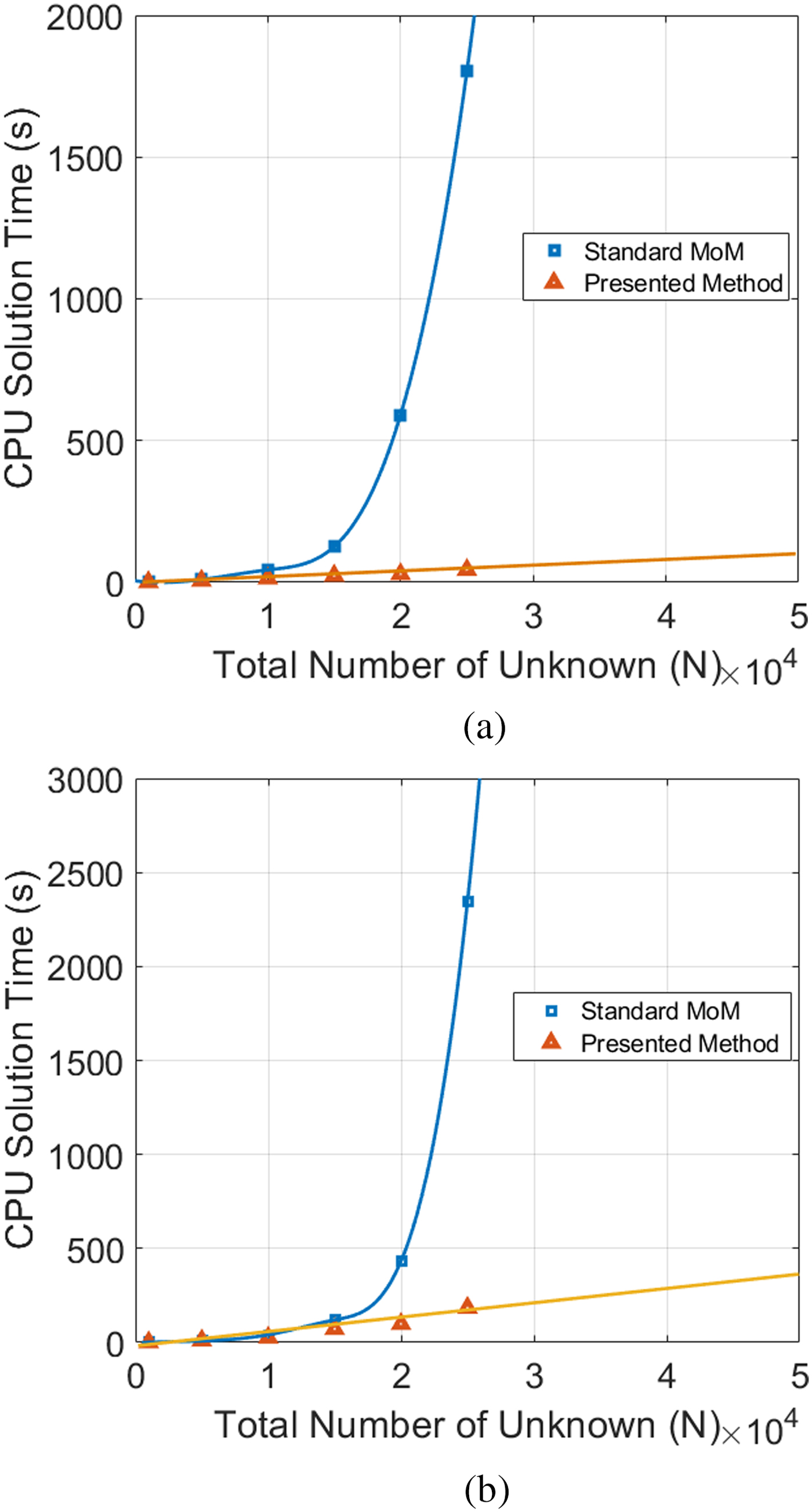
Fig. 14. The overall running CPU times of the computation versus the total number of the unknown for strip geometry (a) E-pol and (b) H-pol.

The difference in the CPU time becomes more attractive if the strip width gets larger. Beyond the total number of the unknown of 25 000 (L = 2500λ), our desktop PC does not give any results as its capacity is not enough to solve the problem with MoM, whereas the presented method can be used.

With respect to the PEC square cylinder geometry, the total size of the cross-sectional structure is 100λ and N becomes 1000 if we follow the λ/10 discretization criterion. According to equation (22), the memory requirement is O(210 × 1000) for both polarizations if α = 4λ and b = 2.5λ, while it is O(1000 × 1000) with MoM. Simultaneously obtaining a time gain of approximately 6 times and 4 times for E-pol and H-pol, respectively. Here, a larger time gain like in the strip geometry is not possible as we study the scatterer, the total size of which is 100λ (4L). This is smaller compared with the strip since the Toeplitz hierarchy does not exist for MoM and for the presented method for this geometry.