INTRODUCTION
The signature of human impacts on the environment can be detected in ice (Hong et al., Reference Hong, Candelone, Patterson and Boutron1994; Ruddiman et al., Reference Ruddiman, Fuller, Kutzbach, Tzedakis, Kaplan, Ellis, Vavrus, Roberts, Fyfe, He, Lemmen and Woodbridge2016; Uglietti et al., Reference Uglietti, Gabrielli, Cooke, Vallelonga and Thompson2015) and lake sediment cores (Renberg et al., Reference Renberg, Persson and Emteryd1994; Beach et al., Reference Beach, Luzzadder-Beach, Cook, Dunning, Kennett, Krause, Terry, Trein and Valdez2015). However, the scope and magnitude of prehistoric human influence at regional scales is poorly understood. Previous studies have demonstrated the capacity for pre-Columbian (or prehistoric) societies in North America to dramatically alter the landscape (Lentz, Reference Lentz2000) and influence vegetational composition through agriculture and agroforestry (Delcourt and Delcourt, Reference Delcourt and Delcourt2004; Munoz et al., Reference Munoz, Mladenoff, Schroeder, Williams and Bush2014a; Tulowiecki and Larsen, Reference Tulowiecki and Larsen2015). These activities have been shown to have a measurable effect on lakes (Cridlebaugh, Reference Cridlebaugh1984; McLauchlan, Reference McLauchlan2003; Peacock et al., Reference Peacock, Haag and Warren2005) and rivers (Stinchcomb et al., Reference Stinchcomb, Messner, Driese, Nordt and Stewart2011). In Central America, watershed disturbances associated with forest clearance produced the “Maya Clay” layer(s) found in lake sediment cores near Mayan settlements (Brenner et al., Reference Brenner, Rosenmeier, Hodell and Curtis2002; Rosenmeier et al., Reference Rosenmeier, Hodell, Brenner, Curtis and Guilderson2002). Sediment layers comparable to the Maya Clay have also been reported in lakes with watersheds that receive drainage from prehistoric copper mines on Isle Royale in Lake Superior (Pompeani et al., Reference Pompeani, Abbott, Bain, DePasqual and Finkenbinder2015) and in lake watersheds altered by rice agriculture and metallurgy in China (Hillman et al., Reference Hillman, Yu, Abbott, Cooke, Bain and Steinman2014). Despite a growing body of evidence for human impact on the environment in lacustrine records across the world, particularly in Europe (Martinez-Cortizas et al., Reference Martinez-Cortizas, Garcia-Rodeja, Pombal, Munoz, Weiss and Cheburkin2002; O’Connell et al., Reference O’Connell, Ghilardi and Morrison2017), South America (Abbott and Wolfe, Reference Abbott and Wolfe2003; Cooke et al., Reference Cooke, Abbott, Wolfe and Kittleson2007), and Asia (Lee et al., Reference Lee, Qi, Zhang, Luo, Zhao and Li2008; Hillman et al., Reference Hillman, Yu, Abbott, Cooke, Bain and Steinman2014), relatively few studies have used lake sediment geochemistry to infer past human environmental change over the Holocene in North America.
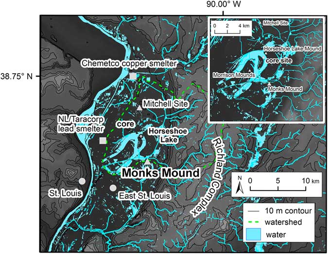
Located near modern-day East St. Louis, Illinois, Cahokia is considered the largest city in the pre-Columbian United States and was the epicenter of the greater Mississippian cultural tradition (Fig. 1). Settlements associated with the Mississippian Tradition are found across the southeastern and midwestern United States, stretching from the Gulf of Mexico to central Wisconsin. The emergence and eventual abandonment of Cahokia and other Mississippian-era settlements has generated questions about the multidirectional relationship between pre-Columbian urbanization and environmental change. For instance, it is unclear to what degree ancient Cahokians affected the landscape through deforestation (Lopinot and Woods, Reference Lopinot and Woods1993; Emerson and Hedman, Reference Emerson and Hedman2016) and were in turn influenced by episodic climate events, such as droughts (Benson et al., Reference Benson, Pauketat and Cook2009) or floods (Munoz et al., Reference Munoz, Schroeder, Fike and Williams2014b). To date there are few well-developed geochemical records associated with the period of initial settlement, major growth, and eventual population decline and abandonment at Cahokia or related Mississippian settlements. To expand our understanding of the environmental impact of humans in North America, we present proxy evidence from a sediment record from Horseshoe Lake.
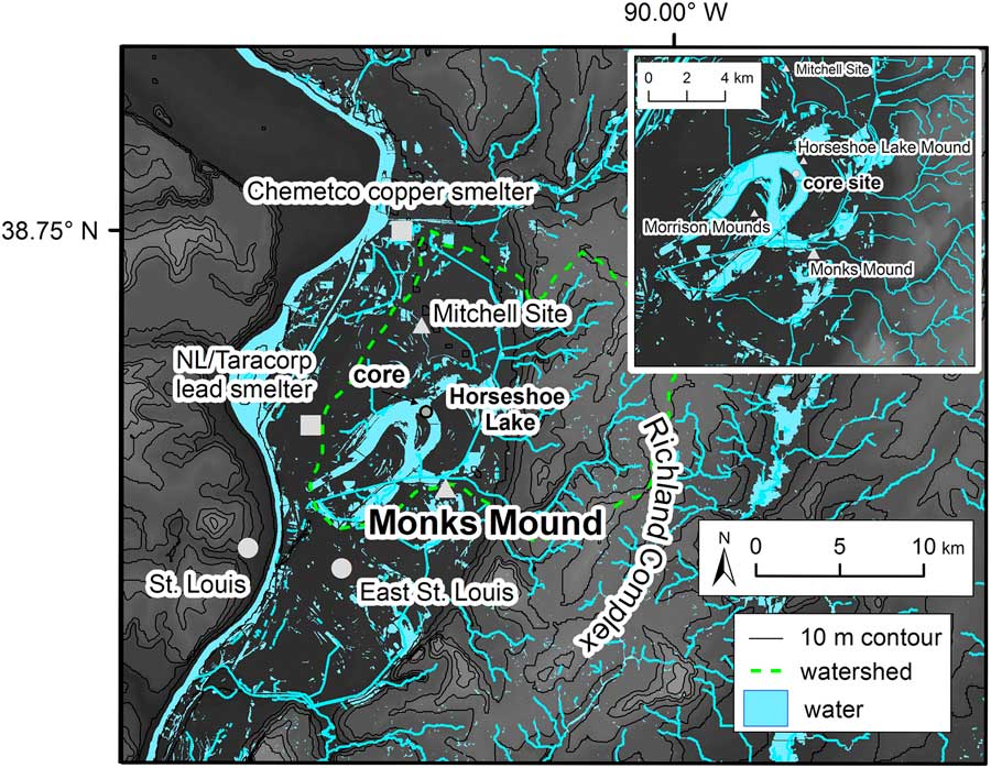
Figure 1. (color online) Map of Horseshoe Lake watershed in relation to Cahokia at Monks Mound and other clusters of earthen mounds in the watershed indicated by triangles. Squares indicate historical smelters. Large circles indicate the location of modern-day cities. The small gray circle in the northeastern part of Horseshoe Lake shows the location of the core site. (Top right) Close-up map of Horseshoe Lake and nearby earthen mounds with core site noted.
The 30-m-high earthwork known as Monks Mound is considered the center of the so-called Greater Cahokia area, which included monumental earthworks, landscaped plazas, and neighborhoods and secondary settlements encompassing more than 1000 hectares (ha) (Milner, Reference Milner1998; Emerson and Hedman, Reference Emerson and Hedman2016; Fig. 1). Occupation of Cahokia can be divided into four distinct phases based on the artifactual record: Lohmann Phase (AD 1050–1100), Stirling Phase (AD 1100–1200), Moorehead Phase (AD 1200–1300), and Sand Prairie Phase (AD 1300–1400) (Fortier et al., Reference Fortier, Emerson and McElrath2006). Major resettlement of Cahokia began during the Lohmann Phase, with the greatest period of population expansion occurring between AD 1050 and 1150, with a maximum population of about 5000 to 15,000 near Monks Mound (Pauketat and Lopinot, Reference Pauketat and Lopinot1997; Milner, Reference Milner1998; Fortier et al., Reference Fortier, Emerson and McElrath2006). The subsequent Stirling Phase is considered to mark Cahokia’s peak (Kelly, Reference Kelly1997), with population estimates of 15,000 to 50,000 for Cahokia and the surrounding American Bottom region (Milner, Reference Milner1998). During this time, palisade walls were constructed around Monks Mound (Iseminger et al., Reference Iseminger, Pauketat, Koldehoff, Kelly and Blake1990) and rebuilt up to four times over the course of 100 years. Around AD 1160 a large portion of Cahokia appears to have been burned during the so-called Great Conflagration (Pauketat et al., Reference Pauketat, Fortier, Alt and Emerson2013). Archaeological evidence suggests a shift to regional decentralization and a decline in the construction of monumental earthworks during the late Stirling Phase (Dalan, Reference Dalan1997; White et al., Reference White, Stevens, Lorenzi, Munoz, Lipo and Schroeder2018). This trend continued through the Moorehead Phase, although Cahokia continued to function as a regional civic–ceremonial center (Pauketat and Lopinot, Reference Pauketat and Lopinot1997). Final abandonment of the city occurred by AD 1400, during the Sand Prairie Phase (Fortier et al., Reference Fortier, Emerson and McElrath2006).
At its height, Cahokia’s urban landscape was marked by a network of earthen mounds, plazas, agricultural fields, and satellite settlements (Pauketat, Reference Pauketat1998). Of particular note is the construction of at least 200 monumental earthworks within a comparatively short period of time, including Monks Mound and an adjacent 20 ha plaza (Fowler, Reference Fowler1997; Dalan et al., Reference Dalan, Holley, Woods, Watters and Koepke2003; Emerson and Hedman, Reference Emerson and Hedman2016). Archaeological evidence suggests that Cahokia peaked and fell into decline by AD 1150 to 1200, yet the reasons behind this decline remain unclear (Benson et al., Reference Benson, Pauketat and Cook2009; Meeks and Anderson, Reference Meeks and Anderson2013; Emerson and Hedman, Reference Emerson and Hedman2016). The area was sparsely populated after approximately AD 1400 until the beginning of European settlement in AD 1696. The last 200 years of European and American settlement further altered the local landscape through a combination of agriculture (e.g., livestock, etc.), industry (e.g., smelting), and flood-control activities (e.g., levees) (Ollendorf, Reference Ollendorf1993).
Setting and background
Horseshoe is an oxbow lake located in the floodplain of the Mississippi River about 13 km east of East St. Louis in the American Bottom. The earthworks and plazas associated with Monks Mound are located just outside the watershed of Horseshoe Lake. Several smaller mound clusters and settlements associated with the growth of Greater Cahokia (Kelly, Reference Kelly1997) are located in the Horseshoe Lake watershed, including the Mitchell site and the Horseshoe Lake Mound site (Ollendorf, Reference Ollendorf1993; Milner, Reference Milner1998; Fig. 1). Though each locality had a unique occupational history, these sites expanded during the coalescence of Greater Cahokia. Therefore, the Horseshoe Lake record reflects changes in the outlying areas surrounding Cahokia and may not fully capture the impact of population centralization and urbanization near the central precinct at Monks Mound.
Today, Horseshoe Lake is shallow (1–5 m) and covers a surface area of about 1200 ha with a watershed area of ~20,000 ha. The eastern side of the watershed drains the Mississippi River terrace bluffs that are composed of loess and sensitive to erosion from agriculture and deforestation (Trimble, Reference Trimble1999; Grimley et al., Reference Grimley, Phillips and Lepley2007). Horseshoe Lake was cut off from the main channel of the Mississippi River about 2400 years ago (Booth and Koldehoff, Reference Booth and Koldehoff1999; Grimley et al., Reference Grimley, Phillips and Lepley2007). Since that time, continual flooding and migration of the main channel has led to a complex geomorphological history for the basin in terms of shoreline shape, lake volume, and flood frequency (Milner, Reference Milner1998). For example, variations in weather patterns and hydrologic conditions in the Mississippi River can cause lake levels to rise and fall. During wet periods and flooding, Horseshoe Lake is surficially open with a high degree of surficial water inflow and outflow. During extended dry periods, the shallow areas of the lake can dry out. Historically, the lake received water from Cahokia Creek, Grassy Lake, Judy’s Branch, Canteen Creek, Little Caseyville Creek, and other drainages on the bluff to the east (Ollendorf, Reference Ollendorf1993). Today, Horseshoe Lake mainly receives runoff through Nameoki Ditch and Elm Slough and treated effluent from the Granite City Steel facilities. During flooding, storm water in the Cahokia Canal is diverted into the lake for flood retention (Hill et al., Reference Hill, Evans and Bell1981). The outflow south of the causeway is maintained by the Metro East Sanitation District (Ollendorf, Reference Ollendorf1993). There is an elevated risk for groundwater contamination at Horseshoe Lake because of the high permeability of the sand and gravel aquifers that underlie the floodplain (Grimley et al., Reference Grimley, Phillips and Lepley2007). The lake water is alkaline with a high pH (~8) (Hill et al., Reference Hill, Evans and Bell1981; Illinois EPA, 2009) resulting in the formation of authigenic carbonate minerals in the water column.
Previous studies have analyzed sediment from Horseshoe Lake (Ollendorf, Reference Ollendorf1993; Vermillion et al., Reference Vermillion, Brugam, Retzlaff and Bala2005; Munoz et al., Reference Munoz, Schroeder, Fike and Williams2014b). Work by Ollendorf (Reference Ollendorf1993) recovered a series of transect cores from the northeastern basin of Horseshoe Lake. The longest cores displayed complex stratigraphy with organic-rich calcareous silt and clay units interbedded with sand layers. These changes were noted on a depth scale, because radiocarbon dating was measured on bulk sediment and shell macrofossils, which were contaminated by the hard-water effect (Deevey et al., Reference Deevey, Gross, Hutchinson and Kraybill1954). Palynological analysis revealed that maize (Zea mays) pollen could be identified and isolated in sediment at depths of up to 4 m, suggesting that the pollen could be prehistoric. However, due to the use of bulk sediment ages, no age estimates were given for the maize pollen found at depth (Ollendorf, Reference Ollendorf1993). Vermillion et al. (Reference Vermillion, Brugam, Retzlaff and Bala2005) and Brugam et al. (Reference Brugam, Bala, Martin, Vermillion and Retzlaff2003) analyzed the last two centuries of sediment using a 210Pb chronology and showed that recent sediments had higher concentrations of heavy metals and a distinct isotopic lead signature compared with lead deposited during the early nineteenth century, indicating contamination of the lake by nearby lead smelting (Fig. 1) and burning of leaded gasoline. White et al. (Reference White, Stevens, Lorenzi, Munoz, Lipo and Schroeder2018) analyzed fecal stanols in the sediment over the last ~1200 years as a proxy for population change around Horseshoe Lake. Fecal stanol population reconstructions appear to be broadly consistent with population reconstructions using archaeological evidence (Pauketat and Lopinot, Reference Pauketat and Lopinot1997; Milner, Reference Milner1998), and suggest a decline in population at Cahokia from AD 1100 to 1400. Munoz et al. (Reference Munoz, Schroeder, Fike and Williams2014b) noted a distinct fine-grained layer in the sediment radiocarbon dated to approximately AD 1200. They attributed the formation of this layer to a large flood on the basis of principal component analysis of grain-size distribution and contemporaneous deposition of a similar layer in nearby Grassy Lake (Munoz et al., Reference Munoz, Gruley, Massie, Fike, Schroeder and Williams2015b). This interpretation of a large flood affecting Cahokia, however, has been called into question (Baires et al., Reference Baires, Baltus and Buchanan2015; Munoz et al., Reference Munoz, Gruley, Fike, Schroeder and Williams2015a; Emerson and Hedman, Reference Emerson and Hedman2016). Using additional sediment evidence with a robust radiocarbon chronology extending 1500 years, we test the large flood hypothesis (Munoz et al., Reference Munoz, Schroeder, Fike and Williams2014b) and show that several proxies support an alternative hypothesis of anthropogenic factors affecting the geochemistry of Horseshoe Lake during Cahokia.
METHODS
Fieldwork
Eight overlapping drives were collected in AD 2012 and 2013 from the easternmost basin (38.6983°N, 90.0731°W) of Horseshoe Lake in 1.3 m of water (Fig. 1). Core A-12 was recovered using a 5.5-cm-diameter piston core with a removable polycarbonate tube to a depth of 1.40 m below the sediment–water interface. The flocculate upper 27 cm of sediment from Core A-12 was extruded in the field at 0.5 cm intervals into Whirl-Pak bags. A steel-barrel Livingstone corer was used to collect overlapping cores from three adjacent core sites (Cores B-12, D-13, and E-13) that consist of a total of seven ~1-m-long drives. Core E-13 consists of two overlapping drives that span the interval from 1.52 to 3.41 m below the sediment–water interface. A composite core was developed by splicing together the A-12 surface core and the E-13 Livingstone cores using visible stratigraphic markers and a magnetic susceptibility profile (Supplementary Fig. S1).
Laboratory work
Sediment cores were transported to the University of Pittsburgh in acrylonitrile butadiene styrene tubing sealed with duct tape. In the laboratory, the cores were removed from the tubing and split lengthwise. The split half surface of the core was scanned for magnetic susceptibility. The cores were then subsampled for proxy analyses. Nine 1-cm-thick samples were taken at mean depths of 26, 42, 196, 203, 207, 210, 211, 212, and 311 cm for X-ray diffraction (XRD).
Magnetic susceptibility was measured on the split-core surface of all the drives at a 0.2 cm interval at room temperature using a Tamiscan high-resolution surface-scanning sensor connected to a Bartington MS2 susceptibility meter at the Department of Geology and Environmental Science, University of Pittsburgh.
Sediment subsamples were collected at 2 to 5 cm intervals down Cores A-12 and E-13 using a 1 cm3 piston sampler and dried for 48 hours at 60°C to calculate dry bulk density. Weight percent organic matter and carbonate content of the dried samples were determined by loss-on-ignition (LOI) analysis at 550°C for 4 hours and at 1000°C for 2 hours, respectively (Heiri et al., Reference Heiri, Lotter and Lemcke2001).
A total of 26 sediment subsamples were analyzed only for maize pollen at the Instituto de Geología, Universidad Nacional Autónoma de México. Only maize pollen was targeted for analysis because of its importance as an indicator of agricultural activity. A volume of 0.5 cm3 was processed following standard protocols for pollen analysis (Faegri and Iversen, Reference Faegri and Iversen1989) and subsequently sieved through a 50 μm mesh. Samples were scanned at 400× and 1000× magnifications using a transmitted light microscope until maize pollen was found or until the entire sample was examined. In addition, a known volume of sediment was extracted for charcoal analysis from the same subsamples analyzed for maize pollen. The sediment was disaggregated using sodium pyrophosphate to separate charcoal particles from the sediments. Charcoal particles were manually separated under a stereo microscope at 50× magnification (Clark, Reference Clark1988). A digital picture of the samples was taken to determine the number of pixels and therefore the area covered by charcoal using ImageJ software (Rasband, Reference Rasband2005). The charcoal area (mm2) was then normalized to volume and expressed in terms of concentration (i.e., mm2/cm3).
Lead (Pb), copper (Cu), potassium (K), and aluminum (Al) concentrations were measured down core at 2 to 5 cm intervals. One interval of interest from 197 to 221 cm was resampled at continuous 1 cm intervals. Metals were extracted from lyophilized and homogenized sediments overnight using ultrapure 10% HNO3. Previous heavy metal analysis of Horseshoe Lake sediment used X-ray fluorescence (XRF) techniques (Brugam et al., Reference Brugam, Bala, Martin, Vermillion and Retzlaff2003; Vermillion et al., Reference Vermillion, Brugam, Retzlaff and Bala2005). The weak nitric acid extraction method differs from XRF analysis in that it targets metals bound to exchange sites (i.e., sorbed) on sediment surfaces (and in the case of Horseshoe Lake also contained in carbonate minerals), which have been shown to be sensitive to anthropogenic inputs (Hilton et al., Reference Hilton, Davison and Ochsenbein1985; Graney et al., Reference Graney, Halliday, Keeler, Nriagu, Robbins and Norton1995). After 24 hours, the sediment–acid mix was centrifuged and the resulting supernatant was subsampled, diluted in 2% HNO3, spiked with an internal standard, and measured for metal concentration. Metals were measured on a PerkinElmer NeXION 300× inductively coupled plasma-mass spectrometer at the Department of Geology and Environmental Science, University of Pittsburgh. Standards, blanks, and duplicates were measured during the analyses to ensure accuracy and reproducibility. Analytical precision is <1 μg/g for Pb, Cu, K, and Al. Only sorbed metal concentrations are presented here.
Weight percent (wt%) nitrogen (N), carbon (C), carbon isotopes (δ13Corg), and nitrogen isotopes of organic matter (δ15Norg) were measured on core subsamples taken at 3 to 5 cm intervals. Subsamples were treated twice with 1 M HCl for 24 hours to dissolve carbonate minerals and rinsed back to neutral pH with deionized water. Samples were then lyophilized and analyzed at the Environmental Isotope Laboratory at the University of Arizona using a continuous-flow gas-ratio mass spectrometer (Finnigan Delta PlusXL) coupled to an elemental analyzer (Costech). Isotope ratios of δ13Corg are reported as ‰ values relative to Vienna Pee Dee Belemnite (VPDB). Nitrogen isotopes of organic matter are expressed in conventional delta (δ) notation as per mil (‰) isotopes and are reported relative to atmospheric N2. Standardization is based on acetanilide for elemental concentration and IAEA-N-1 and IAEA-N-2 for δ15N. Precision is ±0.2‰ for δ15Norg and ±0.12‰ for δ13Corg based on repeated measurements. Precision for wt% C and N is ±0.5%.
Fine-grain carbonate minerals were isolated from the sediments for carbon isotope analysis. This fraction of the sediment is presumed to be composed primarily of authigenic calcite, because there is no nearby limestone bedrock exposed in the watershed that could provide a source of detrital carbonate minerals. Authigenic calcite forms in isotopic equilibrium with the dissolved inorganic carbon (DIC) in the lake water at the time of formation (i.e., δ13CDIC) (Hammarlund et al., Reference Hammarlund, Aravena, Barnekow, Buchardt and Possnert1997). Sediment samples were disaggregated in 7% H2O2 for ~24 hours, wet sieved through a 63 μm screen to remove the biogenic and coarse fraction (and thereby isolate the fine-grain size), decanted, and treated with 3% NaClO for 6 hours to remove organic matter. The sample was then rinsed to neutral pH using deionized water, frozen, lyophilized, homogenized using a razor blade and wax paper, and sealed in labeled glass vials. Samples for carbon isotope measurements of carbonate sediment (δ13CDIC) were reacted in orthophosphoric acid using a Gas Bench II carbonate preparation device. The carbon isotopic composition of evolved CO2 gas was measured with a MAT 252 mass spectrometer at Indianapolis University–Purdue University in Indianapolis. All carbonate isotope results are reported in standard delta notation relative to VPDB. Analytical precision, based on repeated measurements of NBS-18, NBS-19, and IAEA-09 carbonate standard materials was 0.06‰ for δ13C.
The mineralogy of the core was investigated by powder XRD using a Philips X’Pert X-ray diffractometer at the University of Pittsburgh Swanson School of Engineering and at the Large Lakes Observatory at the University of Minnesota Duluth. Nine 1-cm-thick samples were taken at mean depths of 14.75, 26, 196, 203, 207, 210, 211, 212.5, and 314.5 cm and pretreated using 7% H2O2 for 24 h at room temperature to remove organic matter. The sediments were then washed with deionized water, frozen, lyophilized, and homogenized before XRD analysis. The spectra (Supplementary Fig. S2) were analyzed using X’Pert Graphics & Identify and Philips High Score Plus with a phase database from the International Centre for Diffraction Data to identify minerals.
Geochronology
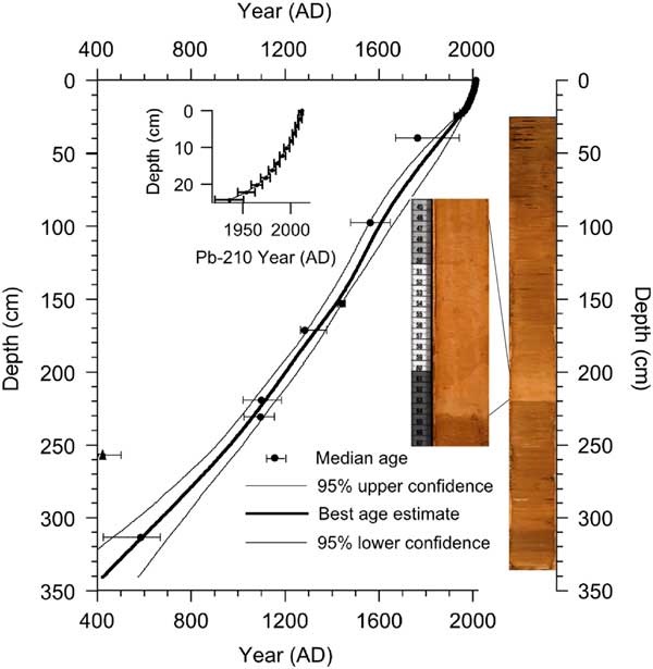
Eight >125 μm charcoal samples were measured for 14C at the Keck Carbon Cycle Accelerator Mass Spectrometry Laboratory at the University of California, Irvine. Before analysis, charcoal samples were pretreated using a standard 1 M HCl, 1 M NaOH, 1 M HCl procedure and rinsed in deionized water to a neutral pH (Abbott and Stafford, Reference Abbott and Stafford1996). A total of 14 samples from the upper 25 cm of extruded sediment from the top of Core A-12 were lyophilized, sealed in airtight dishes for 3 weeks, and measured for 210Pb and 214Pb activities by direct gamma counting for 24 hours in a broad-energy germanium detector (Canberra BE-3825) at the Department of Geology and Environmental Science, University of Pittsburgh. The unsupported 210Pb (i.e., 210Pb minus 214Pb) assays were interpreted using the constant rate of supply (CRS) model (Binford, Reference Binford1990). The resulting ages (Tables 1 and 2) were input into Classical Age Modeling code (CLAM v. 2.2) for R to generate an age model (Blaauw, Reference Blaauw2010; Fig. 2). A smooth spline (tension=0.8) was used to interpolate between the age constraints (Tables 1 and 2) and generate 95% confidence intervals.
Table 1 Horseshoe Lake constant rate of supply (CRS) 210Pb ages.

Table 2 Horseshoe Lake radiocarbon ages.
a This is the median of the 95% calibration (CALIB 7.1) distribution (Stuiver et al., Reference Stuiver, Reimer and Reimer2015).
b Age omitted from the age model.

Figure 2. (color online) The Horseshoe Lake 14C and 210Pb age model compared with a composite core image. Seven radiocarbon ages were input into CLAM v. 2.2 for R and interpolated using a spline (tension=0.8) (Blaauw, Reference Blaauw2010). The triangle indicates the age omitted from the age model. The gray disturbance layer is found at a depth of 197 to 221 cm. Two charcoal radiocarbon ages were recovered below and above the disturbance layer to estimate the age (i.e., nos. 141370, 116877, 141371, 141372).
RESULTS
Age model
The age to depth model was generated in CLAM (v. 2.2) using 8 radiocarbon ages and 14 CRS 210Pb ages (Blaauw, Reference Blaauw2010; Fig. 2). One radiocarbon age was omitted because of an anomalously old age in the context of the other seven ages. The apparent old age suggests that the macrofossil was contaminated with radiocarbon-dead carbon (Deevey et al., Reference Deevey, Gross, Hutchinson and Kraybill1954) or represents reworked material that does not reflect the true age of deposition. Inclusion of this age would require an abrupt change in sediment accumulation that is not supported by any lithological evidence or other radiocarbon measurements. From AD 450 to 1350 (336 to 168 cm depth), the sedimentation rates were 0.19 cm/year on average. After AD 1350 (168 to 0 cm), average sedimentation rates increased to 0.27 cm/year. The 95% confidence interval associated with critical ages related to the timing of anthropogenic changes recorded in the sediment are shown in the text. These were rounded to the nearest 10th digit, because calibrated radiocarbon ages can provide a nonnormal probability distribution, which would require providing two different error values for the upper and lower limits. We included a table in the Supplementary Material that details confidence intervals associated with each age estimate for every 1-cm-thick sediment layer (Supplementary Table S1).
Sedimentology
The sediment consists of homogeneous fine-grained (clay to silt) calcareous and silicate mineral matter and contains shells from freshwater gastropods, bivalves, and ostracods. A 1-cm-thick layer deposited around AD 1480 contains Typha macrofossil remains. The exception to the otherwise homogeneous stratigraphy occurs with the sudden deposition of a distinct fine-grained (clay to silt) gray-colored 24-cm-thick layer (Fig. 2) that is dated (±95% confidence) from AD 1150 ± 50 (197 cm) to AD 1220 ± 50 (221 cm). The base of the gray layer consists of an inclined linear contact with the underlying sediments. About 2.5 cm above this basal contact there is another irregular and inclined sediment transition demarcated by a change in color that gradually fades into darker-colored sediment (Fig. 2). Comparable stratigraphy was also noted by Ollendorf, who collected cores from a similar location (Ollendorf, Reference Ollendorf1993). Samples for powder XRD analysis were taken from composite depths dated to AD ~610, 1150, 1160, 1160, 1171, 1190, 1220, 1940, and 1982. These analyses indicate that the mineral component of the sediment is composed primarily of quartz, calcite, and kaolinite.
AD 450 to 1050
The oldest analyzed sediment corresponds to the Woodland period before population expansion and mound construction at Cahokia. At this depth, background Pb (10 μg/g), Cu (13 μg/g), K (245 μg/g), and Al (2040 μg/g) concentrations are low and at stable average concentrations (Fig. 3). Sediments are composed of 8% organic matter, 12% CaCO3, and 80% residual mineral matter. Carbon/nitrogen ratios (C/N) are at average values of 13 from approximately AD 450 to AD 650 and decrease to 9 by AD 1050 (Fig. 4). Magnetic susceptibility declines overall from AD 450 to 1050. δ15Norg and δ13Corg values are low and stable during this period, with average values of 1.7‰ and −25.0‰, respectively. Similarly, δ13CDIC values remain relatively constant (average value of −2‰), except for a 2‰ increase from AD 950 to 1000. Maize pollen is found in three of the six samples dated to AD 610, 790, and 1040 (Fig. 3).
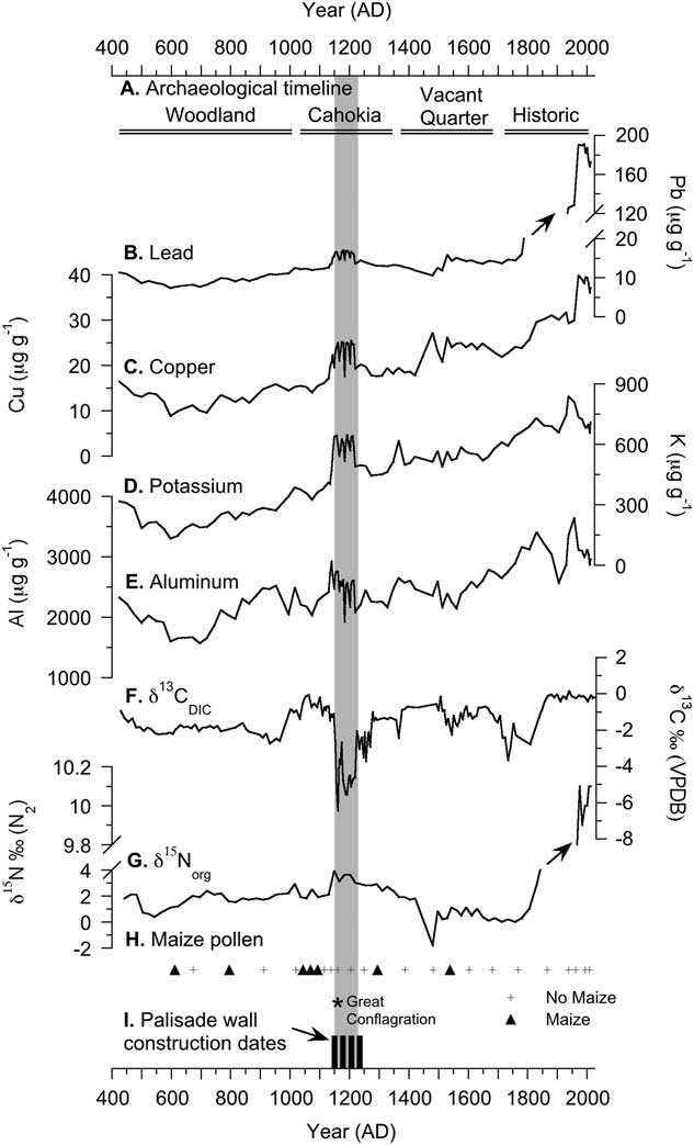
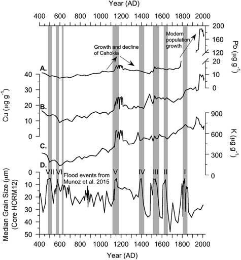
Figure 3. Results from the Horseshoe Lake sediment core for proxies that are sensitive to anthropogenic processes. The gray rectangle indicates the extent of the disturbance layer. Inset horizontal lines (A) indicate archaeological and historical phases in the region. Concentrations of sorbed lead (B), copper (C), potassium (D), aluminum (E), carbon isotopes (F), and nitrogen isotopes (G) are compared with the presence of fossil maize (Zea mays) pollen (H). The timing of the so-called Great Conflagration or large-scale burning of Cahokia (ca. AD 1160) (Pauketat et al., Reference Pauketat, Fortier, Alt and Emerson2013) and the construction of palisade walls (I) (Iseminger, Reference Iseminger2010; Iseminger et al., Reference Iseminger, Pauketat, Koldehoff, Kelly and Blake1990) coincide with the deposition of the disturbance layer. Mud and wood palisade walls were constructed around Monks Mound (Fig. 1) at least four times over the course of ~100 years, each construction requiring the use of around 15,000 to 20,000 oak and hickory logs (~0.3 m in diameter and ~6.0 m long) from the surrounding area.

Figure 4. Horseshoe Lake control proxies including (A) carbon isotopes (δ13Corg), (B) charcoal particulates, (C) C/N, (D) loss-on-ignition, (E) and magnetic susceptibility. The gray rectangle indicates the extent of the gray disturbance layer related to Cahokia. The control proxies do not record distinctive changes during this time.
AD 1050 to 1350
From approximately AD 1050 to AD 1150, sorbed concentrations of Pb, Cu, K, and Al remain similar to average values from AD 450 to 1050. Starting at AD 1150, Pb (14 μg/g), Cu (25 μg/g), K (600 μg/g), and Al (3000 μg/g) rise in concentration and remain elevated until AD 1220 (Fig. 3). Afterward, Cu, K, and Al concentrations decrease. Similarly, starting around AD 1150, δ15Norg shifts to higher values (3.9‰) and remains elevated until approximately AD 1300. δ13CDIC and magnetic susceptibility, however, decrease 5‰ and 8 SI×10−5 from AD 1150 to 1220. δ13Corg is relatively higher on average (−23.8‰). C/N ratios, organic matter, CaCO3, and mineral matter change little from AD 1150 to 1350 (Fig. 4). Maize pollen is detected in three of the eight samples dated to AD 1070, 1090, and 1290 (Fig. 3).
AD 1350 to 1808
Sorbed Pb remains at stable and low concentrations, while Cu and K concentrations gradually increase. Carbon isotope values are elevated on average (−1‰). A 1-cm-thick layer rich in Typha macrofossils (Fig. 3) corresponds with a 2‰ decrease in δ15Norg and slightly higher C/N values (~10). Other than this layer, δ15Norg, C/N, and magnetic susceptibility values remain stable. LOI records increasing organic matter concentrations (~28%) with corresponding shifts to lower mineral matter and CaCO3 concentrations (Fig. 4). Sorbed Al concentrations remain stable and begin to increase around AD 1750. δ13CDIC values decrease by 2‰ around AD 1725 and then begin to increase by AD 1800. Similarly, δ13Corg values decrease gradually over this period to a low of −25.7‰ before increasing ca. AD 1800. Maize pollen is detected in only one of six samples and is dated to AD 1540 (Fig. 3).
AD 1808 to 2012
The outstanding features of this interval include a spike in C/N to 12.5 at AD 1880 (Fig. 4) and an increase in both sorbed Pb and δ15Norg to values about 10 times greater than the average concentrations deposited during the previous ~1500 years (i.e., 145 μg/g and ~10 ‰, respectively) (Fig. 3). Magnetic susceptibility values increase from AD 1850 to 1930 to 66 SI×10−5 (the top of the core was not analyzed, because sediments were extruded in the field). Copper concentrations increase to 10 μg/g from AD 1950 to 1970, while K concentrations remain stable. Aluminum concentrations and δ13CDIC are variable, but elevated after AD 1900. From AD 1860 to 2009, CaCO3 concentrations increase to 24% (Fig. 4), while δ13Corg values are higher (−22.9‰) by AD 1860 and decrease to −26.4‰ by AD 2013. Interestingly, none of the five samples analyzed contain maize pollen (Fig. 3), despite historical records and field observations indicating that maize existed around the lake during the modern period.
DISCUSSION
Core stratigraphy
In the eastern basin of Horseshoe Lake (Fig. 1), the age model and sedimentology indicate that sediment was deposited continuously over the last 1500 years (Fig. 2, Tables 1 and 2), despite historical indications that some parts of the lake may have dried out for extended periods. The sediments in Horseshoe Lake are fine-grained and dark gray-brown (Munsell color 7.5 yr 4/0), with the exception of a distinct gray (7.5 yr 6/0) layer deposited from approximately AD 1150±50 to AD 1220±50 (Fig. 2) that is enriched in δ15Norg, sorbed Pb, Cu, K, and Al, and anomalously low in δ13CDIC. The deposition is contemporaneous with a period of relatively high population density at Cahokia and the surrounding American Bottom region during the Stirling Phase (AD 1100–1200) (Fortier et al., Reference Fortier, Emerson and McElrath2006), which coincides with the construction of hundreds of monumental earthworks (Pauketat, Reference Pauketat1998; Emerson and Hedman, Reference Emerson and Hedman2016) and the abandonment of the Richland Complex on the uplands east of the lake (Pauketat, Reference Pauketat2003). We suggest that geochemical changes documented in the sediment at Horseshoe Lake are consistent with an anthropogenic signal of land use disturbance. For example, the Maya Clay deposits are found in lakes with watersheds that were heavily impacted by human activities and are thought to reflect soil weathering that resulted from widespread human-mediated deforestation (Brenner et al., Reference Brenner, Rosenmeier, Hodell and Curtis2002). The terrace bluffs in the eastern part of the Horseshoe Lake watershed are composed of loess (Bettis, Reference Bettis2003; Fig. 1) and are subject to severe erosion (Krumm, Reference Krumm1984). Erosion can lead to transportation of sediment from steep upland streams to the floodplain, causing siltation in the bottomland wetlands (Lopinot and Woods, Reference Lopinot and Woods1993; Delcourt and Delcourt, Reference Delcourt and Delcourt2004; Peacock et al., Reference Peacock, Haag and Warren2005; Grimley et al., Reference Grimley, Phillips and Lepley2007; Emerson and Hedman, Reference Emerson and Hedman2016). Modern observations indicate that sediment fluxes to streams in the Mississippi River watershed are sensitive to deforestation and agriculture (Knox, Reference Knox1977; Trimble, Reference Trimble1999; Grimley et al., Reference Grimley, Phillips and Lepley2007). On the basis of the sedimentology and proxy indicators that follow, we interpret the sediment record from Horseshoe Lake in the context of supporting documentation from regional historical and archaeological records.
Sorbed metal concentrations
To assess the provenance of the sorbed metal increases, we compared down-core measurements with historical events that have been shown to impact metal deposition in Horseshoe Lake (Brugam et al., Reference Brugam, Bala, Martin, Vermillion and Retzlaff2003; Vermillion et al., Reference Vermillion, Brugam, Retzlaff and Bala2005). Sorbed Pb concentrations increase in Horseshoe Lake sediments after approximately AD 1800 (Fig. 3) and are strongly associated with human population growth (Supplementary Table S2) in the townships adjacent to the lake. Historical inputs of lead to the lake were likely sourced from smelting in combination with burning leaded gasoline (March, Reference March1967; Farquhar et al., Reference Farquhar, Walthall and Hancock1995; Vermillion et al., Reference Vermillion, Brugam, Retzlaff and Bala2005). The increase in sorbed Cu concentration around AD 1970 corresponds with the opening of the Chemetco copper smelter near Harford, Illinois, in AD 1969 (US EPA, 2014; Fig. 1). Following the closure of the nearby lead smelter in AD 1983 (US EPA, 1990), the removal of lead in gasoline (Kovarik, Reference Kovarik2005), and the closure of the copper smelter in AD 2001 (US EPA, 2014), concentrations of both Pb and Cu decline, but remain at relatively high concentrations compared with the previous ~1500 years (Fig. 3). The close correspondence between the metals and the historical record suggest that the sediments at Horseshoe Lake record both the timing and magnitude of anthropogenic metal inputs.
From AD 500 to 1800, sorbed metal concentrations remain relatively low, with the exception of approximately AD 1150 to AD 1220 when Pb, Cu, K, and Al record a distinctive and concomitant increase (Fig. 3). The rise in sorbed metal concentrations coincides with the expansion of Greater Cahokia (along with associated settlements and agriculture) and construction of large earthen mounds (Milner, Reference Milner1998; Emerson and Hedman, Reference Emerson and Hedman2016; Fig. 1). The combination of these activities likely exposed vast quantities of soils in the watershed of Horseshoe Lake, which shifted the source of sorbed metals delivered to the lake. Archaeological excavations on the upland river terraces in the eastern part of the Horseshoe Lake watershed (referred to as the Richland Complex) indicate that this area was abruptly settled and potentially deforested for farming during the Lohmann and Stirling Phases (AD 1050–1150) (Pauketat, Reference Pauketat2003). Therefore, the increase in sorbed metals following the abandonment of the Richland Complex is consistent with human-driven landscape change.
The concentration of sorbed metals in lake sediments can be affected by changing organic matter content and grain-size variations, because these factors strongly control the cation-exchange capacity of the sediment (Bloom, Reference Bloom1981; Helios Rybicka et al., Reference Helios Rybicka, Calmano and Breeger1995; Wang et al., Reference Wang, Jin, Bu, Zhou and Wu2006), and therefore could potentially obscure metal signals liberated from sediment in a 10% HNO3 extraction. To account for these factors, we analyzed organic matter (Fig. 4) and compared sorbed metals with grain-size measurements from the previously published HORM12 core (Munoz et al., Reference Munoz, Schroeder, Fike and Williams2014b, Reference Munoz, Gruley, Massie, Fike, Schroeder and Williams2015b; Fig. 5). Trends in both percent organic matter and changes in grain size do not correspond with changing sorbed metal concentrations through time. Instead, the trends in sorbed metal concentrations appear to be consistent with changing human populations in the watershed documented historically and in the archaeological record. This observation is supported by other studies (Martinez-Cortizas et al., Reference Martinez-Cortizas, Garcia-Rodeja, Pombal, Munoz, Weiss and Cheburkin2002; Pompeani et al., Reference Pompeani, Abbott, Steinman and Bain2013; Hillman et al., Reference Hillman, Yu, Abbott, Cooke, Bain and Steinman2014; Cooke and Bindler, Reference Cooke and Bindler2015), which found that anthropogenic metal signals extracted from sediment in weak acid are largely invariant to changes in organic matter and mineral content.
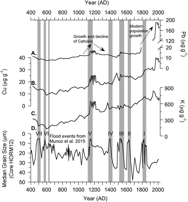
Figure 5. Sorbed lead (A), copper (B), and potassium (C) concentrations compared with the median grain-size record from the nearby HORM12 core (D) (Munoz et al., Reference Munoz, Schroeder, Fike and Williams2014b, Reference Munoz, Gruley, Massie, Fike, Schroeder and Williams2015b). Shifts to fine grain size (highlighted in gray) are interpreted to reflect flooding events (Munoz et al., Reference Munoz, Gruley, Massie, Fike, Schroeder and Williams2015b). Shifts in grain size do not explain trends in sorbed metal concentrations. Rather, increase in sorbed metal concentrations appear to reflect changing human activity.
The period of higher sorbed Cu concentration in the sediment from AD 1150 to 1220 is contemporaneous with evidence for a copper workshop near Monks Mound (Kelly and Brown, Reference Kelly and Brown2010; Fig. 1). We raise the possibility that copper deposited in the sediment during this time may, in part, be derived from metalworking (e.g., annealing [Peterson, Reference Peterson2003; Chastain et al., Reference Chastain, Deymier-Black, Kelly, Brown and Dunand2011]) and biomass burning for several reasons. The concomitant increase in sorbed Pb and K concentrations are consistent with a prehistoric metalworking signal recorded in lake sediments near prehistoric copper mines in North America (Pompeani et al., Reference Pompeani, Abbott, Bain, DePasqual and Finkenbinder2015). In addition, K concentrations have been used to infer biomass burning in ice cores (Eichler et al., Reference Eichler, Brütsch, Olivier, Papina and Schwikowski2009; Kehrwald et al., Reference Kehrwald, Zangrando, Gabrielli, Jaffrezo, Boutron, Barbante and Gambaro2012), because fine aerosol K (<1 μm) is found in relatively high concentrations in smoke (Larson and Koenig, Reference Larson and Koenig1994; Kleeman et al., Reference Kleeman, Schauer and Cass1999). Furthermore the rise in Cu, Pb, and K occur in the absence of large changes in C/N ratio, organic matter concentrations, and magnetic susceptibility (Figs. 4 and 5), indicating that increases in sorbed metal concentrations are not influenced by large changes in organic matter or mineral composition of the sediment. There is little archaeological evidence, however, for an intensive copper industry beyond a single copper workshop excavated near Monks Mound (Kelly and Brown, Reference Kelly and Brown2010). Additionally, copper artifacts are rare in the archaeological record. Therefore, the relatively small increase in sorbed metals in the sediment from AD 1150 to 1220 is consistent with a small-scale industry and suggests that Cahokia had a lesser impact on the metal cycle compared to modern activities. At this time it is difficult to distinguish the proportion or amounts of metals derived from dissolved transport in ground and surface water (via weathering and erosion) versus airborne fallout. Nevertheless, both transport mechanisms are consistent with historically documented industrial activities (e.g., smelting) and archaeological evidence (e.g., mound building, biomass burning, metalworking), both of which resulted in measureable changes in sorbed metal delivery to the lake.
Nitrogen isotopes
After AD 1810, δ15Norg values in Horseshoe Lake sediment increase until the present in association with human population growth around the lake (Anonymous, Reference Anonymous1882; Supplementary Table S2). Shifts to higher δ15Norg values over the last ~200 years reflect groundwater contamination with sewage nitrate from outhouses and septic systems via sand and gravel aquifers (i.e., the Henry and Cahokia Formations) that underlie Horseshoe Lake and the surrounding floodplain (Brugam et al., Reference Brugam, Bala, Martin, Vermillion and Retzlaff2003; Elliott and Brush, Reference Elliott and Brush2006; Grimley et al., Reference Grimley, Phillips and Lepley2007; Widory et al., Reference Widory, Petelet-Giraud, Negrel and LaDouche2005). Groundwater contamination with human waste is supported by LOI and C/N, which do not increase along with δ15Norg, indicating that the delivery of terrestrial organic matter or changes in primary productivity did not cause higher δ15Norg values (Figs. 4 and 5). Rather, the data suggest that higher δ15Norg values are due to changes in the isotopic composition of dissolved nitrogen delivered in groundwater to Horseshoe Lake. Additional factors that could affect δ15Norg values include transport processes such as precipitation, temperature (Craine et al., Reference Craine, Elmore, Aidar, Bustamante, Dawson, Hobbie and Kahmen2009), agricultural land cover, fertilizer application rate (Dumont et al., Reference Dumont, Harrison, Kroeze, Bakker and Seitzinger2005), soil type, biological communities, irrigation activities (Evans, Reference Evans2007), and airborne nitrogen deposition from burning biomass and fossil fuels (during the twentieth century) (Elliott et al., Reference Elliott, Kendall, Boyer, Burns, Lear, Golden, Harlin, Bytnerowicz, Butler and Glatz2009; Felix and Elliott, Reference Felix and Elliott2013). Furthermore, nitrogen undergoes isotopic fractionation by organisms during and after sedimentation (Elliott and Brush, Reference Elliott and Brush2006). The strong relationship between δ15Norg values and human population growth following Euro-American settlement suggests some type of anthropogenic nitrogen as the primary factor contributing to the observed increase in δ15Norg (Brugam et al., Reference Brugam, Bala, Martin, Vermillion and Retzlaff2003).
δ15Norg values increase ca. AD 1150 during the late Stirling Phase (AD 1100–1200), which is considered a period of relatively high population density at Cahokia and in the larger American Bottom region (Milner, Reference Milner1998). δ15Norg values remain elevated for two centuries before returning to predisturbance levels by approximately AD 1350. Based on this correspondence between the geochemical and archaeological records, we suggest a connection between δ15Norg and fluctuations in human population within the Horseshoe Lake watershed. Sewage and other wastes were deposited in borrow pits (Pauketat, Reference Pauketat1998, Reference Pauketat2003), where the reactive nitrogen and other compounds, such as coprostanol (White et al., Reference White, Stevens, Lorenzi, Munoz, Lipo and Schroeder2018), could contaminate groundwater and eventually be delivered to the lake sediments. Furthermore, Leguminosae (bean) cultivation starting around AD 1300 may have enhanced inputs of reactive nitrogen to soils, but contributions from this source are poorly constrained and are assumed to be negligible. Shifts to higher sediment δ15Norg at Horseshoe Lake from AD 1150 to 1350 therefore are interpreted to be related to higher population densities in the watershed.
Carbon isotopes of DIC
The δ13C of DIC in lake water is preserved in authigenic carbonate minerals that form in the water column at Horseshoe Lake. The minerals accumulate in the sediment and archive the changing isotopic composition of lake DIC over time. Lake water DIC is affected by sources and processes such as bedrock geology, vegetational composition, productivity, soil, and groundwater throughflow (e.g., Hammarlund et al. Reference Hammarlund, Aravena, Barnekow, Buchardt and Possnert1997). For example, the conversion of forests to cultivated land can liberate soil carbon (Murty et al., Reference Murty, Kirschbaum, McMurtrie and McGilvray2002), which can percolate into groundwater delivered to lakes. Contributions of carbon dioxide from soil respiration in groundwater are generally more isotopically negative than sources found in lake water (Salomons and Mook, Reference Salomons and Mook1991). In closed-basin lakes, changes in hydrologic balance such as increased evaporation can also cause increases in the δ13C values of DIC (Li and Ku, Reference Li and Ku1997) and the resultant δ13C of authigenic carbonates. The influence of burning biomass on the δ13C of DIC is presumed to be negligible, because combustion releases mainly inert carbon compounds (with respect to DIC) and gaseous carbon (e.g., carbon monoxide) (Larson and Koenig, Reference Larson and Koenig1994) that are transported out of the watershed. Carbon sourced from sewage is likely similar to the composition of source foods, because fractionation of carbon isotopes during digestion is negligible (≤1‰) (Sponheimer et al., Reference Sponheimer, Robinson, Ayliffe, Passey, Roeder, Shipley, Lopez, Cerling, Dearing and Ehleringer2003).
The 5‰ decline and sustained low δ13CDIC values in Horseshoe around AD 1150 are the most negative values found in the entire sediment record. We interpret the large depletion in δ13CDIC to be the result of mound building and agriculture, which likely increased the respiration of soil organic matter, thereby adding isotopically light carbon to groundwater and lake DIC (Dubois et al., Reference Dubois, Lee and Veizer2010; Fig. 3). It is unlikely that the large shift to more negative δ13CDIC values at approximately AD 1150 solely reflects changes in lake hydrology, given that there is no geomorphological or sedimentological evidence for a major rise or fall in lake level at this time. Nor could it reflect changes in algal productivity, given that δ13Corg and LOI are largely invariant. Interestingly, the decline in δ13CDIC is not associated with large changes in C/N (Figs. 4 and 5), indicating the disturbance primarily affected the inorganic carbon cycle at Horseshoe Lake. Isotopic and archaeobotanical evidence suggests the importance of maize (a C4 plant) consumption during the Mississippian Period (Yerkes, Reference Yerkes2005; Emerson and Hedman, Reference Emerson and Hedman2016). Despite archaeological and osteological evidence for maize consumption, sediment δ13CDIC at Horseshoe does not shift toward enriched δ13C values that are characteristic of C4 plants. This suggests that another factor, such as the enhanced respiration of isotopically light soil organic matter, is most likely responsible for the observed changes to lake DIC.
Carbon isotopes of organic matter
Carbon isotopes of organic matter (δ13Corg) are low on average (−25.2‰) from AD 440 to approximately AD 1000, before shifting to higher average values (−24.4‰) until the present. There is a nearly 3‰ shift between data points ca. AD 1000. No notable changes in δ13Corg are detected from AD 1150 to 1220 (Fig. 4), when other proxies (i.e., sorbed metal concentrations, δ15Norg, δ13CDIC) suggest human-induced changes in the catchment. There is a +3‰ shift, however, in δ13Corg from AD 1800 to 1850, which may reflect early Euro-American land use. After AD 1850, despite continued population growth around the lake (Supplementary Table S2), δ13Corg declined back to values that were recorded before Euro-American settlement in the region. We conclude that the δ13Corg may not be sensitive to the landscape disturbance indicated by sorbed metal concentrations, δ15Norg, and δ13CDIC.
Maize pollen and charcoal analysis
We analyzed maize pollen presence as an indicator of agricultural activity. The poor correspondence of maize pollen with the historical record demonstrates that its absence in the sediment sample analysis does not necessarily indicate absence of cultivation near the lake. This is partially due to the large size and limited aerial distribution of maize pollen (Lane et al., Reference Lane, Cummings and Clark2010). Maize pollen, however, was identified in 7 of the 25 sediment samples analyzed from Horseshoe Lake, with the earliest samples dated to AD 610 and 790 (Fig. 3). The ages presented here for maize pollen occur several centuries before verifiable maize remains radiocarbon dated to approximately AD 980 at the Holding Site located ~4 km east of Horseshoe Lake (Riley et al., Reference Riley, Gregory, Bareis, Fortier and Parker1994; Simon, Reference Simon2017). Interestingly, maize pollen was also identified in a layer dated to AD 1540 after the abandonment of Cahokia. Maize pollen is not detected in the disturbance layer dated to AD 1150–1220.
Charcoal was counted from the same sediment intervals that were analyzed for maize pollen. Charcoal concentrations were high and variable from AD 600 to 1200, and low from AD 1200 to 1700, before increasing again after AD 1700. Large increases in visible charcoal concentrations likely reflect wildfires (Whitlock and Anderson, Reference Whitlock and Anderson2003) or potentially large-scale burning events caused by humans. However, there is no distinct increase in charcoal from a sample dated to AD 1150–1220 (Fig. 4), when the other proxies and the archaeological record indicate human impact to the lake. Human-related inferences based on macroscopic charcoal alone are complicated by several factors that may explain why the metals/isotopes appear to record a signal separate from the charcoal. First, our sampling resolution of charcoal is much lower than for the other proxies. Only one sample was obtained from the AD 1150–1220 layer; therefore, our analysis does not record variation in fine-resolution charcoal concentrations that may be more sensitive to human activity. Additionally, transport and preservation of charcoal to lakes is sensitive to sediment flux, weather, and fire/fuel characteristics (Whitlock and Anderson, Reference Whitlock and Anderson2003). For example, hydrologic conditions (e.g., open vs. closed basin) and water depth can affect the flux of charcoal to the sediments in lakes such as Horseshoe Lake by changing the energetic conditions in the water column, thereby preventing preservation of charcoal in the sediment. Typically, charcoal >125 μm in size is used to reconstruct forest fires around lakes, because strong updrafts created by large fires can transport visible charcoal pieces several kilometers (Clark, Reference Clark1988). Large concentrations of charcoal deposited in lake sediment are commonly interpreted to result from a large proximal forest fire (Whitlock and Anderson, Reference Whitlock and Anderson2003). Small controlled fires, such as domestic wood burning for cooking or warmth, likely do not emit as much >125 μm charcoal. The vast majority of wood smoke emissions consists of gases and particulates <1 μm (Larson and Koenig, Reference Larson and Koenig1994; Kleeman et al., Reference Kleeman, Schauer and Cass1999). Thus, charcoal concentrations are not sensitive to controlled, low-intensity fires. Previous research has found that metals derived from atmospheric fallout are most frequently present as particulates, which are most commonly sorbed to clay surfaces and organic matter (Hilton et al., Reference Hilton, Davison and Ochsenbein1985). Our geochemical analysis specifically targets these particulates, which have been shown to reflect human inputs (Graney et al., Reference Graney, Halliday, Keeler, Nriagu, Robbins and Norton1995). We suggest that the geochemical response of Horseshoe Lake is consistent with what we would expect from an anthropogenic signal despite the lack of evidence for increased charcoal concentrations in the sediment layer dated to AD 1150–1220.
Flood hypothesis
Horseshoe Lake contains fine-grained sediment composed of clay to silt (Munoz et al., Reference Munoz, Schroeder, Fike and Williams2014b; Fig. 5). These are grain sizes that would be expected for a backwater oxbow lake (Gilli et al., Reference Gilli, Anselmetti, Glur and Wirth2013). We hypothesize that floods would inundate Horseshoe Lake more frequently soon after being cut off from the Mississippi River, because the lake would be closer to the active channel (Milner, Reference Milner1998). We predict that flood deposits would increase the delivery of terrestrial sediment to the lake, leading to higher magnetic susceptibility values (Gilli et al., Reference Gilli, Anselmetti, Glur and Wirth2013) and C/N ratios (Meyers, Reference Meyers1997; Osleger et al., Reference Osleger, Heyvaert, Stoner and Verosub2009). As the river migrated away, flooding would deliver less terrestrial material to the lake as the distance between the active channel and the basin became greater. This prediction is supported by the sediment proxies, which display higher magnetic susceptibility values and C/N ratios early in the record from AD 450 to 1000 (2.5–3.4 m) (Fig. 4). Higher and more variable magnetic susceptibility values are also recorded in deeper sediment (3.5–5.75 m; core HORM 12) deposited soon after Horseshoe Lake was cut off from the Mississippi River (Munoz et al., Reference Munoz, Schroeder, Fike and Williams2014b). The decline in magnetic susceptibility and C/N ratios after AD 1000 indicates a reduction in flood-sediment input. This suggests that high magnetic susceptibility values and C/N ratios can be used to differentiate zones in the core that contain relatively higher amounts of flood sediment.
Munoz et al. (Reference Munoz, Schroeder, Fike and Williams2014b) observed the fine-grained disturbance layer dated to AD 1200 in a different set of sediment cores from Horseshoe Lake and interpreted it to represent a flood deposit. The basis for their interpretation was fine sediment grain size, low pollen concentration, and the presence of a similar layer in cores recovered from other areas within the Horseshoe Lake basin. The interpretation that this layer formed as a result of a flood event is problematic for several reasons: (1) Horseshoe Lake is located in the floodplain of the Mississippi River and flooded several times before the construction of levees (e.g., AD 1785, 1844) (National Oceanic and Atmospheric Administration [NOAA], 2014), suggesting flood deposits (Fig. 5) should be present throughout the 1500-year-long sediment core. Munoz et al. (Reference Munoz, Schroeder, Fike and Williams2014b) interpret the accumulation of a fine-grained sediment layer from approximately AD 1800 to AD 1850 as a flood deposit, because the timing broadly coincides with a flood that occurred on June 27, 1844; however, sediment grain size fails to distinguish another flood event with a similar stage that occurred on April 1, 1785 (NOAA, 2014). This indicates that the relationship between sediment grain size and flooding is more complex than Munoz et al. (Reference Munoz, Schroeder, Fike and Williams2014b) suggest and may not reliably distinguish individual flood deposits (Gilli et al., Reference Gilli, Anselmetti, Glur and Wirth2013). (2) Four radiocarbon ages of charcoal constrain the ages of the upper and lower contacts of the fine-grained layer deposited ca. AD 1200. These ages do not indicate rapid deposition as suggested by Munoz et al. (Reference Munoz, Schroeder, Fike and Williams2014b), but rather accumulation over an approximately 70 year period (Fig. 2, Table 2). (3) Additional work by Munoz et al. (Reference Munoz, Gruley, Massie, Fike, Schroeder and Williams2015b) identified a similar layer dated to the same period from at least one floodplain lake (i.e., Grassy Lake) located near late prehistoric population centers south of Cahokia. We propose that the contemporaneous deposition of a fine-grain sediment layer at both sites may suggest widespread land-use change associated with regional population growth, rather than a large-scale flood. For example, analysis of sediment profiles in Central America have detected the so-called Maya Clay layers in lakes and wetlands found across a relatively large geographic area (Brenner, Reference Brenner1983; Jacob, Reference Jacob1995; Rosenmeier et al., Reference Rosenmeier, Hodell, Brenner, Curtis and Guilderson2002; Fleury et al., Reference Fleury, Malaizé, Giraudeau, Galop, Bout-Roumazeilles, Martinez, Charlier, Carbonel and Arnauld2014; Beach et al., Reference Beach, Luzzadder-Beach, Cook, Dunning, Kennett, Krause, Terry, Trein and Valdez2015). However, further geochemical analysis of Grassy Lake sediment is needed to rule out this possibility. (4) A flood interpretation is inconsistent with archaeological evidence; there are no peer-reviewed archaeological reports that describe the excavation of a distinct layer attributable to a major flood around AD 1200 (Dalan et al., Reference Dalan, Holley, Woods, Watters and Koepke2003; Baires et al., Reference Baires, Baltus and Buchanan2015). Considering the distinct signal in the sediment, and the fact that Cahokia is one of the most extensively excavated archaeological sites in the United States, it is perplexing that there is no evidence for a large-scale flood that dates to the late Stirling Phase (because it would accumulate in depressions like midden pits). (5) C/N ratios and magnetic susceptibility values remain low (Fig. 4) throughout the layer dated to AD 1150–1220, indicating that it was not formed during a flood.
Taken together, these lines of evidence, along with the other geochemical proxies, strongly suggest that the sediment layer dated to AD 1150–1220 was not formed by a flood, but related to human land-use change. While we cannot entirely rule out interactions between flooding and anthropogenic landscape modification (earthen mounds, etc.), the lack of an increase in magnetic susceptibility or C/N in the disturbance layer indicates that it was formed by human-driven processes. Our age model, as well as the δ13CDIC, δ15Norg, and sorbed metal proxies all converge to suggest that human activities associated with Cahokia had a substantial environmental impact (Fig. 6).

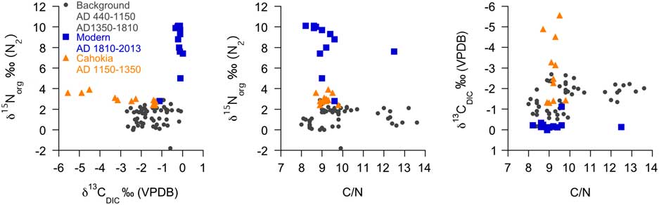
Figure 6. (color online) Scatter plot diagrams of nitrogen isotopes of organic matter (δ15Norg), carbon isotope measurements of carbonate sediment (δ13CDIC), and C/N proxies from Horseshoe Lake. Shifts in δ15Norg are not the result of changes in organic matter source as indicated by C/N ratio. Instead, δ15Norg and C/N suggest that it was likely a change in the source of dissolved nitrogen to the lake rather than the total concentration of N that most strongly affected δ15Norg. This is consistent with groundwater contamination from anthropogenic nitrogen (e.g., sewage). Additionally, the scatter plots show that human-driven environmental change during Cahokia affected δ13CDIC in the lake and not C/N. This indicates that prehistoric human activity more strongly affected the DIC cycle in the lake compared with the source of organic matter. When compared, δ15Norg and δ13CDIC reveal two distinct anthropogenic clusters (i.e. Modern and Cahokia) that fall outside the range of background (or natural) values in the core.
CONCLUSION
This study demonstrates that the sediment deposits in Horseshoe Lake contain a detailed record of environmental change and human disturbance to the surrounding catchment associated with the growth and decline of Cahokia. Prehistoric human impacts are detectable in the proxy records over an approximately 70 year period between AD 1150 ± 50 and 1220 ± 50. The timing of these changes corresponds with population growth in the greater American Bottom region during the Stirling and Moorehead Phases (Milner, Reference Milner1998; Fig. 3). Proxy evidence suggests that waste from high population density, weathering of earthen mounds, and runoff from agricultural fields are the primary drivers of biogeochemical change in the sediment during the occupation of Cahokia. The distinct rise in sorbed Pb, Cu, K, and Al concentrations that occur in the absence of large changes in C/N, organic matter, and magnetic susceptibility suggest that anthropogenic activities enhanced sorbed metal transport to the lake but did not substantially change the bulk composition of the sediment. Sewage from high population densities living around the lake was deposited in midden pits that appear to have contaminated the shallow aquifer feeding Horseshoe Lake. Contamination with sewage enriched the isotopic composition of dissolved nitrogen in groundwater delivered to the lake, resulting in higher δ15Norg deposited in the sediments. The construction of earthen mounds and growth of agriculture likely enhanced the respiration of soil organic matter, adding depleted DIC to groundwater delivered to the lake, resulting in lower δ13CDIC. Finally, the contemporaneous deposition of a fine-grained sediment layer is similar to the Maya Clay layers found in lakes near Maya settlements in Central America; we therefore interpret the “Cahokia Clay” deposit in Horseshoe Lake to be the result of human impact to the watershed, and not the result of flooding. The magnitude of the geochemical changes associated with the growth of Cahokia is smaller than is found in sediments deposited during modern times, yet both fall outside the range of natural variability.
ACKNOWLEDGMENTS
We thank Christopher Purcell, Justin Coughlin, and Robert McDermont for their help in the field. We thank Chanda Bertrand for assistance preparing graphite targets for radiocarbon analysis, John Southon and Guaciarra dos Santos for radiocarbon measurements, William Gilhooly for carbon isotope analysis of carbonate minerals, and David Dettman for the analyses of nitrogen isotopes, carbon, and nitrogen concentrations. We also thank editors Vance Holliday and Lewis Owen and two anonymous reviewers for their thoughtful comments. This research was funded in part by Geological Society of America research grants awarded to Justin Coughlin, with start-up funds to MBA from the University of Pittsburgh and support from the National Science Foundation (EAR-IF 0948366). DPP recognizes support from the Mellon Predoctoral Fellowship from the Dietrich School of Arts and Sciences at the University of Pittsburgh and postdoctoral support at Kansas State University (NSF DEB-1145815) during the preparation of this article.
SUPPLEMENTARY MATERIAL
To view supplementary material for this article, please visit https://doi.org/10.1017/qua.2018.141