


1. Introduction
Shock impingement and large associated changes in local flow-field properties are prevalent for hypersonic flight vehicles (Heiser & Pratt Reference Heiser and Pratt1994; Ward & Smart Reference Ward and Smart2021). While an uncontrolled flow separation results in an engine unstart (Im & Do Reference Im and Do2018) and energy losses, shock impingement in internal flow configurations also initiates combustion (Laurence et al. Reference Laurence, Karl, Schramm and Hannemann2013; Landsberg et al. Reference Landsberg, Wheatley, Smart and Veeraragavan2018; Curran, Wheatley & Smart Reference Curran, Wheatley and Smart2019) and flame-holding (Chang et al. Reference Chang, Park, Jin and Byun2016, Reference Chang, Yang, Park and Choi2018; Landsberg et al. Reference Landsberg, Vanyai, McIntyre and Veeraragavan2020a,Reference Landsberg, Vanyai, McIntyre and Veeraragavanb; Vanyai et al. Reference Vanyai, Landsberg, McIntyre and Veeraragavan2021). Although beneficial, the extreme local thermal loads may also result in structural failure (Stillwell Reference Stillwell1965). The magnitude of flow separation and corresponding thermal loads are highly dependent on the state of the boundary layer. Hence, a number of experiments with simplified canonical models (Dolling Reference Dolling2001; Gaitonde Reference Gaitonde2015; Whalen et al. Reference Whalen, Schöneich, Laurence, Sullivan, Bodony, Freydin, Dowell and Buck2020) have been conducted to further understand the complex flow physics of the impinging shock–boundary layer interaction (SBLI) in different boundary layer states.
Much of the previous experimental work on impinging SBLI focused on low-supersonic flows, demonstrating long test time and offering various options for flow diagnostics. Based on the laminar SBLI experiments of Hakkinen et al. (Reference Hakkinen, Greber, Trilling and Abarbanel1959), Katzer (Reference Katzer1989) conducted an extensive numerical study with a range of Mach numbers from 1 to 3.4 and found that the laminar separation length was linearly dependent on the incident shock strength. The incipient separation was well predicted with the free interaction theory (Chapman, Kuehn & Larson Reference Chapman, Kuehn and Larson1958), which states that the upstream flow properties only dictate the separation process. The good agreement between numerical and experimental works on laminar SBLI has motivated a recent numerical study of Lusher & Sandham (Reference Lusher and Sandham2020). Turbulent SBLIs are still less well understood, as the interactions feature low-frequency modes of shock unsteadiness (Dupont, Haddad & Debiève Reference Dupont, Haddad and Debiève2006; Souverein, Bakker & Dupont Reference Souverein, Bakker and Dupont2013; Clemens & Narayanaswamy Reference Clemens and Narayanaswamy2014; Sasidharan & Duvvuri Reference Sasidharan and Duvvuri2021) and scaling effect of wall heating (Jaunet, Debiève & Dupont Reference Jaunet, Debiève and Dupont2014). Further studies investigated the confinement effects (Grossman & Bruce Reference Grossman and Bruce2018) and the spanwise width of the shock generator (Grossman & Bruce Reference Grossman and Bruce2019) in a three-dimensional duct.
Compared with supersonic wind tunnels, hypersonic facilities manifest a number of challenges in replicating realistic test flows. Many facilities also have short test durations, limiting the options for flow diagnostics and data acquisition. Impulse facilities such as shock/expansion tunnels (Gu & Olivier Reference Gu and Olivier2020) are able to reproduce realistic aerothermal loads of high-Mach-number hypersonic flight. SBLI experiments in impulse facilities (Mallinson, Gai & Mudford Reference Mallinson, Gai and Mudford1996, Reference Mallinson, Gai and Mudford1997; Davis & Sturtevant Reference Davis and Sturtevant2000; Holden et al. Reference Holden, Wadhams, MacLean and Dufrene2013b; Swantek & Austin Reference Swantek and Austin2015; Knisely & Austin Reference Knisely and Austin2016) examined thermochemical non-equilibrium in compression-corner/wedge geometries, in which the total enthalpies typically exceeded 5 MJ kg $^{-1}$. Comprehensive experimental data on the impinging shock configurations in a hypersonic shock tunnel include the studies by Sriram & Jagadeesh (Reference Sriram and Jagadeesh2014, Reference Sriram and Jagadeesh2015) and Sriram et al. (Reference Sriram, Srinath, Devaraj and Jagadeesh2016). Focusing on the large-scale laminar separation bubbles, they developed a linear correlation on separation length and the pressure ratio measured across the shock. The impulse facility further requires a high total pressure (Gildfind et al. Reference Gildfind, Morgan, Jacobs and McGilvray2014) to generate high dynamic pressure test flows for sustained hypersonic flight (Urzay Reference Urzay2018). Owing to the challenges associated with this extra requirement, very few studies report an impinging-shock-flat-plate experiment in high-enthalpy-density hypersonic flows. Sandham et al. (Reference Sandham, Schülein, Wagner, Willems and Steelant2014) observed a weak interaction, where an impinging shock generated by a
  $6^{\circ }$ deflection angle promoted boundary layer transition over a two-dimensional flat plate at Mach 6. Strong interaction data from the LENS shock tunnel is reported in Holden et al. (Reference Holden, Wadhams, MacLean and Dufrene2013a), where an oblique shock is generated by a
  $20^{\circ }$ shock generator which separated the turbulent boundary layer at Mach 11.2. Nonetheless, the high freestream Reynolds number is produced by a low freestream temperature (68 K), which led to ‘cold’ hypersonic data.
While the high Reynolds numbers in the ‘cold’ test flows are suitable for transitional/turbulent studies, this is at the cost of lower static temperature and flow velocity than that of a flight condition. The majority of high-density impinging SBLI data were obtained in these ‘cold’ test flows. Schülein (Reference Schülein2006) conducted a detailed study of closely spaced surface pressure, skin friction and heat-transfer measurements of impinging SBLI in Mach 5 Ludwieg tunnel flows, which have been widely used as validation data for Reynolds-averaged Navier–Stokes (RANS) turbulence models (Brown Reference Brown2013) and direct numerical simulations (Fu et al. Reference Fu, Karp, Bose, Moin and Urzay2018, Reference Fu, Karp, Bose, Moin and Urzay2019, Reference Fu, Karp, Bose, Moin and Urzay2021; Volpiani, Bernardini & Larsson Reference Volpiani, Bernardini and Larsson2020). For strong shock interactions, the reattaching boundary layer downstream could undergo laminar-to-turbulent transition (Schülein Reference Schülein2014; Willems, Gülhan & Steelant Reference Willems, Gülhan and Steelant2015; Currao et al. Reference Currao, Choudhury, Gai, Neely and Buttsworth2020), producing higher heat transfer than purely laminar or turbulent interactions.
There is limited experimental data on impinging SBLI at flight-representative hypersonic conditions in the literature. Therefore, this study aims to fill this gap with detailed surface data from an impinging SBLI experiment conducted in the University of Queensland's T4 Stalker Tube. In line with this, the present authors examined the effect of high wall temperatures in impinging shock-induced flow separation on a heated flat plate (Chang et al. Reference Chang, Chan, Hopkins, McIntyre and Veeraragavan2020, Reference Chang, Chan, McIntyre and Veeraragavan2021). One shortcoming of the hot-wall studies was that the model lacked surface instrumentation due to its high wall temperature. Hence, the quantitative measurement from the unheated, instrumented flat plate in this paper will complement the heated wall data.
2. Methodology
2.1. Test facility and flow conditions
The experimental facility of the present work is the T4 Stalker Tube at the University of Queensland (Stalker et al. Reference Stalker, Paull, Mee, Morgan and Jacobs2005). T4 is a reflected shock tunnel designed to investigate an extensive range of hypersonic flow conditions for scramjet combustion studies (Chan et al. Reference Chan, Razzaqi, Turner, Suraweera and Smart2018b; Landsberg et al. Reference Landsberg, Wheatley, Smart and Veeraragavan2018, Reference Landsberg, Vanyai, McIntyre and Veeraragavan2020a). The facility consists of a reservoir, a compression tube, a shock tube, a nozzle and a test section. The high-pressure air in the reservoir drives the 90.05 kg piston accelerating down the 27 m compression tube. The piston compresses the argon/nitrogen mixture driver gas to high temperature and pressure and ruptures the steel primary diaphragm. The diaphragm rupturing generates a strong shock wave that travels through the 13 m shock tube and reflects at the nozzle-supply region, heating and compressing the test gas (air). The test gas subsequently expands through an axisymmetric Mach 7 nozzle (Chan et al. Reference Chan, Jacobs, Smart, Grieve, Craddock and Doherty2018a). Freestream values were calculated using the ESTCj (Jacobs et al. Reference Jacobs, Gollan, Potter, Zander, Gildfind, Blyton, Chan and Doherty2014) program and are listed in table 1. The first two conditions, labelled as M7A and M7B, simulated Mach 7 flight-equivalent enthalpy and flow speed with 25.9 and 70.3 kPa dynamic pressures, respectively (Chan et al. Reference Chan, Whitside, Smart, Gildfind, Jacobs and Sopek2021). The M7.7B condition produced a Mach 7.7 flight enthalpy with higher temperature and velocity. These three conditions were chosen to investigate the laminar boundary layer prior to shock impingement, with flight-representative freestream Reynolds numbers. Experimental uncertainty for each parameter is estimated using a root-mean-sum method (Mee Reference Mee1993).
Table 1. Facility nozzle-supply (subscript  $s$) and freestream (subscript
  $\infty$) properties.

The measured nozzle-supply (reservoir) pressure is used to determine the available test duration of each flow condition. Typical nozzle-supply pressure traces for all the flow conditions are presented in figure 1. The label  $t$ throughout this paper represents the time since the pressure sensor trigger in the nozzle supply. After the startup period lasting
  $t \approx 1$ ms, steady nozzle-supply pressure is attained until
  $t \approx 5$ ms, 3.5 ms and 3.8 ms for M7A, M7B and M7.7B conditions, respectively. For these low-enthalpy flow conditions, the test duration is terminated by a drop in nozzle-supply pressure. Please note that the correlation developed from the mass spectroscopy measurements in the T4 Stalker Tube (Boyce, Takahashi & Stalker Reference Boyce, Takahashi and Stalker2005) indicates that the driver gas arrival is expected to occur much later than the end of the steady nozzle-supply duration.

Figure 1. Typical nozzle-supply pressure traces for the test conditions listed in table 1. The vertical lines indicate durations at approximate constant nozzle-supply pressure.
Next, the freestream was characterised by the Pitot probe that was located 43 mm away from the centre of the nozzle-exit plane. The Pitot probe's streamwise location was 30 mm, 35 mm or 40 mm upstream of the nozzle-exit plane for the various recoil displacements of the Mach 7 nozzle. The time history of the typical Pitot pressure on the experimental model is illustrated in figure 2(a). After the startup, the Pitot pressure level becomes steady at  $t = 2.0$ ms and is maintained until
  $t = 4.0$ ms. Figure 2(b) shows a good agreement between the measured Pitot pressure and the nozzle simulation, validating the freestream properties. Using the equilibrium nozzle-supply properties calculated by the ESTCj as inputs, the nozzle simulation followed the process outlined in Chan et al. (Reference Chan, Jacobs, Smart, Grieve, Craddock and Doherty2018a). For the experimental pressure, the error bar is given by two times the standard deviation (95 % confidence interval) of the measured signal during the steady test time.

Figure 2. Pitot pressure inspection: (a) time history of M7B Pitot pressure; (b) comparison of the nozzle simulation with the mean pressure.
2.2. Test models and data collection
In this study, we utilised an instrumented flat plate model as shown in figure 3. The labelled  $x$ and
  $y$ directions in the figure are the streamwise and vertical distance from the leading edge of the flat plate, respectively. The leading edge was sharp (
 $r < 0.1$ mm) and replaceable. The flat plate had an axial length (
 $x$) of 626 mm and a spanwise width of 200 mm. With the plate fitting within the Mach 7 nozzle core-flow (Chan et al. Reference Chan, Jacobs, Smart, Grieve, Craddock and Doherty2018a), the surface gauges were placed close to the centreline so that the measurement locations were not affected by the flow spillage and edge effects. There were three streamwise rows of sensors to measure quantitative surface pressure and heat transfer. Two 13 mm-spaced rows (centreline and 13 mm offset) distributed Kulite XTEL-190 (M) piezoresistive pressure sensors from
  $x = 108$ mm to
  $x = 420$ mm. To protect from the harsh test environment, the Kulite sensors were recess-mounted with a hole-diameter of 1.5 mm. Next to the centreline, a single 13.5-mm-spaced row of thin-film heat-transfer gauges (HTGs) were flush-mounted from
  $x = 88.5$ to
  $561$ mm. Below the leading edge, a piezoelectric pressure probe in line with the flat plate was installed to measure the Pitot pressure of the nozzle core flow. The three-dimensionally (3-D) printed shielding protected the instrumentation cabling on the lower side of the plate.

Figure 3. Schematic for the instrumented flat plate and shock generator configurations. All dimensions in millimetres.
Above the flat plate, a 215-mm-long, 172-mm-wide shock generator plate was positioned at  $12^{\circ }$ and
  $16^{\circ }$ deflection to the freestream, producing an inviscid shock strength (
 $\,p_{2}/\,p_{\infty }$) of 5.53 and 8.35, respectively. While the
  $12^{\circ }$ shock generator was positioned at the same location as that of the previous work (Chang et al. Reference Chang, Chan, McIntyre and Veeraragavan2021), the
  $16^{\circ }$ generator was positioned at
  $x = 40$ mm and
  $y = 90$ mm to impinge a shock at a similar location as the 12
 $^{\circ }$ shock generator. Theoretical impingement locations of the
  $12^{\circ }$ and
  $16^{\circ }$ generators at Mach 7 freestream were
  $x \approx 260.4$ mm and
  $x \approx 255.1$ mm, respectively.
Three-dimensional effects can play a significant role in highly separated flows. To minimise these effects, the model was designed to be as large as possible to fit within the Mach 7 nozzle core flow to keep the flow spillage as far away from the measurement locations as possible. We did not put any sidewalls to reduce the spillage because sidewalls were observed to increase the separation length (Holden & Moselle Reference Holden and Moselle1970). The aspect ratio, defined by the ratio between the span of the flat plate and the interaction length (the distance of shock impingement), is a parameter used to check the two-dimensionality. For example, in the Mach 5.8 impinging-shock flat-plate configuration of Currao et al. (Reference Currao, Choudhury, Gai, Neely and Buttsworth2020), the experimental data showed a closer match in separation, peak pressure and heat transfer with the three-dimensional simulation. This highlighted the effect of finite-span with an aspect ratio of  $80/186.6 = 0.43$. In their Mach 2.15 study, Degrez, Boccadoro & Wendt (Reference Degrez, Boccadoro and Wendt1987) found that, if the aspect ratio is larger than 1, the interaction will be two-dimensional. The aspect ratio for our configuration was
  $\approx$0.8. At higher Mach numbers, it is reasonable to expect that two-dimensionality will be better with shallower shock angles. For measuring the separation bubble length, Sriram et al. (Reference Sriram, Srinath, Devaraj and Jagadeesh2016) used a flat plate with a similar aspect ratio (
 $80 / 100 = 0.8$) as our configuration. They used Ball's (Reference Ball1971) conservative estimate of 10
  $\times$ boundary layer thickness at the separation (
 $\delta _{o}$) as a distance from the edges at which three-dimensional effects encroach on the separated flow field. Our maximum
  $\delta _{o}$ is calculated to be 3.2 mm (M7A condition at
  $x = 160$ mm), so the distance is 32 mm. The span of our model is
  $62 \delta _{o}$. Hence, our configuration mostly concerns the two-dimensional core in a separated flow field around the spanwise centre. A three-dimensional RANS computational fluid dynamics (CFD) simulation of the experimental set-up verified that the centreline measurements were indeed in a region where the flow was two-dimensional.
The data acquisition system included 14 National Instruments PXI-6133 cards that produce analogue outputs of all channels at 1 MHz. The system was triggered by the PCB piezoelectric pressure transducers detecting the flow arrival in the nozzle supply. Each Kulite sensor on the instrumented plate was calibrated by taking a two voltage reading from atmosphere and evacuation ( $\approx$40 Pa) for the sensor-specific sensitivity and the offset voltage. Surface heat transfer is measured by the flush-mounted thin-film HTGs. The HTGs used thin (
 $\approx$20 nm) nickel film, which was sputtered onto a quartz substrate to measure the voltage drop (change in resistance due to temperature) from the hypersonic flow. The voltage drop was then converted into heat transfer (
 $q$) by using the process outlined in Schultz & Jones (Reference Schultz and Jones1973), reproduced as
 \begin{equation} q =\frac{\sqrt{{\rho}c{k_{T}}}}{\sqrt{\rm \pi}{\alpha_R} V_{0}}\left[\sum^{j}_{i=1}\frac{V_{(t_0)}- V_{(t_{i-1})}}{\sqrt{t_j-t_i}-\sqrt{t_j-t_{i-1}}}\right].\end{equation}
This equation determines  $q$ by the voltage changes, the product of density
  ${\rho }$, specific heat capacity
  $c$ and thermal conductivity of the nickel
  ${k_{T}}$, and sensor-specific resistivity
  $\alpha _R$. The averaged pressure and heat-transfer values are normalised and presented in § 3. The pressure is normalised by the reading of the upstream sensor at
  $x = 121$ mm. The heat-transfer rate
  $q$ is normalised and presented as the Stanton number (
 $St$). Here
  $St$ is calculated using averaged surface heat transfer
  $q$ from each gauge normalised by the freestream density
  $\rho _{\infty }$, velocity
  $u_{\infty }$, with the difference between nozzle-supply enthalpy
  $H_s$ and air enthalpy
  $h_w$ at
  $T_w = 298$ K:
 \begin{equation} St = \frac{q}{\rho_{\infty}u_{\infty}(H_s-h_w)}.\end{equation}
Using the derived freestream values in table 1 and the uncertainties involved in manufacture and calibration, the uncertainties associated with Stanton number are estimated to be  $\pm$16 %. The measurement uncertainty of pressure is presented by the standard deviation of the mean properties.
The schlieren system was triggered by a TTL signal generated when a pressure signal was detected in the nozzle-supply region (Chang et al. Reference Chang, Chan, Hopkins, McIntyre and Veeraragavan2020). A Phantom v611 high-speed camera captured the flow field at 80 000 and 16 000 frames-per-second with a 0.8  $\mathrm {\mu }$s exposure for the flat plate and shock generator field of view, respectively.
3. Reference data of the flat plate
3.1. Flow establishment and mean surface properties
The initial experiments were conducted without the shock generator to characterise the boundary layer over the flat plate. In addition, the experiments aimed to ensure the flow over the experimental model reached a steady state during the facility's test duration. Typical surface pressure and heat-transfer traces of the flat plate are displayed in figures 4(a) and 4(b), respectively. Both pressure and heat-transfer sensors are exposed to the starting shock passage and produce an initial peak at  $t \approx0.44$ ms. The
  $t$ for this initial peak depends on the streamwise location of the sensor. After the starting shock passage, the test flow arrives and the Mach 7 nozzle requires about 1 ms to start up, indicated by (i) in the figure. With the development of a viscous boundary layer, the pressure and heat transfer reach equilibrium values, requiring about
  $t \approx 1$ ms to establish, labelled as (ii). Then, the pressure becomes steady at around
  $t \approx 2$ ms, and the mean value is taken during (iii). Figure 4(b) also captures temporal heat-transfer traces at two different streamwise locations representing laminar (
 $x = 115.5$ mm) and turbulent (
 $x = 480$ mm) boundary layers. While the laminar heat-transfer signal produces a uniform trace, the fully turbulent signal exhibits a higher magnitude with intense temporal fluctuations. After the test time, the drop of nozzle-supply pressure in figure 1 also results in a decrease of the wall pressure and heat transfer.

Figure 4. Typical surface instrumentation signals during the test, M7B condition: (a) static pressure; (b) heat transfer.
The mean pressure distributions along the plate for M7B and M7.7B condition are plotted in figure 5. The measured pressures were normalised by the sensor at  $x = 121$ mm that produced the smallest standard deviation. Even though the measurement uncertainty of the Kulite sensors is calculated to be 2 %, the standard deviation of the mean pressure level provides a more accurate measure of the temporal variation of the steady pressure levels. Therefore, the error bars are presented by the standard deviation of the respective sensor's mean pressure signal during the steady test time. The standard deviation was also used to determine the error bars in the shock impingement experiment. The pressure levels along the plate do not increase/decrease in the
  $x$ direction, indicating that the flat plate is not angled to the test flow.

Figure 5. Mean static pressure distributions along the flat plate.
Figure 6 shows the mean heat-transfer distribution of the M7B condition. The heat transfer is presented as Stanton number. The plot includes a zoomed inset focusing on the schlieren field of view and temporal heat-transfer plots at multiple  $x$ locations. The theoretical Stanton number distribution calculated using the boundary layer program of Cebeci (Wise & Smart Reference Wise and Smart2014) is also plotted together for comparison. The boundary layer is laminar at
  $x = 264$ mm. At
  $x = 304.5$ mm (
 $Re \approx 1.50 \times 10^{6}$), a turbulent spot is identified by a sharp peak in heat transfer toward the turbulent level in the temporal signals. The heat-transfer pattern agrees with our findings from the heated flat plate (Chang et al. Reference Chang, Chan, Hopkins, McIntyre and Veeraragavan2020), where unstable boundary layer structures were observed at the end of the schlieren field of view. The Stanton number continues to increase. The boundary layer becomes fully turbulent by
  $x = 439.5$ mm, where both the heat-transfer level and the magnitude of the fluctuation are significantly higher than those of the laminar boundary layer. The Reynolds number at this location is
  $2.16 \times 10^{6}$, consistent with the transition Reynolds number of
  $2 \times 10^{6}$ developed from previous flat plate studies in T4 (Mee Reference Mee2002). The heat-transfer measurements from both conditions indicate that the boundary layers are laminar upstream of the expected shock impingement locations (
 $x \approx 260$ mm), confirmed in the heated SBLI work (Chang et al. Reference Chang, Chan, McIntyre and Veeraragavan2021).

Figure 6. Surface heat transfer along the flat plate: M7B condition ( $H_s = 2.37$ MJ kg
 $^{-1}$,
  $Re_{\infty } = 4.92 \times 10^{6}$ m
 $^{-1}$).
The mean Stanton number distribution, schlieren image and heat-transfer signals of various  $x$ locations for the M7.7B condition are displayed in figure 7. The schlieren image shows a uniform boundary layer profile and a laminar heat-transfer level in the field of view. Having a lower Reynolds number than M7B condition, the laminar heat-transfer level of the M7.7B condition sustains until around
  $x = 410$ mm. A turbulent spot is captured at
  $x = 426$ mm (
 $Re \approx 1.34 \times 10^{6}$), characterised by a sharp peak of heat transfer reaching to a fully turbulent level during the steady test time. Moving downstream, the boundary layer undergoes transition with an increase in the frequency of turbulent spots and the mean Stanton number values. At the last measurement point (
 $x = 561$ mm,
  $Re \approx 1.77 \times 10^{6}$) the heat transfer values reach nearly turbulent levels.

Figure 7. Surface heat transfer along the flat plate: M7.7B condition ( $H_s = 2.88$ MJ kg
 $^{-1}$,
  $Re_{\infty } = 3.09 \times 10^{6}$ m
 $^{-1}$).
While both M7B and M7.7B conditions revealed boundary layer transition along the plate, the upstream boundary layer before the shock impingement ( $x_{imp}$ of 252, 255 and 260 mm) remained laminar. This suggests that the shock impingement will likely show laminar separation patterns. The results also showed that the transition of the boundary layer is highly dependent on the Reynolds number. Having much lower Reynolds numbers, the M7A condition produced fully laminar heat-transfer profiles over the plate.
4. Shock impingement tests
4.1. Establishment of the flow separation
The establishment time of the steady separated flow often poses a challenge for the short test duration of impulse facilities. Previous experimental works of flow separation in impulse facilities (Holden Reference Holden1971; Mallinson et al. Reference Mallinson, Gai and Mudford1997; Swantek & Austin Reference Swantek and Austin2015; Knisely & Austin Reference Knisely and Austin2016; Chang et al. Reference Chang, Chan, McIntyre and Veeraragavan2021) observed various characteristic flow lengths depending on the model geometries, using surface measurements and the shock structures from optical visualisations as measures to determine the flow establishment. Our previous work (Chang et al. Reference Chang, Chan, McIntyre and Veeraragavan2021) indicated that the position of the separation shock required the longest time to stabilise, so an in-depth characterisation of the flow establishment was conducted using the schlieren images and surface instrumentation signals recorded during the tests.
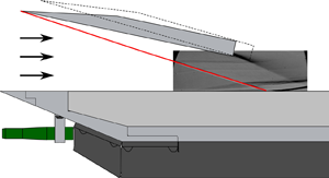
The time evolution of schlieren images of the typical flow field is presented in figure 8. Flow is from left to right for all images. Upon initiation of the test, the test flow appears as shown in figure 8(a), with an oblique shock forming from the top left corner of the image. As the facility nozzle flow starts, the oblique shock is seen to impinge on the flat plate boundary layer is shown in figure 8(b). In addition to the separation shock, shocks from the model leading edge and slight model surface unevenness form. Expansion fans also propagate from the shock generator's trailing edge to downstream of the shock impingement. Because of the expansion, the leading edge shock deflects away from the flat plate. Throughout the test duration, the impinging shock experiences small fluctuations due to the flow fluctuations inherent in shock tunnel flows. As the separation shock moves upstream (figure 8c), the flow recirculation produces a region of low pixel intensity. This recirculation continues to undergo establishment (figure 8c,d) as the pixel intensity increases in figure 8(e). The flow field then reaches steady state when the streamwise position of the separation shock and the recirculation stabilises as shown in figure 8(f,g). The shock also slightly fluctuates at this location due to the unsteadiness in the SBLI and freestream turbulence which is manifested as oscillations in separation. While the laminar boundary layer exhibits distinct white lines (high pixel intensity) due to uniform density gradient, the chaotic flow structures under the reflected shock at  $x \approx 290$ mm qualitatively show that the shock impingement induces boundary layer transition. The evidence of transition was quantitatively verified by the surface heat transfer, which will be further discussed later in this section. After the steady test time, the separation shock gradually moves upstream until the shock front moves outside the field of view (figure 8h).

Figure 8. Time evolution of the M7B, 12 $^{\circ }$ shock generator flow field: (a)
  $t = 0.47$ ms, (b)
  $t = 0.93$ ms, (c)
  $t = 1.60$ ms, (d)
  $t = 2.00$ ms, (e)
  $t = 2.93$ ms, (f)
  $t = 3.67$ ms, (g)
  $t = 3.80$ ms and (h)
  $t = 10.00$ ms.
The wall pressure traces at critical points of the flow field for the M7B, 12 $^{\circ }$ shock generator test are displayed in figure 9. In the figures,
  $t_{st}$ represents the sensor-specific steady test-time duration. The labels (i), (ii) and (iii) represent a division for the flow establishment of the test model in a global time scale. With the flow arrival and passage at respective sensors, the pressure signal in the upstream boundary layer (
 $x = 121$ mm), shown in figure 9(a), exhibits a relatively flat profile, reaching steady state by
  $t \approx 1.5$ ms and sustains until
  $t \approx 4$ ms. The pressure near the onset of separation (
 $x = 179.5$ mm), shown in figure 9(b), provides a direct indication of the behaviour of the separation shock. After the flow arrival at
  $t \approx 0.4$ ms, a highly fluctuating signal occurs until
  $t \approx 2.3$ ms, indicating the stem of the separation shock moves upstream and downstream of the sensor. Then, the pressure gradually recovers to the upstream pressure level (2.7 kPa) from
  $t \approx 3$ ms to
  $t \approx 4$ ms while the separation shock positions downstream of the sensor. The pressure upstream of the impingement (
 $x = 264.5$ mm, figure 9c) shows high levels of fluctuations due to a slight movement of the impinging shock. Therefore, the mean signal of this sensor exhibits a larger standard deviation when averaged through the steady test time (iii). Downstream of the shock impingement, the pressure trace in figure 9(d) is more gentle than that near the impingement. The signal reaches a steady state earlier at
  $t \approx 2$ ms and sustains until
  $t \approx 4$ ms.

Figure 9. Time histories of static pressure for the M7B condition, 12 $^{\circ }$ shock generator: (a)
  $x = 121$ mm, upstream boundary layer; (b)
  $x = 179.5$ mm, onset of separation; (c)
  $x = 264.5$ mm, upstream of shock impingement; (d)
  $x = 309.5$ mm, downstream of shock impingement.
While we can deduce the evolution of macroscopic flow features (e.g. shock and expansion waves) from the pressure measurements, flow separation occurs predominately due to the viscous interaction. Therefore, the temporal evolution of heat transfer ( $\dot {q}$), which is a measure of diffusive phenomena, serves as a more sensitive indicator of flow establishment. Hence, these signals determine the durations for global flow establishment (labels (i), (ii) and (iii)) to calculate the mean values. The heat-transfer signals at the locations close to the pressure sensors are displayed in figure 10. Similar to the pressure sensor at the close location, the heat-transfer signal at the upstream boundary layer (
 $x = 102$ mm, figure 10a) shows a flat profile, reaching a steady state by
  $t \approx$ 1.4 ms and sustains until
  $t \approx 4$ ms. The heat-transfer sensor after the onset of separation (at
  $x = 183$ mm, figure 10b) records a drop in heat transfer due to the separation shock. The separation lifts the boundary layer and yields a zero velocity gradient, which, in turn, leads to a drop in the heat-transfer level throughout. The fluctuations indicate that the steady level sustains only from
  $t \approx 3.1$ ms to
  $t \approx 3.8$ ms (red arrow). Hence, this
  $t_{st}$ is chosen as an averaging window for all pressure and heat-transfer sensors. Note that this is shorter than the
  $t_{st}$ for the pressure signal in the onset of separation (
 $x = 179.5$ mm, figure 9b). The heat-transfer traces upstream (figure 10c) and downstream (figure 10d) of the impingement exhibit very similar characteristics as the pressure traces in the similar locations. With regards to the measurements of the separation, the signals just upstream of impingement (figures 9b,c and 10b,c) exhibit higher fluctuations due to the instabilities in the impinging shock location and flow separation. Interestingly, the signals at a location bounded by the stem and impingement (
 $x = 237.5$ and 244 mm), shown in figure 11(a,b), exhibit steady profiles in pressure during the test time, but high fluctuations in heat transfer with occasional turbulent peaks. This possibly indicates that a mass transfer in the recirculation region promotes boundary layer transition.

Figure 10. Time histories of heat transfer for the M7B, 12 $^{\circ }$: (a)
  $x = 102$ mm, upstream boundary layer; (b)
  $x = 183$ mm, onset of separation; (c)
  $x = 264$ mm, upstream of shock impingement; (d)
  $x = 291$ mm, downstream of shock impingement.

Figure 11. Measured signals inside the separation bubble: (a) pressure,  $x = 244.5$ mm; (b) heat transfer,
  $x = 237$ mm.
To further characterise the separation, the normalised establishment time  $t_{est}$ was determined from heat-transfer signals. Here
  $t_{est}$ was defined by the starting time for
  $t_{st}$ defined previously as steady test duration from the flow arrival divided by the flow residence time (flow length)
  $t_{flow}$. The
  $t_{flow}$ with the streamwise model length of
  $x$, is given by
 \begin{equation} t_{flow} = \frac{x}{u_{\infty}}. \end{equation}
In the present work,  $x = 626$ mm. Another correlation for the normalised establishment time of a laminar boundary layer over a flat plate was empirically developed by Gupta (Reference Gupta1972), which is given by
 \begin{equation} t_{est} = {\frac{1}{0.3}} \times t_{flow}. \end{equation}
 Figure 12 displays the normalised establishment time along the flat plate with the M7B condition. For the gauges measuring the laminar boundary layer,  $t_{est}$ of 3–4
  $t_{flow}$ is needed, matching Gupta's correlation very well. The establishment time on the plate is largest (about 10) near the onset of separation (
 $x = 183$ mm). Then the time gradually decreases along the flow field and requires 5–6
  $t_{flow}$ at the impingement. Downstream of the impingement,
  $t_{est}$ of 4–7
  $t_{flow}$ are required with higher heat flux than the laminar region. This is also observed by the higher fluctuations in the HTGs and the appearance of chaotic, turbulent structures in the schlieren images.

Figure 12. Establishment time comparisons for the impinging shock geometry, M7B condition.
For the impinging shock geometry with the M7B condition, the maximum  $t_{est}$ requires 10 normalised flow times of the experimental model, or 83 flow lengths based on the
  $L_{sep}$ of 80 mm. An expansion tube study by Swantek & Austin (Reference Swantek and Austin2015) also inspected the heat-transfer signals to examine the establishment of separation for a double-wedge model. The
  $t_{est}$ from the test gas arrival was 2 to 8 throughout the flow field. Note that the starting process for the expansion tube involves the passage of the accelerator gas, which assists in the establishment by developing a prior flow before the subsequent test gas (James et al. Reference James, Cullen, Wei, Lewis, Gu, Morgan and McIntyre2018). The establishment times for the impinging shock geometry requires slightly longer than the double-wedge geometry. In addition, the requirement of three flow lengths (Jacobs et al. Reference Jacobs, Rogers, Weidner and Bittner1992) typically used for the experimental models in the T4 facility is not sufficient for these large-scale separated flows. Nonetheless, the separation was established by using the flow conditions with a sufficiently long test-time.
4.2. Mean surface properties of the 12 $^{\circ }$ and 16$^{\circ }$ shock generator


Next, the mean surface properties during the steady test time were examined for all conditions. Figure 13 compares the pressure and Stanton number distributions for the 12 $^{\circ }$, Mach 7 enthalpy (M7A and M7B) flow conditions. The inset of the pressure plot (figure 13a) depicts the onset of separation for the M7B condition at
  $x = 180$ mm. These locations agree well with our previous linear extrapolation of schlieren images to find the stem of the separation shock (Chang et al. Reference Chang, Chan, McIntyre and Veeraragavan2021). The normalised pressure required for onset of separation (
 $\,p_{o}/\,p_{w}$) is 1.55, which is measured when the separated wall pressure reaches a steady level at
  $x = 192.5$ mm. The pressure behind the separation experiences a jump at
  $x \approx 264$ mm, near the inviscid shock impingement location (blue vertical line in the figure). The mean pressure in the vicinity of the impingement produces larger error bars due to the fluctuations of the impinging shock during the steady test time. The normalised pressure stabilises at around
  $21.4 p_w$ at
  $x = 270.5$ mm. The flow then undergoes additional compression to a normalised pressure of 25.5 at
  $x = 303$ mm until the expansion fan from the shock generator trailing edge reaches the plate at
  $x \approx 316$ mm.

Figure 13. Mean properties of the 12 $^{\circ }$ shock generator, M7A and M7B: (a) static pressure and (b) Stanton number. The blue line indicates the inviscid shock impingement point.
Having a lower Reynolds number, the M7A condition produces a pressure distribution (closed square) with a larger separation starting from  $x = 160$ mm. The pressure trend is similar with M7B, except the M7A data follow a very good agreement with the theoretical pressure ratio across the shock (
 $\,p_{3}/\,p_{w}$) calculated by the ideal oblique shock relations. The M7B pressure distribution at this region is slightly higher, possibly due to the higher Reynolds number (
 $Re_{\infty }$) of the M7B condition exhibiting a transitional behaviour, recording higher pressures than the theoretical pressure ratio downstream of the impingement.
Stanton number distributions for the shock generator and the baseline flat plate are detailed in figure 13(b). Top and bottom insets show enlarged views of the heat transfer in upstream boundary layer (before shock interaction) and downstream of the impingement, respectively. As seen in the top inset, the heat transfer upstream of the onset separation is laminar, yet decreases at  $x = 192.5$ mm as the separation shock lifts the boundary layer. Then, significant heating loads are experienced downstream of the impingement, raising the mean Stanton number to
  $10.8 \times 10^{-3}$ at
  $x = 291$ mm. This corresponds to an averaged
  $\dot {q}$ of 2.07 MW m
 $^{-2}$ with a
  $T_{w}$ of 298 K. The M7A condition also produces a similar level of maximum Stanton number (
 $10.1 \times 10^{-3}$) yet much smaller heat-transfer rate of 0.57 MW m
 $^{-2}$ at
  $x = 277.5$ mm. The shock induces an immediate transition to turbulence, and the high heating load sustains until the expansion waves start to diminish the heat transfer at
  $x = 318$ mm. In the bottom inset, the Stanton number maintains turbulent heat-transfer levels up until
  $x \approx 480$ mm. At
  $x = 530$ mm, however, comparison with the flat plate (open symbols in the bottom inset) reveals that the shock-processed boundary layer relaminarises (Willems et al. Reference Willems, Gülhan and Steelant2015), whereas the Stanton number seems to decrease to a lower level than the analytical solution (Cebeci & Bradshaw Reference Cebeci and Bradshaw2012). This is very likely due to the expansion fan emanating from the top of the shock generator (blue cross in figure 3).
A qualitatively similar trend for pressure and heat-transfer distributions is seen in the M7.7B flow field, shown in figure 14. The onset of separation at  $x = 166.5$ mm is depicted in the inset, which is more upstream than that of the M7B case due to a lower
  $Re_{\infty }$. Here,
  $\,p_{o}/\,p_{1}$ is 1.48 at
  $x = 186$ mm. Compared with the M7B result, the normalised pressure downstream of the shock impingement (
 $x = 270.5$ mm) has a smaller value of 18, mainly because of a lower
  $M_{\infty } = 6.85$. Similar to other 12
 $^{\circ }$ shock generator results, the pressure gradually increases until the normalised pressure reaches 22 at
  $x = 303.5$ mm. The maximum Stanton number recorded in the flow field (figure 14b) is
  $11.7 \times 10^{-3}$, converting to an averaged heat-transfer rate on a 298 K wall of 1.95 MW m
 $^{-2}$. The expansion fan reduces both pressure and heat transfer further downstream.

Figure 14. Mean properties of the 12 $^{\circ }$ shock generator, M7.7B: (a) static pressure and (b) Stanton number.
A higher shock strength from the 16 $^{\circ }$ generator leads to a significant increase in wall pressure, heat transfer and separation, as shown in figures 15(a) and 15(b). The onset of separation occurs at
  $x = 167$ mm, reaching to a flat level with a
  $\,p_{o} / \,p_{w}$ of 1.55. This value is very close to the 12
 $^{\circ }$ case, corroborating the free-interaction theory. The pressure sensor readings close to the impingement (
 $x = 257$ to
  $270.5$ mm) experience substantial fluctuations due to a movement of the impinging shock with higher strength. The pressure levels then exhibit a relatively flat profile, similar to the pressure distribution of a fully turbulent studies (Schülein Reference Schülein2006). Within the high-pressure region, the maximum Stanton number of
  $16.8 \times 10^{-3}$ is recorded at
  $x = 280$ mm, converting to the averaged
  $\dot {q}$ with a
  $T_{w}$ of 298 K to be 3.29 MW m
 $^{-2}$. This value is about 53 times more than the heat transfer at the upstream boundary layer (
 $x = 156$ mm). When averaged from
  $x = 270.5$ to
  $300.5$ mm, the heat-transfer rate is 3.17 MW m
 $^{-2}$. In comparison with the 12
 $^{\circ }$ case, the 16
 $^{\circ }$ case forms a shorter streamwise distance between the shock impingement and the expansion fan due to the geometry. The expansion fan relieves the pressure downstream of
  $x \approx 303$ mm. Even though the shock strength from the 16
 $^{\circ }$ generator is much higher than that of the 12
 $^{\circ }$ cases, the boundary layer also relaminarises, as shown in the bottom inset. The results suggest that a higher shock strength accompanies a stronger expansion fan, thereby rapidly diminishing the shock-induced turbulence.

Figure 15. Mean properties of the 16 $^{\circ }$ shock generator, M7B: (a) static pressure and (b) Stanton number.
4.3. Maximum heating
A power relationship between the maximum heat transfer and the pressure ratio in the SBLI was proposed by Back & Cuffel (Reference Back and Cuffel1970) and validated experimentally in the report of Hankey & Holden (Reference Hankey and Holden1975):
 \begin{equation} \left( \frac{q_{w,max}}{q_{w,0}}\right) = \left( {\frac{\,p_{max}}{p_{\infty}}}\right)^{n}.\end{equation}
Here,  $q_{w,max}/q_{w,0}$ is the ratio between the maximum heat transfer and the upstream boundary layer, and
  $\,p_{max} / \,p_{\infty }$ is the pressure ratio across the shock wave. The value
  $n$ was determined as 0.85 or 0.80 for turbulent boundary layers (Back & Cuffel Reference Back and Cuffel1970; Hung & Barnett Reference Hung and Barnett1973; Hankey & Holden Reference Hankey and Holden1975), and 0.70 for laminar boundary layers (Hankey & Holden Reference Hankey and Holden1975). While the
  $n$ values from the literature were based on the separation of either fully laminar or turbulent boundary layers, the present investigation showed an upstream laminar boundary layer transitioning to turbulence by the shock impingement. To correlate the present data with existing correlations,
  $q_{w,0}$ is selected as the heat-transfer rate upstream of the separation. The parameters
  $q_{w,max}$ and
  $\,p_{max}$ were the maximum heat-transfer rate and the pressure measured from the shock impingement, respectively.
Figure 16 presents the relationship between the  $q_{w,max}/q_{w,0}$ and
  $\,p_{max}/\,p_{\infty }$ for the present data, along with the results from other literature on the maximum heating with respect to pressure ratio (Harvey Reference Harvey1968; Hankey & Holden Reference Hankey and Holden1975; Mallinson et al. Reference Mallinson, Gai and Mudford1996; Benay et al. Reference Benay, Chanetz, Mangin and Vandomme2006; Roghelina et al. Reference Roghelina, Olivier, Egorov and Chuvakhov2017). The present data includes all of the 12
 $^{\circ }$ and 16
 $^{\circ }$ results with laminar boundary layers upstream of the impingement, as well as the additional results with a shorter shock generator. In figure 16, all results clearly indicate that peak heating increases with peak pressure ratio across the shock. With a similar range of pressure ratio, however, Mallinson et al. (Reference Mallinson, Gai and Mudford1996), Benay et al. (Reference Benay, Chanetz, Mangin and Vandomme2006) and the present data attained a much higher heating ratio than the fully turbulent correlation (
 $(\,p_{max}/\,p_{\infty })^{0.85}$). The new power-law fit, which is
  $q_{w,max}/q_{w,0} \approx 5.64 (\,p_{max}/p_{\infty })^{0.54}$, produced a much better match for the present data and literature. SBLIs with laminar-to-turbulent transition are known to produce higher peak heat transfer than the fully turbulent boundary layers. The discrepancy indicates the enhanced heat-transfer rate in the laminar-to-turbulent transition from the shock impingement. It is postulated that a higher Reynolds number at the interaction (
 $Re_{i}$) could be the reason for this difference. Benay et al.'s (Reference Benay, Chanetz, Mangin and Vandomme2006) data were based on
  $M_{\infty } = 5$,
  $Re_{i} \approx 22.4 \times 10^{5}$, Mallinson et al.'s (Reference Mallinson, Gai and Mudford1996) data were based on
  $M_{\infty } = 9.1$,
  $Re_{i} = 32.2 \times 10^{5}$ and the present data were based on
  $Re_{i} = 8.1 \times 10^{5}$ to
  $13 \times 10^{5}$; all data exhibited laminar-to-turbulent transition and exceeded fully turbulent heat-transfer ratios. In contrast, the laminar separation data of Harvey (Reference Harvey1968) were based on
  $Re_{i}$ from
  $0.32 \times 10^{4}$ to
  $1.3 \times 10^{5}$, Roghelina et al. (Reference Roghelina, Olivier, Egorov and Chuvakhov2017) from
  $Re_{i} = 4.2 \times 10^{5}$. In addition, the formation of Görtler vortices in the reattachment zone was noted throughout the literature (Simeonides & Hasse Reference Simeonides and Hasse1995; Benay et al. Reference Benay, Chanetz, Mangin and Vandomme2006; Roghelina et al. Reference Roghelina, Olivier, Egorov and Chuvakhov2017; Currao et al. Reference Currao, Choudhury, Gai, Neely and Buttsworth2020), and these vortices were shown to cause a spanwise variation of Stanton number, leading to higher peaks of pressure and heat transfer than fully turbulent interactions. These three-dimensional effects are currently an active area of research, where high-fidelity, three-dimensional numerical computations can be used in future work to detail this. Therefore, further test data, heat-transfer measurements in the spanwise direction and advanced infrared thermography to map the reattachment heating could provide more avenues to improve the correlation.

Figure 16. Maximum heating correlation developed from the present data, along with data from the literature.
5. Remarks on the separation length
From the shock impingement studies on a heated plate (Chang et al. Reference Chang, Chan, McIntyre and Veeraragavan2021), we discovered that the effect of wall temperature follows a different scaling than the existing separation length ( $L_{sep}$) correlations (Katzer Reference Katzer1989; Bleilebens & Olivier Reference Bleilebens and Olivier2006):
 \begin{equation} \frac{L_{sep}}{{\delta_{i}}^{*}} \approx K {\frac{\sqrt{\dfrac{Re_{i}}{C}}}{M_{\infty}^{3}}} \left(\frac{p_r-p_{o}}{p_{\infty}}\right),\quad K \approx 0.95, \quad C=\frac{{\mu_{w}}/{\mu_{\infty}}}{{T_{w}}/ {T_{\infty}}}.\end{equation}
 In our previous work (Chang et al. Reference Chang, Chan, McIntyre and Veeraragavan2021), we used the theoretical oblique shock relations to calculate the onset pressure  $\,p_{o}$ and the reattachment pressure
  $\,p_{r}$ because there were no surface instrumentations on the heated plate. Therefore, the measured pressures of the present experiment could verify and complement the heated plate results. The
  $\,p_{o}$ and
  $\,p_{r}$ for the present data were the mean pressure in the onset of separation and the immediately downstream of the reattachment shock, respectively. Here
  $L_{sep}$ was the measured
  $x$ distance between the onset of separation and the shock impingement and
  $\,p_{o}$ was determined by the sensor location where the pressure gradually increases to the plateau pressure. The location was also checked with the schlieren images. The streamwise resolution between sensors was 6.5 mm, by the two 13-mm-spaced rows with an offset of 6.5 mm; this was sufficient to capture the gradual increase in pressure. Using the free-interaction theory, Katzer (Reference Katzer1989) outlined the equation to calculate theoretical
  $\,p_{o}$ by
 \begin{equation} \frac{p_{o}- p_{\infty}}{p_{\infty}} = \frac{1}{2} \gamma {M_{\infty}}^2 P_{inc} [c_{f_{0}}/ ({M_{\infty}}^{2}-1)^{{1}/{2}}]^{{1}/{2}},\end{equation}
where  $c_{f_{0}}$ is the wall shear stress of the undisturbed flat plate boundary layer at the impingement location and the constant
  $P_{inc}$ is
  $1.57~\sqrt {2}$ by the asymptotic triple-deck calculation of Rizzetta, Burggraf & Jenson (Reference Rizzetta, Burggraf and Jenson1978). From (5.2),
  $\,p_{o}$ values are calculated to be 1.86, 1.55 and 1.66
  $\,p_{w}$ for M7A, M7B and M7.7B conditions with a 12
 $^{\circ }$ shock generator, respectively. The measured plateau pressures reached inside the bubble (at
  $x = 199$ mm) are 1.90, 1.56, and 1.69
  $\,p_{w}$ for the three conditions, which were very close to the theoretical estimates. Hence, the measured pressures were used as
  $\,p_{o}$ for the present work.
Using the measured pressures, the freestream properties in table 1, and the boundary layer properties from the Cebeci program (Wise & Smart Reference Wise and Smart2014), the relationship among scaled separation, temperature ratio and the pressure ratio is plotted in figure 17. The present data (filled rectangle) matches well with the trend found from the heated results (Chang et al. Reference Chang, Chan, McIntyre and Veeraragavan2021), validating the pressure measurements leading to a different separation length scaling  $K \approx 0.95$ from the existing wall temperature correlations. With regards to flow parameters in figure 17, Katzer's (Reference Katzer1989) supersonic scaling was based on
  $M_{\infty }$ from 1.4 to 3.4,
  $\,p_{r}/\,p_{\infty }$ from 1.2 to 1.8 and
  $Re_{i}$ from
  $1 \times 10^{5}$ to
  $6 \times 10^{5}$. Bleilebens & Olivier's (Reference Bleilebens and Olivier2006) hypersonic scaling was based on
  $M_{\infty }$ from 7.1 to 8.1,
  $\,p_{r}/\,p_{\infty }$ from 7.03 to 11.5 and
  $Re_{i}$ from
  $3.3 \times 10^{5}$ to
  $3.8 \times 10^{5}$, similar Mach number and but lower Reynolds number than the present data. The present data have a higher
  $\,p_{r}/\,p_{\infty }$ of 22.1 and 38.3 and
  $Re_{i}$ from
  $8.1 \times 10^{5}$ to
  $13 \times 10^{5}$ (for M7B and M7.7B conditions). When compared with both supersonic and hypersonic scaling, although the separation length
  $L_{sep}$ could become significant for the impinging shock configuration, the higher
  $(\,p_{r}-\,p_{o})/\,p_{\infty }$ and higher
  $Re_{i}$ of the present data yields a smaller
  $K$ value. The comparison suggests that the wall temperature ratio effect in flow separation of impinging shock configurations at hypersonic speeds cannot be easily deduced from previous correlations.

Figure 17. Effect of wall-to-freestream temperature ratio on the scaled separation length.
In addition, Davis & Sturtevant (Reference Davis and Sturtevant2000) derived an  $L_{sep}$ correlation from the hypersonic, high-enthalpy SBLI experiments on a compression ramp. Flow parameters were based on
  $M_{\infty }$ from 4.8 to 9.0,
  $Re_{i}$ from
  $0.57 \times 10^{5}$ to
  $11 \times 10^{5}$ and
  $(\,p_{r}-\,p_{o})/\,p_{\infty }$ up to 15.9. The correlation is based on the triple-deck equation and also includes
  $\,p_{o}$ and a scaling parameter
  $\varLambda _{1}$ that considers wall temperature (unheated model so
  $T_{w}$ is fixed) and real gas effects:
 \begin{equation} \frac{L_{sep}}{x_{1}} \propto \frac{\varLambda_{1}}{\gamma^{3/2}M_{\infty}^3} \left(\frac{\,p_{r}-\,p_{o}}{\,p_{\infty}}\right),\quad \varLambda_{1} = \left(\frac{\mu_w}{\mu^{*}}\right) \left(\frac{T^{*}}{T_{e}}\right) \left(\frac{T_w}{T_{e}}\right)^{1/2}. \end{equation}
 In this equation,  $\gamma$ is the ratio of specific heats and
  $\mu$ is the viscosity ratio. Subscripts * and
  $e$ are the states at the reference temperature (Eckhert Reference Eckhert1955) and the boundary-layer edge, respectively. Figures 18(a) and 18(b) compares the present data (including the heated work of our previous paper) with
  $L_{sep}$ scaling of Davis & Sturtevant (Reference Davis and Sturtevant2000). With regards to
  $(\,p_{r}-\,p_{o})/\,p_{\infty }$, comparison with the literature in figure 18(a) reveals that the present data lie reasonably well with the literature (
 $n$ is a slope of linear fit in log–log coordinate, please refer to Davis & Sturtevant (Reference Davis and Sturtevant2000) for more details), showing a power-law relationship between pressure ratio and
  $L_{sep}$. When comparing against the wall temperature parameter
  $\varLambda _{1}$ (figure 18b), the present data has a higher
  $\varLambda _{1}$ than the literature due to a higher
  $T_{w} / T_{\infty }$ achieved from lower
  $T_{\infty }$ or wall heating. More importantly, the scaled
  $L_{sep}$ with the pressure ratio across the shock is in a power-law relationship with
  $\varLambda _{1}$, obtaining a linear slope of
  $n = 0.36$. This trend further indicates that
  $T_{w} / T_{\infty }$ in figure 17 as a sole parameter is insufficient to represent the wall temperature effects in separation length. Rather, a link with the skin friction of the incoming boundary layer and the scaling from triple-deck theory could provide a more comprehensive understanding.

Figure 18. Relationship between the scaled separation length (Davis & Sturtevant Reference Davis and Sturtevant2000) and flow parameters of the present data: (a) pressure ratio, (b)  $\varLambda _{1}$. Lines represents linear fits and
  $n$ is the slope of each line in log–log coordinates.
6. Conclusions
Experiments for the hypersonic shock impingement on a flat plate at hypersonic flight conditions have been performed in the T4 Stalker Tube. Simultaneous measurements of wall static pressure, heat transfer (presented as Stanton number) and schlieren visualisation characterised the unheated shock impingement flow field. The streamwise heat-transfer distribution captured the boundary layer transition to turbulence with  $Re \approx 2.16 \times 10^{6}$. All conditions considered in this study showed that the upstream boundary layer before the shock impingement stayed laminar.
Quantitative analysis from the surface instrumentation was crucial to confirm the establishment of the impinging SBLI flow field. The schlieren images indicated steady shock waves and expansion fans. Postprocessing of temporal pressure heat-transfer signals also revealed that the flow field was globally steady for  $\approx$700
  $\mathrm {\mu }$s. The present geometry required 3–10 normalised flow establishment times to reach a steady state, with the separation shock taking the longest to stabilise. The establishment times were slightly longer than the times for the compression-corner geometry.
The surface properties reached steady-state SBLI flow field. An initial rise in static pressure and a decrease in heat transfer occurred at the onset separation location. The pressure required for the onset of separation ( $\,p_{o}$) was measured successfully, which was very close to the theory. The impingement incurred a pressure plateau which was typically higher than the theoretical ratio. For a fixed enthalpy, an apparent increase in separation length with lower Reynolds number was observed. Experiments with the 16
 $^{\circ }$ shock generator showed an increase in separation with higher pressure/heat-transfer loads compared with the 12
 $^{\circ }$ cases. The Mach 7 enthalpy,
  $Re = 5.0 \times 10^{6}$ condition produced maximum heat-transfer rates of
  $\approx$1.95 MW m
 $^{-2}$ and
  $\approx$3.29 MW m
 $^{-2}$ from the 12
 $^{\circ }$ and 16
 $^{\circ }$ shock generators, respectively. The Mach 7.7 enthalpy,
  $Re = 3.3 \times 10^{6}$ condition produced localised heat-transfer rates of
  $\approx$1.95 MW m
 $^{-2}$ from the 12
 $^{\circ }$ shock generator. These localised heating loads were sustained until the expansion fan originating from the shock generator's trailing edge relieved the pressure and heat transfer. The heat-transfer distribution further demonstrated a laminar-to-turbulent boundary layer transition following the peak heat transfer.
Lastly, the experimental data correlated with the maximum heating and the scaled separation length. The turbulent transition in the present experiment displayed a much higher heating ratio from the shock compression. The relationship between the heat transfer and pressure ratio was found to follow a different power relationship from the turbulent interaction. In terms of maximum pressure ratio, we found reasonable agreement between the 10 $^{\circ }$ and 12
 $^{\circ }$ results and the linear relationship between the separation and the pressure ratio across the shock. There were some deviations at lower pressure ratios, possibly due to the pressure at the onset of separation. The scaled separation length for the present study followed well with our recent heated wall data regarding wall temperature ratio. Furthermore, comparison with Davis & Sturtevant's (Reference Davis and Sturtevant2000) correlation that includes the scaling from triple-deck theory showed a power-law relationship between wall temperature and separation length, in both heated and unheated hypersonic impinging SBLI. More data points of 16
 $^{\circ }$ case will allow a proper comparison with the existing correlation. Future experiments will aim to utilise focused laser differential interferometry (FLDI) measurements that has been developed (Hopkins et al. Reference Hopkins, Porat, McIntyre, Wheatley and Veeraragavan2021) after the data presented in this paper were collected. This will allow quantification of change in turbulence levels in the post-SBLI region.
Acknowledgements
The authors would like to acknowledge Professor D. Mee for in-depth discussion and helping with the manufacture, calibration and postprocessing for the thin-film HTGs. Special thanks to Dr W. Landsberg for setting up the thin-film apparatus, and Dr K. Damm and Dr D. Curran for the assistance in 3-D simulations. The authors also thank K. Hitchcock for his technical support, and the operators Dr R. Whitside, Dr A. Ward, I. Convery-Brien, R. Ananthapadmanaban and K. Hopkins for operating the T4 Stalker Tube. The first author acknowledges the support from the UQ Research Training Scholarship.
Funding
This work was supported under UQ-National University of Singapore Research Collaboration scheme and the Air Force Office of Science and Research award number FA9550-18-1-0265.
Declaration of interests
The authors report no conflict of interest.


