


1 Introduction
Our current understanding of turbulent boundary layers interacting with solid obstacles have been developed for two limiting conditions: (i) flows impinging on a uniformly distributed array of elements where the array size is large compared with the characteristic large scales of the flow; and (ii) flows impinging on single isolated obstacles, such as a sphere, a cylinder or a bluff body of any shape. The intermediate condition, where turbulent flows interact with a small number of obstacles in an isolated group, has received much less attention. Examples of such flows include atmospheric boundary layers over a forest patch, groups of wind turbines, groups of outstanding buildings in cities, marine turbines in tidal channels, river flows over patchy vegetated beds and marine currents impinging on offshore structures. For these flows, the estimation of drag forces that the flow exerts on the group and the knowledge of the structure of the turbulent wake occurring behind the obstacles are extremely important for the purpose of, e.g., predicting the amount of power that a group of turbines (wind or marine) can generate (Vennell Reference Vennell2010, Reference Vennell2011; Myers & Bhaj Reference Myers and Bhaj2012), estimating carbon dioxide exchange between the forests and the atmosphere (Irvine, Gardiner & Hill Reference Irvine, Gardiner and Hill1997; Cassiani, Katul & Albertson Reference Cassiani, Katul and Albertson2008; Huang, Cassiani & Albertson Reference Huang, Cassiani and Albertson2011) or modelling flood routing in rivers with a patchy vegetation cover (Nepf Reference Nepf, Wolanski and McLusky2011, Reference Nepf2012, and references therein).
The current literature pertaining to this class of flows is mainly focused on the case of arrays of cylinders whose height exceeds the depth of the impinging turbulent boundary layer (Ball, Stansby & Alliston Reference Ball, Stansby and Alliston1996; Nicolle & Eames Reference Nicolle and Eames2011; Chen et al.
Reference Chen, Ortiz, Zong and Nepf2012; Zong & Nepf Reference Zong and Nepf2012; Chang & Constantinescu Reference Chang and Constantinescu2015). In all of these studies, the mean flow around the patch can be considered to be predominantly two-dimensional (2D) as the vorticity in the wake of the cylinders and the array extends along one dominant direction, i.e. along the vertical axis (for brevity, we will refer to these as 2D patches). Within this context, Chen et al. (Reference Chen, Ortiz, Zong and Nepf2012) and Zong & Nepf (Reference Zong and Nepf2012) have investigated flow properties of circular patches of cylinders piercing the free surface of open channel flows (i.e. mimicking patches of emergent vegetation in wetlands). The number of cylinders and the size of the patches were varied extensively and their effects on the flows around and within the patch were investigated by means of visualisation techniques and velocity measurements. The results reported from these studies show that the wake behind a porous obstruction varies strongly with the density of the obstruction. It was observed that downstream of the patch there is a steady wake region where longitudinal velocities were approximately uniform along
 $x$
. This region is then followed by a recovery region where longitudinal velocities begin to increase with increasing
$x$
. This region is then followed by a recovery region where longitudinal velocities begin to increase with increasing
 $x$
. The extent of each region increases with decreasing array density and their development is associated with the strength of the shear layers forming along the sides of the array. Further downstream, provided the patch is dense enough, the two shear layers merge and a flow structure resembling a Von Karman vortex street can eventually be recovered.
$x$
. The extent of each region increases with decreasing array density and their development is associated with the strength of the shear layers forming along the sides of the array. Further downstream, provided the patch is dense enough, the two shear layers merge and a flow structure resembling a Von Karman vortex street can eventually be recovered.
Nicolle & Eames (Reference Nicolle and Eames2011) performed 2D direct numerical simulation (DNS) with a cylinder arrangement similar to that of Zong & Nepf (Reference Zong and Nepf2012). Their simulations were carried out at low Reynolds number (
 $Re_{D}=U_{bulk}D/{\it\nu}=2100$
, characteristic Reynolds number of the patch, where
$Re_{D}=U_{bulk}D/{\it\nu}=2100$
, characteristic Reynolds number of the patch, where
 $U_{bulk}$
is the mean velocity of the flow impinging the patch,
$U_{bulk}$
is the mean velocity of the flow impinging the patch,
 $D$
is the diameter of the patch and
$D$
is the diameter of the patch and
 ${\it\nu}$
is the kinematic viscosity) and present an analysis of the drag forces as well as the wake structure within and behind different arrays. They observed that, depending on the cylinder density, three regimes can be identified: (1) for low densities, each cylinder behaves like an isolated body and the wake of the group is composed of well-identifiable individual wakes; (2) at moderate densities, a steady wake forms behind the array and is stabilised by a bleed flow; (3) at high densities, the patch mimics the behaviour of a solid block both in terms of drag and wake development. The drag coefficient
${\it\nu}$
is the kinematic viscosity) and present an analysis of the drag forces as well as the wake structure within and behind different arrays. They observed that, depending on the cylinder density, three regimes can be identified: (1) for low densities, each cylinder behaves like an isolated body and the wake of the group is composed of well-identifiable individual wakes; (2) at moderate densities, a steady wake forms behind the array and is stabilised by a bleed flow; (3) at high densities, the patch mimics the behaviour of a solid block both in terms of drag and wake development. The drag coefficient
 $C_{D}$
found in these simulations increases with increasing density and converges to the
$C_{D}$
found in these simulations increases with increasing density and converges to the
 $C_{D}$
of a solid cylinder with the same diameter as the patch
$C_{D}$
of a solid cylinder with the same diameter as the patch
 $D$
for higher densities. Moreover, they report that for intermediate densities, the value of
$D$
for higher densities. Moreover, they report that for intermediate densities, the value of
 $C_{D}$
is constant. Similar results can be found in Chang & Constantinescu (Reference Chang and Constantinescu2015), who carried out large eddy simulations (LES) of flows past 2D patches with similar arrangements and impinged by a uniform laminar incoming flow and
$C_{D}$
is constant. Similar results can be found in Chang & Constantinescu (Reference Chang and Constantinescu2015), who carried out large eddy simulations (LES) of flows past 2D patches with similar arrangements and impinged by a uniform laminar incoming flow and
 $Re_{D}=10\,000$
. In contrast to Nicolle & Eames (Reference Nicolle and Eames2011), they did not find a constant region for the
$Re_{D}=10\,000$
. In contrast to Nicolle & Eames (Reference Nicolle and Eames2011), they did not find a constant region for the
 $C_{D}$
at intermediate densities. In fact, the drag coefficient was found to increase monotonically with no intermediate plateau. Notwithstanding this discrepancy, the magnitude of
$C_{D}$
at intermediate densities. In fact, the drag coefficient was found to increase monotonically with no intermediate plateau. Notwithstanding this discrepancy, the magnitude of
 $C_{D}$
they report was comparable with the values obtained in Nicolle & Eames (Reference Nicolle and Eames2011).
$C_{D}$
they report was comparable with the values obtained in Nicolle & Eames (Reference Nicolle and Eames2011).
All of the above-mentioned studies have been confined to 2D patches and there is very little information on the flow and drag characteristics of groups of obstacles that are immersed within boundary layers (for brevity, we will refer to these as 3D patches). Such a configuration is probably encountered more often in engineering applications and the natural environment than its 2D counterpart (wind farms, marine turbines in tidal channels, and vegetated patchy beds are very commonly submerged within a turbulent boundary layer) and, hence, deserves to be investigated in as much detail. The height difference between the boundary layer and the obstacles promotes the formation of an additional shear layer which induces strong 3D features to the mean flow, whose effects on drag and wake development need to be clarified.
In this paper, we present results from an experimental study of flow past 3D patches where thick turbulent boundary layers were generated to impinge on finite circular patches made of circular cylinders. The main aim is to investigate the influence of patch density on the drag and wake properties of the patch. The experiments involve direct drag measurements of the patch and characterisation of the mean flow in the wake using particle image velocimetry (PIV).
The paper is organised into four sections: § 2 describes in detail the experimental set-up; § 3 is dedicated to the presentation of the results; § 4 is devoted to discussion and § 5 to conclusions.

Figure 1. Sketch of the experimental set-up and coordinate system (not to scale).
2 Experimental set-up
Experiments were conducted in an open-circuit wind tunnel at the University of Southampton, whose working section dimensions are 0.9 m
 $\times$
0.6 m
$\times$
0.6 m
 $\times$
4.5 m (i.e. width
$\times$
4.5 m (i.e. width
 $\times$
depth
$\times$
depth
 $\times$
length). The experimental set-up and the coordinate system used herein are shown in figure 1, where
$\times$
length). The experimental set-up and the coordinate system used herein are shown in figure 1, where
 $x$
indicates the streamline direction,
$x$
indicates the streamline direction,
 $y$
is the wall-normal direction and
$y$
is the wall-normal direction and
 $z$
the lateral direction. Here
$z$
the lateral direction. Here
 $U$
,
$U$
,
 $V$
and
$V$
and
 $W$
are the mean components of the velocity along these directions, respectively. The origin is located at the centre of the patch.
$W$
are the mean components of the velocity along these directions, respectively. The origin is located at the centre of the patch.
The turbulent boundary layer was generated with a combination of spires and different types of roughness elements of decreasing size. The free-stream velocity of the wind tunnel (
 $U_{\infty }$
), which was set to
$U_{\infty }$
), which was set to
 $20~\text{m}~\text{s}^{-1}$
, was acquired using a Pitot-static tube connected to a Furness FC-012 micromanometer. The boundary layer measurements were taken using a single hot-wire probe (overheat ratio 1.7) driven by a Newcastle (NSW) CTA bridge and acquired by a NI USB-6251 BNC data acquisition system from National Instruments at
$20~\text{m}~\text{s}^{-1}$
, was acquired using a Pitot-static tube connected to a Furness FC-012 micromanometer. The boundary layer measurements were taken using a single hot-wire probe (overheat ratio 1.7) driven by a Newcastle (NSW) CTA bridge and acquired by a NI USB-6251 BNC data acquisition system from National Instruments at
 $x=0$
(patch not present, measurements taken at the location where the patch will be positioned). Calibrations were performed against the Pitot-static tube and all of the data were digitised and analysed using a desktop computer and Matlab software. The hot-wire probe was mounted on a traverse system driven by the same computer and, at each vertical location, measurements were carried out with a sampling frequency of 20 kHz for 2 min. Ambient temperature and pressure were also monitored in order to accurately determine the air density and kinematic viscosity.
$x=0$
(patch not present, measurements taken at the location where the patch will be positioned). Calibrations were performed against the Pitot-static tube and all of the data were digitised and analysed using a desktop computer and Matlab software. The hot-wire probe was mounted on a traverse system driven by the same computer and, at each vertical location, measurements were carried out with a sampling frequency of 20 kHz for 2 min. Ambient temperature and pressure were also monitored in order to accurately determine the air density and kinematic viscosity.

Figure 2. (a) Boundary layer velocity profile:
 $U/U_{\infty }$
versus
$U/U_{\infty }$
versus
 $y/D$
, left-bottom axis,
$y/D$
, left-bottom axis,
 $U_{\infty }$
is the free-stream velocity,
$U_{\infty }$
is the free-stream velocity,
 $D$
is the patch diameter, inner scaling
$D$
is the patch diameter, inner scaling
 $U/u_{{\it\tau}}$
versus
$U/u_{{\it\tau}}$
versus
 $y/y_{0}$
right-top axis,
$y/y_{0}$
right-top axis,
 $u_{{\it\tau}}$
is the friction velocity,
$u_{{\it\tau}}$
is the friction velocity,
 $y_{0}$
is the equivalent roughness length; the log law is represented as a straight line,
$y_{0}$
is the equivalent roughness length; the log law is represented as a straight line,
 $U^{+}=U/u_{{\it\tau}}$
. (b) Standard deviation profile:
$U^{+}=U/u_{{\it\tau}}$
. (b) Standard deviation profile:
 ${\it\sigma}_{U}/U_{\infty }$
versus
${\it\sigma}_{U}/U_{\infty }$
versus
 $y/D$
, left-bottom axis,
$y/D$
, left-bottom axis,
 ${\it\sigma}_{U}/u_{{\it\tau}}$
versus
${\it\sigma}_{U}/u_{{\it\tau}}$
versus
 $y/y_{0}$
right-top axis. Measurements were taken by removing the patch at
$y/y_{0}$
right-top axis. Measurements were taken by removing the patch at
 $x=0$
.
$x=0$
.
The velocity profile of the turbulent boundary layer and the corresponding turbulent fluctuations are shown in figure 2 (
 ${\it\sigma}_{U}$
is the standard deviation of the longitudinal velocity component). All of the main parameters describing the boundary layer are given in table 1, where
${\it\sigma}_{U}$
is the standard deviation of the longitudinal velocity component). All of the main parameters describing the boundary layer are given in table 1, where
 ${\it\delta}$
is the boundary layer thickness here defined as the location where the velocity reaches the 99 % of the free-stream velocity,
${\it\delta}$
is the boundary layer thickness here defined as the location where the velocity reaches the 99 % of the free-stream velocity,
 ${\it\delta}_{\ast }$
is the displacement thickness (
${\it\delta}_{\ast }$
is the displacement thickness (
 ${\it\delta}_{\ast }=\int _{0}^{\infty }(1-(U(y)/U_{\infty }))\,\text{d}y$
) and
${\it\delta}_{\ast }=\int _{0}^{\infty }(1-(U(y)/U_{\infty }))\,\text{d}y$
) and
 ${\it\theta}$
is the momentum thickness (
${\it\theta}$
is the momentum thickness (
 ${\it\theta}=\int _{0}^{\infty }(U(y)/U_{\infty })(1-(U(y)/U_{\infty }))\,\text{d}y$
). The eddy turnover time is estimated as
${\it\theta}=\int _{0}^{\infty }(U(y)/U_{\infty })(1-(U(y)/U_{\infty }))\,\text{d}y$
). The eddy turnover time is estimated as
 ${\it\delta}/U_{\infty }$
and is equal to 0.018 s, which is resolved more than 6500 times within the time span of data acquisition (i.e. 2 min). The size of the hot-wire normalised by the viscous length scale, i.e.
${\it\delta}/U_{\infty }$
and is equal to 0.018 s, which is resolved more than 6500 times within the time span of data acquisition (i.e. 2 min). The size of the hot-wire normalised by the viscous length scale, i.e.
 $l^{+}=lu_{{\it\tau}}/{\it\nu}$
, is equal to 107 (where
$l^{+}=lu_{{\it\tau}}/{\it\nu}$
, is equal to 107 (where
 $u_{{\it\tau}}=\sqrt{{\it\tau}_{w}/{\it\rho}}$
is the friction velocity,
$u_{{\it\tau}}=\sqrt{{\it\tau}_{w}/{\it\rho}}$
is the friction velocity,
 ${\it\tau}_{w}$
is the wall shear stress,
${\it\tau}_{w}$
is the wall shear stress,
 ${\it\rho}$
is the fluid density,
${\it\rho}$
is the fluid density,
 $l$
is the wire length and
$l$
is the wire length and
 ${\it\nu}$
is the air kinematic viscosity). The mean velocity profile exhibited a logarithmic region within the range
${\it\nu}$
is the air kinematic viscosity). The mean velocity profile exhibited a logarithmic region within the range
 $0.7<y/D<1.5$
. Within this region the mean velocity profile can be reasonably approximated by the classical log law of the wall,
$0.7<y/D<1.5$
. Within this region the mean velocity profile can be reasonably approximated by the classical log law of the wall,
 $U/u_{{\it\tau}}={\it\kappa}^{-1}\ln (y/y_{0})$
, where
$U/u_{{\it\tau}}={\it\kappa}^{-1}\ln (y/y_{0})$
, where
 ${\it\kappa}$
is the von Karman constant here taken as 0.41 and
${\it\kappa}$
is the von Karman constant here taken as 0.41 and
 $y_{0}$
is the equivalent roughness length. The friction velocity and the roughness length were estimated by fitting the experimental data with the log law of the wall and using a modified Clauser method, as proposed by Perry & Li (Reference Perry and Li1990) and described also by Flack, Schultz & Shapiro (Reference Flack, Schultz and Shapiro2005) and Flack, Schultz & Connelly (Reference Flack, Schultz and Connelly2007), among others. All of these diagnostic parameters were obtained by averaging data from five different velocity profiles, taken at
$y_{0}$
is the equivalent roughness length. The friction velocity and the roughness length were estimated by fitting the experimental data with the log law of the wall and using a modified Clauser method, as proposed by Perry & Li (Reference Perry and Li1990) and described also by Flack, Schultz & Shapiro (Reference Flack, Schultz and Shapiro2005) and Flack, Schultz & Connelly (Reference Flack, Schultz and Connelly2007), among others. All of these diagnostic parameters were obtained by averaging data from five different velocity profiles, taken at
 $z=0,\pm 25,\pm 50$
and hence representative of the flow impinging the patches.
$z=0,\pm 25,\pm 50$
and hence representative of the flow impinging the patches.

Figure 3. Plane view of the patches and the solid case. The distributions of the cylinders within the patches are the actual configurations used for the measurements and
 $d/D$
is at the right scale.
$d/D$
is at the right scale.
Table 1. Main parameters characterising the incoming boundary layer at
 $x=0$
(patch not present, measurements taken at the location where the patch will be positioned):
$x=0$
(patch not present, measurements taken at the location where the patch will be positioned):
 ${\it\delta}$
is the boundary layer thickness (location where the velocity reaches the 99 % of the free-stream velocity);
${\it\delta}$
is the boundary layer thickness (location where the velocity reaches the 99 % of the free-stream velocity);
 $u_{{\it\tau}}=\sqrt{{\it\tau}_{w}/{\it\rho}}$
is the friction velocity (where
$u_{{\it\tau}}=\sqrt{{\it\tau}_{w}/{\it\rho}}$
is the friction velocity (where
 ${\it\tau}_{w}$
is the wall shear stress and
${\it\tau}_{w}$
is the wall shear stress and
 ${\it\rho}$
is the fluid density);
${\it\rho}$
is the fluid density);
 $y_{0}$
is the equivalent roughness length;
$y_{0}$
is the equivalent roughness length;
 $U_{\infty }$
is the free-stream velocity;
$U_{\infty }$
is the free-stream velocity;
 ${\it\delta}_{\ast }$
is the displacement thickness (i.e.
${\it\delta}_{\ast }$
is the displacement thickness (i.e.
 ${\it\delta}_{\ast }=\int _{0}^{\infty }(1-(U(y)/U_{\infty }))\,\text{d}y$
);
${\it\delta}_{\ast }=\int _{0}^{\infty }(1-(U(y)/U_{\infty }))\,\text{d}y$
);
 ${\it\theta}$
is the momentum thickness (i.e.
${\it\theta}$
is the momentum thickness (i.e.
 ${\it\theta}=\int _{0}^{\infty }(U(y)/U_{\infty })(1-(U(y)/U_{\infty }))\,\text{d}y$
);
${\it\theta}=\int _{0}^{\infty }(U(y)/U_{\infty })(1-(U(y)/U_{\infty }))\,\text{d}y$
);
 $Re_{{\it\theta}}=U_{\infty }{\it\theta}/{\it\nu}$
is the Reynolds number based on the momentum thickness (
$Re_{{\it\theta}}=U_{\infty }{\it\theta}/{\it\nu}$
is the Reynolds number based on the momentum thickness (
 ${\it\nu}$
is the fluid kinematic viscosity).
${\it\nu}$
is the fluid kinematic viscosity).
Circular patches made of circular cylinders with different plan densities (see figure 3) were placed in the centreline of the wind tunnel. The circular patch geometry and its cylindrical constituents were chosen in order to remain consistent with previous studies and hence to enable us to delineate the differences between flows impinging 2D and 3D patches. Moreover, the aerodynamic characteristics of finite-height solid cylinders with circular cross-section are well known (see, e.g., Sumner Reference Sumner2013). This wealth of knowledge provides a solid benchmark for the flow and drag characterisation of the limiting case investigated in this study (i.e. the case where the density is 1) and for the individual constituents of the porous patches.
The solid cylinder case (i.e.
 $C_{S}$
) was made of non-porous polyurethane foam, with a diameter
$C_{S}$
) was made of non-porous polyurethane foam, with a diameter
 $D$
equal to 100 mm and a height
$D$
equal to 100 mm and a height
 $H$
of 100 mm, resulting in an aspect ratio
$H$
of 100 mm, resulting in an aspect ratio
 $AR=H/D$
of 1. The porous patches were realised with 7, 20, 39, 64 and 95 (i.e.
$AR=H/D$
of 1. The porous patches were realised with 7, 20, 39, 64 and 95 (i.e.
 $N_{c}$
) small cylinders (each having a diameter
$N_{c}$
) small cylinders (each having a diameter
 $d=5$
mm and height
$d=5$
mm and height
 $H=100$
mm, corresponding to
$H=100$
mm, corresponding to
 $AR=20$
for each individual cylinder) contained within a patch of diameter
$AR=20$
for each individual cylinder) contained within a patch of diameter
 $D=100$
mm, giving a ratio
$D=100$
mm, giving a ratio
 $D/d=20$
. Following Nicolle & Eames (Reference Nicolle and Eames2011), the cylinders were arranged in concentric circles with one cylinder at the centre of the patch. The spacing between each circle and between each cylinder on the circle was kept the same. The patches were manufactured using 3D printers and figure 3 shows the naming convention that will be used hereafter in this paper. The characteristics of each patch are reported in table 2 and a picture of the
$D/d=20$
. Following Nicolle & Eames (Reference Nicolle and Eames2011), the cylinders were arranged in concentric circles with one cylinder at the centre of the patch. The spacing between each circle and between each cylinder on the circle was kept the same. The patches were manufactured using 3D printers and figure 3 shows the naming convention that will be used hereafter in this paper. The characteristics of each patch are reported in table 2 and a picture of the
 $C_{95}$
patch in the wind tunnel set-up is shown in figure 4(a). The density
$C_{95}$
patch in the wind tunnel set-up is shown in figure 4(a). The density
 ${\it\phi}$
is defined as the ratio of the plane area occupied by all of the individual cylinders within the patch,
${\it\phi}$
is defined as the ratio of the plane area occupied by all of the individual cylinders within the patch,
 $N_{c}{\rm\pi}d^{2}/4$
, and the base area of the patch,
$N_{c}{\rm\pi}d^{2}/4$
, and the base area of the patch,
 ${\rm\pi}D^{2}/4$
(
${\rm\pi}D^{2}/4$
(
 ${\it\phi}=d^{2}N_{c}/D^{2}$
).
${\it\phi}=d^{2}N_{c}/D^{2}$
).
Table 2. Patch characteristics:
 $N_{c}$
is the number of cylinders;
$N_{c}$
is the number of cylinders;
 ${\it\phi}$
is the density (
${\it\phi}$
is the density (
 $d^{2}N_{c}/D^{2}$
,
$d^{2}N_{c}/D^{2}$
,
 $D$
is the diameter of the patch,
$D$
is the diameter of the patch,
 $d$
is the diameter of the individual cylinder). Measurements results for each patch:
$d$
is the diameter of the individual cylinder). Measurements results for each patch:
 $C_{D}$
is the drag coefficient defined by (2.1) for
$C_{D}$
is the drag coefficient defined by (2.1) for
 $U_{\infty }$
of
$U_{\infty }$
of
 $20~\text{m}~\text{s}^{-1}$
;
$20~\text{m}~\text{s}^{-1}$
;
 $C_{Dbulk}$
is the drag coefficient defined by (3.1);
$C_{Dbulk}$
is the drag coefficient defined by (3.1);
 $L_{r}$
is the length of the recovery region along
$L_{r}$
is the length of the recovery region along
 $x$
non-dimensionalised with
$x$
non-dimensionalised with
 $D$
;
$D$
;
 $U_{\infty }$
is the free-stream velocity;
$U_{\infty }$
is the free-stream velocity;
 $U_{bTE}$
is the mean streamwise bleeding velocity at the trailing edge (
$U_{bTE}$
is the mean streamwise bleeding velocity at the trailing edge (
 $x/D=0.52$
);
$x/D=0.52$
);
 $V_{bTE}$
is the mean vertical bleeding velocity at the trailing edge (
$V_{bTE}$
is the mean vertical bleeding velocity at the trailing edge (
 $x/D=0.52$
);
$x/D=0.52$
);
 $x_{rb}$
is the streamwise coordinate of the centre of the recirculation bubble;
$x_{rb}$
is the streamwise coordinate of the centre of the recirculation bubble;
 ${\it\omega}_{zMAX}D/U_{\infty }$
is the minimum value of the top shear layer vorticity at
${\it\omega}_{zMAX}D/U_{\infty }$
is the minimum value of the top shear layer vorticity at
 $x/D=0.75$
and its vertical coordinate
$x/D=0.75$
and its vertical coordinate
 $y_{{\it\omega}_{zMAX}}$
;
$y_{{\it\omega}_{zMAX}}$
;
 ${\it\omega}_{yMAX}D/U_{\infty }$
is the maximum value of the lateral shear layer vorticity at
${\it\omega}_{yMAX}D/U_{\infty }$
is the maximum value of the lateral shear layer vorticity at
 $x/D=0.75$
.
$x/D=0.75$
.

The mean drag force experienced by the patches was measured using a single point load cell (Vishay, model 1004, 600 g) positioned underneath them, and aligned with the flow. The signal from the load cell was acquired using a NI USB-6251 BNC data acquisition system at 20 kHz for 3 min for each case. A picture of the load cell is shown in figure 4(b). The patches were mounted on a plate, which was then connected to the load cell. The base of the patch was flush-mounted with the wind tunnel floor, leaving a clearance around the edges of about 2 mm. This gap allowed for patch movements required for drag measurements. Since the wind tunnel was a suction-type, care was taken to ensure that the whole system was sealed from the external environment, in order to prevent any airflow through the gaps. This was achieved by enclosing the whole drag-measurement system in a PVC box, sealed at the junction with the tunnel. Before every experiment, a thorough calibration of the load cell was performed by loading the system with known calibration weights using a pulley system connected to the model. A sketch of the load cell set-up and the calibration system is shown in figure 5(a). The calibration curve obtained from all of the calibration experiments is shown in figure 5(b). The deviations from the fitting provide an indication of the measurements accuracy and was used to estimate the error
 ${\it\epsilon}_{F_{D}}$
on the force values.
${\it\epsilon}_{F_{D}}$
on the force values.
For each patch, drag measurements were obtained at four different free-stream velocities (10, 15, 20 and
 $25~\text{m}~\text{s}^{-1}$
) and each test was repeated multiple times to ensure repeatability. The drag coefficient was then calculated as
$25~\text{m}~\text{s}^{-1}$
) and each test was repeated multiple times to ensure repeatability. The drag coefficient was then calculated as
 $$\begin{eqnarray}C_{D}=\frac{F_{D}}{1/2{\it\rho}U_{\infty }^{2}DH},\end{eqnarray}$$
where
 $F_{D}$
is the measured average drag force,
$F_{D}$
is the measured average drag force,
 ${\it\rho}$
is the air density and
${\it\rho}$
is the air density and
 $U_{\infty }$
is the free-stream velocity, and averaged within all of the repetitions. The uncertainty on the drag coefficient due to experimental errors associated with all of the independent variables in (2.1) was evaluated using the standard error propagation theory as
$U_{\infty }$
is the free-stream velocity, and averaged within all of the repetitions. The uncertainty on the drag coefficient due to experimental errors associated with all of the independent variables in (2.1) was evaluated using the standard error propagation theory as
 $$\begin{eqnarray}\frac{{\it\epsilon}_{C_{D}}}{C_{D}}=\sqrt{\left(\frac{{\it\epsilon}_{F_{D}}}{F_{D}}\right)^{2}+\left(2\frac{{\it\epsilon}_{U_{\infty }}}{U_{\infty }}\right)^{2}},\end{eqnarray}$$
where
 ${\it\epsilon}_{A}$
represents the error on the generic quantity
${\it\epsilon}_{A}$
represents the error on the generic quantity
 $A$
. The uncertainty on
$A$
. The uncertainty on
 $F_{D}$
is given by the combination of root-mean-square (r.m.s.) error on the calibration, equal to
$F_{D}$
is given by the combination of root-mean-square (r.m.s.) error on the calibration, equal to
 $\pm 1.35$
g, and considering the presence of an offset for each measurement due to electric interference of
$\pm 1.35$
g, and considering the presence of an offset for each measurement due to electric interference of
 $-2.51\pm 0.54$
g. The uncertainty on
$-2.51\pm 0.54$
g. The uncertainty on
 $U_{\infty }$
is given by the r.m.s. of the differences between the velocity on each run and the average velocity of the repetitions. The uncertainties on
$U_{\infty }$
is given by the r.m.s. of the differences between the velocity on each run and the average velocity of the repetitions. The uncertainties on
 ${\it\rho}$
,
${\it\rho}$
,
 $D$
and
$D$
and
 $H$
(
$H$
(
 $\pm$
0.25 mm for 100 mm) were neglected because they were much smaller than those of the variables included in (2.2). The total error on the drag coefficient was evaluated as
$\pm$
0.25 mm for 100 mm) were neglected because they were much smaller than those of the variables included in (2.2). The total error on the drag coefficient was evaluated as
 $$\begin{eqnarray}{\it\epsilon}_{C_{DTOT}}={\it\epsilon}_{C_{D}}+{\it\epsilon}_{C_{D}rms},\end{eqnarray}$$
where
 ${\it\epsilon}_{C_{D}rms}$
accounts for the repetition error due to other unknown sources which are accounted for by repeating the measurements multiple times.
${\it\epsilon}_{C_{D}rms}$
accounts for the repetition error due to other unknown sources which are accounted for by repeating the measurements multiple times.

Figure 4. (a) Picture of the model
 $C_{95}$
in the wind tunnel. (b) Picture of the load cell.
$C_{95}$
in the wind tunnel. (b) Picture of the load cell.

Figure 5. (a) Sketch of the load cell mounting set-up and calibration system. (b) Load cell calibration curve.
PIV measurements were carried out along two different planes, the streamwise–spanwise (
 $x$
–
$x$
–
 $z$
) plane in the wake of the patches at the vertical mid-plane (50 mm from the wall and the top of the patch) and the streamwise–wall-normal (
$z$
) plane in the wake of the patches at the vertical mid-plane (50 mm from the wall and the top of the patch) and the streamwise–wall-normal (
 $x$
–
$x$
–
 $y$
) plane at the centreline of the patches (namely at
$y$
) plane at the centreline of the patches (namely at
 $y=0$
). The PIV measurements were only carried out at a free-stream velocity of
$y=0$
). The PIV measurements were only carried out at a free-stream velocity of
 $20~\text{m}~\text{s}^{-1}$
. Lightsheets were generated by two pulsed Nd:YAG lasers (Nano L200 15PIV, from Litron Lasers) while the images were acquired using three 16MP CCD cameras (LaVision Imager Pro LX CCD, resolution of 4872
$20~\text{m}~\text{s}^{-1}$
. Lightsheets were generated by two pulsed Nd:YAG lasers (Nano L200 15PIV, from Litron Lasers) while the images were acquired using three 16MP CCD cameras (LaVision Imager Pro LX CCD, resolution of 4872
 $\times$
3248 pixels). The lasers and the cameras were controlled and synchronised using DaVis software (v8.2.2) from LaVision. The seeding was generated by means of a smoke machine that produces aerosol particles from a solution of glycol and demineralised water. A total of 3000 pairs of images for all three cameras in both sets of measurements was acquired for each patch at a rate of 0.375 Hz for a total time of about 135 min. For the
$\times$
3248 pixels). The lasers and the cameras were controlled and synchronised using DaVis software (v8.2.2) from LaVision. The seeding was generated by means of a smoke machine that produces aerosol particles from a solution of glycol and demineralised water. A total of 3000 pairs of images for all three cameras in both sets of measurements was acquired for each patch at a rate of 0.375 Hz for a total time of about 135 min. For the
 $x$
–
$x$
–
 $z$
plane measurements, cameras were fitted with 50 mm Nikkor lenses, and the resulting resolution was about
$z$
plane measurements, cameras were fitted with 50 mm Nikkor lenses, and the resulting resolution was about
 $12~\text{px}~\text{mm}^{-1}$
. The time-separation between laser pulses for these measurements was set to
$12~\text{px}~\text{mm}^{-1}$
. The time-separation between laser pulses for these measurements was set to
 $100~{\rm\mu}\text{s}$
. For the vertical
$100~{\rm\mu}\text{s}$
. For the vertical
 $x$
–
$x$
–
 $y$
plane at the centreline of the obstacles (
$y$
plane at the centreline of the obstacles (
 $z=0$
mm), the cameras were fitted with 105 mm Nikkor lenses, resulting in a resolution of about
$z=0$
mm), the cameras were fitted with 105 mm Nikkor lenses, resulting in a resolution of about
 $17~\text{px}~\text{mm}^{-1}$
. The laser pulse separation in this case was set to
$17~\text{px}~\text{mm}^{-1}$
. The laser pulse separation in this case was set to
 $50~{\rm\mu}\text{s}$
. In both cases the acquired data were processed using the graphical processing unit (GPU) version of the DaVis software with a final interrogation window of 16
$50~{\rm\mu}\text{s}$
. In both cases the acquired data were processed using the graphical processing unit (GPU) version of the DaVis software with a final interrogation window of 16
 $\times$
16 pixels with a 50 % overlap. For both cases, the number of acquired images was large enough to reach statistical convergence for first- and second-order velocity statistics. For the solid cylinder case, the vertical plane data show a grey region immediately downstream of the cylinder, due to the shadow cast by the top of the cylinder.
$\times$
16 pixels with a 50 % overlap. For both cases, the number of acquired images was large enough to reach statistical convergence for first- and second-order velocity statistics. For the solid cylinder case, the vertical plane data show a grey region immediately downstream of the cylinder, due to the shadow cast by the top of the cylinder.
3 Results
3.1 Drag measurements
Figure 6 shows the variation of the drag coefficient,
 $C_{D}$
, with Reynolds number,
$C_{D}$
, with Reynolds number,
 $Re_{D}=U_{\infty }D/{\it\nu}$
, for all of the patches. It can clearly be seen that the influence of
$Re_{D}=U_{\infty }D/{\it\nu}$
, for all of the patches. It can clearly be seen that the influence of
 $Re$
on
$Re$
on
 $C_{D}$
is negligible, presumably because of the high level of turbulence characterising the incoming turbulent boundary layer. Therefore, in all subsequent results, we only present the data pertaining to
$C_{D}$
is negligible, presumably because of the high level of turbulence characterising the incoming turbulent boundary layer. Therefore, in all subsequent results, we only present the data pertaining to
 $U_{\infty }=20~\text{m}~\text{s}^{-1}$
(
$U_{\infty }=20~\text{m}~\text{s}^{-1}$
(
 $Re_{D}\simeq 1.1\times 10^{5}$
) since the PIV measurements were carried out at this free-stream velocity.
$Re_{D}\simeq 1.1\times 10^{5}$
) since the PIV measurements were carried out at this free-stream velocity.

Figure 6. Drag coefficient variation with Reynolds number (
 $Re=U_{\infty }D/{\it\nu}$
) for all the patches: ●
$Re=U_{\infty }D/{\it\nu}$
) for all the patches: ●
 $C_{7}$
, ♦
$C_{7}$
, ♦
 $C_{20}$
, ▴
$C_{20}$
, ▴
 $C_{39}$
, ▪
$C_{39}$
, ▪
 $C_{64}$
, ▾
$C_{64}$
, ▾
 $C_{95}$
, ◂
$C_{95}$
, ◂
 $C_{S}$
.
$C_{S}$
.

Figure 7. Drag coefficient variation with patches density non-dimensionalised with
 $U_{\infty }$
versus patches density for
$U_{\infty }$
versus patches density for
 $U_{\infty }=20~\text{m}~\text{s}^{-1}$
. The exact values are reported in table 2.
$U_{\infty }=20~\text{m}~\text{s}^{-1}$
. The exact values are reported in table 2.
Figure 7 shows the variation of
 $C_{D}$
with density (see table 2 for correspondence between
$C_{D}$
with density (see table 2 for correspondence between
 ${\it\phi}$
and patch name and for the actual values). It can be seen that
${\it\phi}$
and patch name and for the actual values). It can be seen that
 $C_{D}$
increases with increasing
$C_{D}$
increases with increasing
 ${\it\phi}$
and seems to converge to a value of about 0.37, which, however, does not correspond to the drag coefficient of the solid case, which is much lower. Surprisingly, the drag coefficient of the solid patch is rather comparable to the
${\it\phi}$
and seems to converge to a value of about 0.37, which, however, does not correspond to the drag coefficient of the solid case, which is much lower. Surprisingly, the drag coefficient of the solid patch is rather comparable to the
 $C_{20}$
case. Moreover,
$C_{20}$
case. Moreover,
 $C_{D}$
does not exhibit any constant region as, in contrast, was reported by Nicolle & Eames (Reference Nicolle and Eames2011) for the case of 2D patches.
$C_{D}$
does not exhibit any constant region as, in contrast, was reported by Nicolle & Eames (Reference Nicolle and Eames2011) for the case of 2D patches.
It should be noted that figure 7 shows a gap of data for densities within the range
 $0.2375<{\it\phi}<1$
because, in the experiments presented herein, it was physically impossible to construct patches with
$0.2375<{\it\phi}<1$
because, in the experiments presented herein, it was physically impossible to construct patches with
 ${\it\phi}>0.2375$
while maintaining a constant
${\it\phi}>0.2375$
while maintaining a constant
 $d/D$
ratio. Therefore, we do not intend to infer any conclusions on the behaviour of
$d/D$
ratio. Therefore, we do not intend to infer any conclusions on the behaviour of
 $C_{D}$
versus density within this range as they would just be speculative.
$C_{D}$
versus density within this range as they would just be speculative.
The trend of
 $C_{D}$
versus
$C_{D}$
versus
 ${\it\phi}$
(for
${\it\phi}$
(for
 $0.0175<{\it\phi}<0.2375$
) resembles those reported by Nicolle & Eames (Reference Nicolle and Eames2011) and Chang & Constantinescu (Reference Chang and Constantinescu2015) at similar densities. However, the values of the drag coefficients in the present case are much lower. This is not surprising because: (1) it is well known that the drag of a finite-size obstacle is much lower than the drag of a 2D obstacle with the same cross-section (see for example Fox & West Reference Fox and West1993); (2) more importantly, the non-dimensionalising velocity chosen to calculate the
$0.0175<{\it\phi}<0.2375$
) resembles those reported by Nicolle & Eames (Reference Nicolle and Eames2011) and Chang & Constantinescu (Reference Chang and Constantinescu2015) at similar densities. However, the values of the drag coefficients in the present case are much lower. This is not surprising because: (1) it is well known that the drag of a finite-size obstacle is much lower than the drag of a 2D obstacle with the same cross-section (see for example Fox & West Reference Fox and West1993); (2) more importantly, the non-dimensionalising velocity chosen to calculate the
 $C_{D}$
is
$C_{D}$
is
 $U_{\infty }$
, which in the present paper corresponds to the free-stream velocity of the boundary layer which is not fully representative of the actual flow impinging on the patches. If
$U_{\infty }$
, which in the present paper corresponds to the free-stream velocity of the boundary layer which is not fully representative of the actual flow impinging on the patches. If
 $C_{D}$
is recalculated as
$C_{D}$
is recalculated as
 $$\begin{eqnarray}C_{Dbulk}=\frac{F_{D}}{1/2{\it\rho}U_{bulk}^{2}DH},\end{eqnarray}$$
where
 $U_{bulk}$
is the bulk velocity impinging on the patch (
$U_{bulk}$
is the bulk velocity impinging on the patch (
 $U_{bulk}=1/H\int _{0}^{H}U\,\text{d}y=0.59U_{\infty }$
), the values of
$U_{bulk}=1/H\int _{0}^{H}U\,\text{d}y=0.59U_{\infty }$
), the values of
 $C_{Dbulk}$
become much closer to those reported in Nicolle & Eames (Reference Nicolle and Eames2011) and Chang & Constantinescu (Reference Chang and Constantinescu2015) although still significantly lower (figure 8).
$C_{Dbulk}$
become much closer to those reported in Nicolle & Eames (Reference Nicolle and Eames2011) and Chang & Constantinescu (Reference Chang and Constantinescu2015) although still significantly lower (figure 8).
Finally, it should be noted that, in general, the
 $C_{D}$
of an obstacle impinged by a turbulent flow can increase if turbulence levels are suppressed (Castro & Robins Reference Castro and Robins1977). Contrary to Nicolle & Eames (Reference Nicolle and Eames2011) and Chang & Constantinescu (Reference Chang and Constantinescu2015) the patches investigated herein are impinged by a fully turbulent boundary layer (i.e. not a laminar flow) and, hence, this could contribute to explain the differences observed in
$C_{D}$
of an obstacle impinged by a turbulent flow can increase if turbulence levels are suppressed (Castro & Robins Reference Castro and Robins1977). Contrary to Nicolle & Eames (Reference Nicolle and Eames2011) and Chang & Constantinescu (Reference Chang and Constantinescu2015) the patches investigated herein are impinged by a fully turbulent boundary layer (i.e. not a laminar flow) and, hence, this could contribute to explain the differences observed in
 $C_{D}$
values. However, it will be shown that this contribution, at least for porous patches, is negligible and the differences in
$C_{D}$
values. However, it will be shown that this contribution, at least for porous patches, is negligible and the differences in
 $C_{D}$
between 2D and 3D patches are rather due to bleeding effects along the vertical axis. Bleeding flows and the general properties of the wakes generated by the patches are presented and discussed in the following section.
$C_{D}$
between 2D and 3D patches are rather due to bleeding effects along the vertical axis. Bleeding flows and the general properties of the wakes generated by the patches are presented and discussed in the following section.

Figure 8. Drag coefficient computed using the bulk velocity impinging on the patch,
 $U_{bulk}=1/H\int _{0}^{H}U\,\text{d}y=0.59U_{\infty }$
versus patches density
$U_{bulk}=1/H\int _{0}^{H}U\,\text{d}y=0.59U_{\infty }$
versus patches density
 ${\it\phi}$
. Data are taken from Nicolle & Eames (Reference Nicolle and Eames2011) (dark grey dots), Chang & Constantinescu (Reference Chang and Constantinescu2015) (light grey squares) and the present study (black symbols). The exact values for the present study are reported in table 2.
${\it\phi}$
. Data are taken from Nicolle & Eames (Reference Nicolle and Eames2011) (dark grey dots), Chang & Constantinescu (Reference Chang and Constantinescu2015) (light grey squares) and the present study (black symbols). The exact values for the present study are reported in table 2.

Figure 9. Plane view of the vector field and contours of streamline velocity
 $U/U_{H/2}$
, where
$U/U_{H/2}$
, where
 $U_{H/2}$
is the incoming velocity of the boundary layer at the plane of the measurements (
$U_{H/2}$
is the incoming velocity of the boundary layer at the plane of the measurements (
 $y/D=0.5$
): (a)
$y/D=0.5$
): (a)
 $C_{7}$
, (b)
$C_{7}$
, (b)
 $C_{20}$
, (c)
$C_{20}$
, (c)
 $C_{39}$
(d)
$C_{39}$
(d)
 $C_{64}$
, (e)
$C_{64}$
, (e)
 $C_{95}$
and (f)
$C_{95}$
and (f)
 $C_{S}$
. The vector field only indicates the flow direction, but not its intensity (the length of the vectors is not proportional to their intensity). Only one vector every 35 vectors is represented. For printed version, the solid black line is the contour at where
$C_{S}$
. The vector field only indicates the flow direction, but not its intensity (the length of the vectors is not proportional to their intensity). Only one vector every 35 vectors is represented. For printed version, the solid black line is the contour at where
 $U/U_{H/2}=0$
. The cylinders are represented in their actual configuration.
$U/U_{H/2}=0$
. The cylinders are represented in their actual configuration.
3.2 Velocity measurements
The differences in wake properties among the patches are now discussed in order to support and explain the drag coefficient behaviour reported in figure 7. We start by discussing the
 $C_{7}$
case (
$C_{7}$
case (
 ${\it\phi}=0.0175$
). Figure 9 shows the longitudinal velocity component non-dimensionalised with the boundary layer velocity at the plane of the measurements (i.e.
${\it\phi}=0.0175$
). Figure 9 shows the longitudinal velocity component non-dimensionalised with the boundary layer velocity at the plane of the measurements (i.e.
 $U/U_{H/2}$
) for all of the experiments. Unit velocity vectors (i.e. the magnitude of the vectors is always 1) are also shown to indicate the flow direction. In the
$U/U_{H/2}$
) for all of the experiments. Unit velocity vectors (i.e. the magnitude of the vectors is always 1) are also shown to indicate the flow direction. In the
 $C_{7}$
case the wake of the patch is made by individual cylinders wakes, which show no emergent group behaviour, i.e. the generation of wake turbulence at scales comparable to the patch diameter or height. Analogous results were reported for a similar patch density by, e.g., Nicolle & Eames (Reference Nicolle and Eames2011), Chen et al. (Reference Chen, Ortiz, Zong and Nepf2012) and Chang & Constantinescu (Reference Chang and Constantinescu2015) for 2D flows.
$C_{7}$
case the wake of the patch is made by individual cylinders wakes, which show no emergent group behaviour, i.e. the generation of wake turbulence at scales comparable to the patch diameter or height. Analogous results were reported for a similar patch density by, e.g., Nicolle & Eames (Reference Nicolle and Eames2011), Chen et al. (Reference Chen, Ortiz, Zong and Nepf2012) and Chang & Constantinescu (Reference Chang and Constantinescu2015) for 2D flows.
The interactions between individual wakes of multiple obstacles, for different orientations and spacings were investigated in detail by Wang et al. (Reference Wang, Gong, Zhang and Tan2013) and references therein, therefore the case
 $C_{7}$
is not further discussed in the present paper.
$C_{7}$
is not further discussed in the present paper.
We now focus on the patch densities that display a clear group behaviour. Figure 9 shows that for densities higher than
 $C_{20}$
, the signatures of individual wakes on the mean longitudinal velocity disappears, hence suggesting the emergence of flow phenomena at the scale of the patch diameter. Within this range of patch densities, the properties of the wakes change significantly with
$C_{20}$
, the signatures of individual wakes on the mean longitudinal velocity disappears, hence suggesting the emergence of flow phenomena at the scale of the patch diameter. Within this range of patch densities, the properties of the wakes change significantly with
 ${\it\phi}$
. The wake recovery length
${\it\phi}$
. The wake recovery length
 $L_{r}$
(i.e. the distance downwind of the patch where the longitudinal mean velocities recover 90 % of their original magnitude upwind of the patch) decreases with increasing
$L_{r}$
(i.e. the distance downwind of the patch where the longitudinal mean velocities recover 90 % of their original magnitude upwind of the patch) decreases with increasing
 ${\it\phi}$
for patch densities between
${\it\phi}$
for patch densities between
 $C_{39}$
and
$C_{39}$
and
 $C_{S}$
(table 2). Our field of view was not long enough to detect the recovery length for
$C_{S}$
(table 2). Our field of view was not long enough to detect the recovery length for
 $C_{20}$
and
$C_{20}$
and
 $C_{39}$
, which is therefore larger than eight patch diameters. However, from a qualitative analysis of figure 9, it seems that the wake downwind of
$C_{39}$
, which is therefore larger than eight patch diameters. However, from a qualitative analysis of figure 9, it seems that the wake downwind of
 $C_{39}$
recovers at a lower rate than
$C_{39}$
recovers at a lower rate than
 $C_{20}$
hence suggesting that
$C_{20}$
hence suggesting that
 $L_{r}$
could be nonlinearly related to
$L_{r}$
could be nonlinearly related to
 ${\it\phi}$
. The wake recovery length for the solid case is much shorter than all of the other cases, presumably because of the enhanced momentum transfer exerted by the shear layers forming around the solid surface of
${\it\phi}$
. The wake recovery length for the solid case is much shorter than all of the other cases, presumably because of the enhanced momentum transfer exerted by the shear layers forming around the solid surface of
 $C_{S}$
. This aspect will be discussed further after introducing the mean vorticity plots in figure 13. Here
$C_{S}$
. This aspect will be discussed further after introducing the mean vorticity plots in figure 13. Here
 $C_{S}$
is also characterised by the narrowest wake, which at
$C_{S}$
is also characterised by the narrowest wake, which at
 $x/D=1$
is bounded between
$x/D=1$
is bounded between
 $-0.3<z/D<0.3$
. For all of the other porous cases the lateral extents of the wake are contained within
$-0.3<z/D<0.3$
. For all of the other porous cases the lateral extents of the wake are contained within
 $-0.6<z/D<0.6$
. This suggests that the flow separation along the sides of the porous patches takes place further upwind when compared with the solid cylinder. This could be due to the bleeding of fluid along the lateral direction which fixes the separation point somewhere along the flanks of the patches. This is consistent with the fact that, for the porous patches, the lateral extension of the wake at
$-0.6<z/D<0.6$
. This suggests that the flow separation along the sides of the porous patches takes place further upwind when compared with the solid cylinder. This could be due to the bleeding of fluid along the lateral direction which fixes the separation point somewhere along the flanks of the patches. This is consistent with the fact that, for the porous patches, the lateral extension of the wake at
 $x/D=1$
is constant, i.e. it is not dependent on
$x/D=1$
is constant, i.e. it is not dependent on
 ${\it\phi}$
. Given the large lateral extension of the wakes, we argue that bleeding is likely to fix the separation point at the most external cylinder of the patches.
${\it\phi}$
. Given the large lateral extension of the wakes, we argue that bleeding is likely to fix the separation point at the most external cylinder of the patches.

Figure 10. View of
 $U/U_{\infty }$
in the vertical plane: (a)
$U/U_{\infty }$
in the vertical plane: (a)
 $C_{20}$
, (b)
$C_{20}$
, (b)
 $C_{39}$
(c)
$C_{39}$
(c)
 $C_{64}$
, (d)
$C_{64}$
, (d)
 $C_{95}$
and (e)
$C_{95}$
and (e)
 $C_{S}$
. The vector field only indicates the flow direction, but not its intensity (the length of the vectors is not proportional to their intensity). Only one vector every 35 vectors is represented. For printed version, the solid black line is the contour at where
$C_{S}$
. The vector field only indicates the flow direction, but not its intensity (the length of the vectors is not proportional to their intensity). Only one vector every 35 vectors is represented. For printed version, the solid black line is the contour at where
 $U/U_{\infty }=0$
. The cylinders are not drawn in their actual configuration, for the exact distribution of the cylinders at this plane, refer to figure 3.
$U/U_{\infty }=0$
. The cylinders are not drawn in their actual configuration, for the exact distribution of the cylinders at this plane, refer to figure 3.
Figures 9 and 10 show that at the trailing edge of the porous patches, the mean longitudinal velocities are always positive and the denser the patch is, the weaker the bleeding, with
 $C_{S}$
showing a recirculation bubble attached to its trailing edge. Interestingly, recirculation patterns are also observed for
$C_{S}$
showing a recirculation bubble attached to its trailing edge. Interestingly, recirculation patterns are also observed for
 $C_{64}$
and
$C_{64}$
and
 $C_{95}$
, but, with respect to the solid case, these are located further downstream. Furthermore, figures 9 and 10 show that the denser the patch is, the closer the location of its recirculation bubble to the trailing edge (the exact position of the recirculation bubble centre with respect to the patch is reported in table 2 as
$C_{95}$
, but, with respect to the solid case, these are located further downstream. Furthermore, figures 9 and 10 show that the denser the patch is, the closer the location of its recirculation bubble to the trailing edge (the exact position of the recirculation bubble centre with respect to the patch is reported in table 2 as
 $x_{rb}$
). This makes sense as the shift of the bubble is caused by the trailing edge bleeding, which increases with decreasing
$x_{rb}$
). This makes sense as the shift of the bubble is caused by the trailing edge bleeding, which increases with decreasing
 ${\it\phi}$
. Similar shifts in the recirculation bubble downwind of porous objects are reported by Castro (Reference Castro1971) for porous plates and Chang & Constantinescu (Reference Chang and Constantinescu2015) for 2D canopy patches.
${\it\phi}$
. Similar shifts in the recirculation bubble downwind of porous objects are reported by Castro (Reference Castro1971) for porous plates and Chang & Constantinescu (Reference Chang and Constantinescu2015) for 2D canopy patches.
We point out that, while the recirculation patterns observed in the mean flow of the porous patches are a strong signature of the instantaneous flow, they also show a level of intermittency, because recirculating features (i.e. a reverse flow region) were observed to disappear in some PIV snapshots. Similar intermittent features of the recirculation region are reported by Cassiani et al. (Reference Cassiani, Katul and Albertson2008) who conducted LES to simulate turbulent flows across forest edges. Anyway, since the focus of the present paper is on the mean flow and drag properties of porous patches these instantaneous features of the flow are not discussed further and we leave them to be addressed in further work.
While we do not have a full 3D characterisation of the wake downwind of the patches, figure 11 provides a combination of longitudinal velocity measurements carried out over the
 $x$
–
$x$
–
 $y$
and
$y$
and
 $x$
–
$x$
–
 $z$
planes, which, compared with figures 9 and 10, gives a broader view of the wakes. We have chosen to show only three cases to avoid figure overcrowding and because these cases alone contain all of the flow phenomena discussed so far. This figure gives a better perspective of the relative longitudinal and vertical size of the wakes for different densities. In particular, the figure shows well that, with respect to the other two cases, the wake of
$z$
planes, which, compared with figures 9 and 10, gives a broader view of the wakes. We have chosen to show only three cases to avoid figure overcrowding and because these cases alone contain all of the flow phenomena discussed so far. This figure gives a better perspective of the relative longitudinal and vertical size of the wakes for different densities. In particular, the figure shows well that, with respect to the other two cases, the wake of
 $C_{95}$
seems to be ‘blown up’, especially along the vertical direction. As will be discussed later, this effect can be associated with vertical bleeding occurring at the free end and at the trailing edge of porous patches, which increases with increasing
$C_{95}$
seems to be ‘blown up’, especially along the vertical direction. As will be discussed later, this effect can be associated with vertical bleeding occurring at the free end and at the trailing edge of porous patches, which increases with increasing
 ${\it\phi}$
.
${\it\phi}$
.
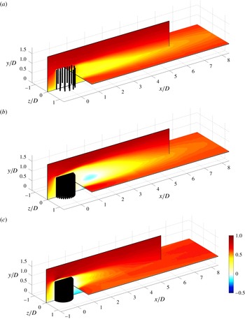
Figure 11. View of
 $U/U_{\infty }$
along the plane
$U/U_{\infty }$
along the plane
 $x$
–
$x$
–
 $y$
for
$y$
for
 $z=0$
and the plane
$z=0$
and the plane
 $x$
–
$x$
–
 $z$
for
$z$
for
 $y=D/2$
: (a)
$y=D/2$
: (a)
 $C_{20}$
, (b)
$C_{20}$
, (b)
 $C_{95}$
and (c)
$C_{95}$
and (c)
 $C_{S}$
. The cylinders are represented in their actual configuration.
$C_{S}$
. The cylinders are represented in their actual configuration.

Figure 12. View of
 $V/U_{\infty }$
in the vertical plane: (a)
$V/U_{\infty }$
in the vertical plane: (a)
 $C_{20}$
, (b)
$C_{20}$
, (b)
 $C_{39}$
(c)
$C_{39}$
(c)
 $C_{64}$
, (d)
$C_{64}$
, (d)
 $C_{95}$
and (e)
$C_{95}$
and (e)
 $C_{S}$
. The vector field only indicates the flow direction, but not its intensity (the length of the vectors is not proportional to their intensity). Only one vector every 35 vectors is represented. For the printed version, the solid black line is the contour where
$C_{S}$
. The vector field only indicates the flow direction, but not its intensity (the length of the vectors is not proportional to their intensity). Only one vector every 35 vectors is represented. For the printed version, the solid black line is the contour where
 $V/U_{\infty }=0.01$
and the solid grey line is the contour where
$V/U_{\infty }=0.01$
and the solid grey line is the contour where
 $V/U_{\infty }=-0.01$
. The cylinders are not drawn in their actual configuration, for the exact distribution of the cylinders at this plane, refer to figure 3.
$V/U_{\infty }=-0.01$
. The cylinders are not drawn in their actual configuration, for the exact distribution of the cylinders at this plane, refer to figure 3.
More insights on the wake of the patches are revealed by figure 12, which shows the non-dimensional vertical velocity component
 $V/U_{\infty }$
measured in the
$V/U_{\infty }$
measured in the
 $x$
–
$x$
–
 $y$
plane at
$y$
plane at
 $z=0$
. As for figures 9 and 10, unit velocity vectors are also shown to indicate the flow direction. As surmised from figure 10, figure 12 confirms that, for the solid case, the flow separates at the leading edge of the cylinder, reattaches along the top and convects downwards immediately downstream of the model. In
$z=0$
. As for figures 9 and 10, unit velocity vectors are also shown to indicate the flow direction. As surmised from figure 10, figure 12 confirms that, for the solid case, the flow separates at the leading edge of the cylinder, reattaches along the top and convects downwards immediately downstream of the model. In
 $C_{S}$
the vertical velocity shows the largest spatial variations in the flow field among all of the investigated cases. Furthermore,
$C_{S}$
the vertical velocity shows the largest spatial variations in the flow field among all of the investigated cases. Furthermore,
 $V/U_{\infty }$
has a localised positive peak in proximity of the leading-edge top, but becomes negative immediately downwind and remains so for almost the entire field of view. Figures 10 and 12 show that for the solid case the longitudinal extension of the recirculating region is not uniform along
$V/U_{\infty }$
has a localised positive peak in proximity of the leading-edge top, but becomes negative immediately downwind and remains so for almost the entire field of view. Figures 10 and 12 show that for the solid case the longitudinal extension of the recirculating region is not uniform along
 $y$
because it increases towards the wall. We interpret this as an effect of the shear layer at the free end, which contributes to strain the recirculation bubble by entraining momentum from the flow above the cylinder. The bubble enlarges towards the wall where free-end (i.e. top shear layer) effects are less intense.
$y$
because it increases towards the wall. We interpret this as an effect of the shear layer at the free end, which contributes to strain the recirculation bubble by entraining momentum from the flow above the cylinder. The bubble enlarges towards the wall where free-end (i.e. top shear layer) effects are less intense.
Compared with the solid case the porous patches behave very differently. The peaks of
 $V/U_{\infty }$
at the leading edge are lower in magnitude, presumably because of the permeability of the patches which allows for some fluid to go through their porous matrix rather then being all diverted upwards. For the same reason, the deceleration of the flow at the leading edge of the porous patches is less intense than for the solid case (see figure 10). Consistently with this hypothesis,
$V/U_{\infty }$
at the leading edge are lower in magnitude, presumably because of the permeability of the patches which allows for some fluid to go through their porous matrix rather then being all diverted upwards. For the same reason, the deceleration of the flow at the leading edge of the porous patches is less intense than for the solid case (see figure 10). Consistently with this hypothesis,
 $V/U_{\infty }$
at the top of the leading edge increases in magnitude with increasing
$V/U_{\infty }$
at the top of the leading edge increases in magnitude with increasing
 ${\it\phi}$
(figure 12) and also the mean longitudinal velocity
${\it\phi}$
(figure 12) and also the mean longitudinal velocity
 $U/U_{\infty }$
in front of the patch decreases with increasing
$U/U_{\infty }$
in front of the patch decreases with increasing
 ${\it\phi}$
(figure 10). At the free-end of the porous patches, the flow does not separate and the mean vertical velocity
${\it\phi}$
(figure 10). At the free-end of the porous patches, the flow does not separate and the mean vertical velocity
 $V$
remains positive, indicating that the flow bleeds upward from the interior of the patch (figure 12). At a heuristic level, this phenomenon can intuitively be ascribed to the pressure gradient generated by the difference in velocity between the faster flow that is immediately over the patch (that will result in lower pressure) and the slower flow within the patch (i.e. at higher pressure).
$V$
remains positive, indicating that the flow bleeds upward from the interior of the patch (figure 12). At a heuristic level, this phenomenon can intuitively be ascribed to the pressure gradient generated by the difference in velocity between the faster flow that is immediately over the patch (that will result in lower pressure) and the slower flow within the patch (i.e. at higher pressure).
At the trailing edge of the porous patches both
 $U$
and
$U$
and
 $V$
are also positive. We define
$V$
are also positive. We define
 $U_{bTE}$
and
$U_{bTE}$
and
 $V_{bTE}$
as the values of the mean longitudinal and vertical velocity components averaged over
$V_{bTE}$
as the values of the mean longitudinal and vertical velocity components averaged over
 $0<y/D<1$
at the trailing edge, which are reported in table 2. As observed from figure 9,
$0<y/D<1$
at the trailing edge, which are reported in table 2. As observed from figure 9,
 $U_{bTE}$
decreases with increasing density whereas, analogously to the vertical bleeding,
$U_{bTE}$
decreases with increasing density whereas, analogously to the vertical bleeding,
 $V_{bTE}$
increases. Therefore, with respect to the solid case, both the vertical and trailing edge bleeding are responsible for shifting upwards and further downwind the region of negative vertical velocity
$V_{bTE}$
increases. Therefore, with respect to the solid case, both the vertical and trailing edge bleeding are responsible for shifting upwards and further downwind the region of negative vertical velocity
 $V/U_{\infty }$
and, as already discussed, the recirculation bubble that forms in
$V/U_{\infty }$
and, as already discussed, the recirculation bubble that forms in
 $C_{64}$
and
$C_{64}$
and
 $C_{95}$
.
$C_{95}$
.
As it will be further discussed from the vorticity plots, the vertical and trailing edge bleeding contribute to weaken the free-end effects on the wake development. Consistently with this, the longitudinal extension of the recirculation bubble observed for
 $C_{64}$
and
$C_{64}$
and
 $C_{95}$
is independent of
$C_{95}$
is independent of
 $y$
, and the region is much less strained than in
$y$
, and the region is much less strained than in
 $C_{S}$
(figures 10 and 11).
$C_{S}$
(figures 10 and 11).
The contour plots of the mean vorticity along the spanwise (
 ${\it\omega}_{z}D/U_{\infty }$
) and wall-normal (
${\it\omega}_{z}D/U_{\infty }$
) and wall-normal (
 ${\it\omega}_{y}D/U_{\infty }$
) directions are given in figure 13. The chosen colour scale allows contours to saturate in some regions (i.e. at the top part of both
${\it\omega}_{y}D/U_{\infty }$
) directions are given in figure 13. The chosen colour scale allows contours to saturate in some regions (i.e. at the top part of both
 $C_{S}$
and
$C_{S}$
and
 $C_{95}$
) in order to ensure that variations of vorticity at lower levels are visible. Furthermore, for the printed version, we report the contours of
$C_{95}$
) in order to ensure that variations of vorticity at lower levels are visible. Furthermore, for the printed version, we report the contours of
 ${\it\omega}_{z}D/U_{\infty }=\pm 0.3$
and
${\it\omega}_{z}D/U_{\infty }=\pm 0.3$
and
 ${\it\omega}_{y}D/U_{\infty }=\pm 0.3$
to distinguish between positive and negative vorticity regions. The value of 0.3 was chosen to be as a reasonable threshold limit for vorticity to identify the boundaries of shear layers, which influence strongly wake entrainment and development. Figure 13 shows that
${\it\omega}_{y}D/U_{\infty }=\pm 0.3$
to distinguish between positive and negative vorticity regions. The value of 0.3 was chosen to be as a reasonable threshold limit for vorticity to identify the boundaries of shear layers, which influence strongly wake entrainment and development. Figure 13 shows that
 ${\it\omega}_{z}D/U_{\infty }$
over the top of the patches increases in intensity with increasing
${\it\omega}_{z}D/U_{\infty }$
over the top of the patches increases in intensity with increasing
 ${\it\phi}$
, especially in the top leading and trailing edges. In particular, the minimum
${\it\phi}$
, especially in the top leading and trailing edges. In particular, the minimum
 ${\it\omega}_{z}D/U_{\infty }$
(i.e. the maximum in absolute value) at
${\it\omega}_{z}D/U_{\infty }$
(i.e. the maximum in absolute value) at
 $x/D=0.75$
at the top of the trailing edge, which presumably has the strongest influence on the wake development downstream of the patch, increases in magnitude and elevation from the bed (i.e.
$x/D=0.75$
at the top of the trailing edge, which presumably has the strongest influence on the wake development downstream of the patch, increases in magnitude and elevation from the bed (i.e.
 $y/D$
) with increasing density (see table 2). This indicates that the higher is the density of the patch, the more intense is the shear layer and the more this is shifted upwards. This upward shift is due to the vertical bleeding, which, as observed in figure 12, also increases with increasing
$y/D$
) with increasing density (see table 2). This indicates that the higher is the density of the patch, the more intense is the shear layer and the more this is shifted upwards. This upward shift is due to the vertical bleeding, which, as observed in figure 12, also increases with increasing
 ${\it\phi}$
. The solid case is characterised by the strongest shear layers over both the top of the leading and trailing edge, although for the latter, due to the absence of vertical bleeding, the upwards shift cannot occur.
${\it\phi}$
. The solid case is characterised by the strongest shear layers over both the top of the leading and trailing edge, although for the latter, due to the absence of vertical bleeding, the upwards shift cannot occur.
The contour plots of the mean vorticity measured along the horizontal plane show that for the
 $C_{20}$
model, the wakes shed by individual cylinders are evident and detectable (see figure 13
b). However, two larger shear layers develop at the flanks of the patch, confirming also the presence of group behaviour.
$C_{20}$
model, the wakes shed by individual cylinders are evident and detectable (see figure 13
b). However, two larger shear layers develop at the flanks of the patch, confirming also the presence of group behaviour.
At
 $x/D=0.52$
, which corresponds to the most upwind location for our fields of view, these patch-scale shear layers retain the same width regardless of patch density (figure 13
b,d,f,h,j). This is consistent with what was observed from figure 9 and the fact that the width of the wake is weakly influenced by
$x/D=0.52$
, which corresponds to the most upwind location for our fields of view, these patch-scale shear layers retain the same width regardless of patch density (figure 13
b,d,f,h,j). This is consistent with what was observed from figure 9 and the fact that the width of the wake is weakly influenced by
 ${\it\phi}$
because, as already discussed, lateral bleeding fixes the separation point along the flanks of the patches, presumably at their most external cylinder. Further downwind, for all of the patch densities, the inner contour of the lateral shear layers show essentially two regions: one where they converge towards the centre of the wake and another where they either diverge or grow uniformly. The first region shrinks in length with increasing
${\it\phi}$
because, as already discussed, lateral bleeding fixes the separation point along the flanks of the patches, presumably at their most external cylinder. Further downwind, for all of the patch densities, the inner contour of the lateral shear layers show essentially two regions: one where they converge towards the centre of the wake and another where they either diverge or grow uniformly. The first region shrinks in length with increasing
 ${\it\phi}$
. This is consistent with the fact that, with increasing density, the trailing edge bleeding diminishes and the intensity of both the lateral and top shear layer increases, hence leading to stronger wake entrainment. Ultimately, for the solid case, the first region disappears and the two shear layers collapse and then disappear at a very short distance from the cylinder.
${\it\phi}$
. This is consistent with the fact that, with increasing density, the trailing edge bleeding diminishes and the intensity of both the lateral and top shear layer increases, hence leading to stronger wake entrainment. Ultimately, for the solid case, the first region disappears and the two shear layers collapse and then disappear at a very short distance from the cylinder.

Figure 13. Mean vorticity contours along the two PIV planes:
 ${\it\omega}_{z}D/U_{\infty }$
(a,c,e,g,i) and
${\it\omega}_{z}D/U_{\infty }$
(a,c,e,g,i) and
 ${\it\omega}_{y}D/U_{\infty }$
(b,d,f,h,j). Panels in rows (a,b), (c,d), (e,f), (g,h) and (i,j) are for the models
${\it\omega}_{y}D/U_{\infty }$
(b,d,f,h,j). Panels in rows (a,b), (c,d), (e,f), (g,h) and (i,j) are for the models
 $C_{20}$
,
$C_{20}$
,
 $C_{39}$
 $C_{64}$
,
$C_{64}$
,
 $C_{95}$
and
$C_{95}$
and
 $C_{S}$
, respectively. For the printed version, the solid black line is the contour where
$C_{S}$
, respectively. For the printed version, the solid black line is the contour where
 ${\it\omega}D/U_{\infty }=0.3$
and the solid grey line is the contour where
${\it\omega}D/U_{\infty }=0.3$
and the solid grey line is the contour where
 ${\it\omega}_{z}D/U_{\infty }=-0.3$
. The plot of
${\it\omega}_{z}D/U_{\infty }=-0.3$
. The plot of
 ${\it\omega}_{z}$
is saturated at the top for some cases, but a different colour scale would not allow the contours to be seen in the other cases. For the plots in the vertical plane the cylinders are not drawn in their actual configuration, which is represented only for the horizontal plane.
${\it\omega}_{z}$
is saturated at the top for some cases, but a different colour scale would not allow the contours to be seen in the other cases. For the plots in the vertical plane the cylinders are not drawn in their actual configuration, which is represented only for the horizontal plane.
Interestingly, the shear layers developing at the flanks and over the top of the patches (figures 13
b,d,f,h,j and 13
a,c,e,g,i, respectively) show a different behaviour with respect to
 ${\it\phi}$
. While they both increase in intensity with increasing density, the top shear layers show much larger variations with respect to
${\it\phi}$
. While they both increase in intensity with increasing density, the top shear layers show much larger variations with respect to
 ${\it\phi}$
, particularly between
${\it\phi}$
, particularly between
 $C_{95}$
and
$C_{95}$
and
 $C_{S}$
. In particular, the maximum
$C_{S}$
. In particular, the maximum
 ${\it\omega}_{y}D/U_{\infty }$
at
${\it\omega}_{y}D/U_{\infty }$
at
 $x/D=0.75$
at the flanks of the models (see table 2) increases by about 23 % from
$x/D=0.75$
at the flanks of the models (see table 2) increases by about 23 % from
 $C_{95}$
to
$C_{95}$
to
 $C_{S}$
while
$C_{S}$
while
 ${\it\omega}_{z}D/U_{\infty }$
almost doubles at the same streamwise location for the same models. In other words the difference in the intensity of vorticity between
${\it\omega}_{z}D/U_{\infty }$
almost doubles at the same streamwise location for the same models. In other words the difference in the intensity of vorticity between
 $C_{95}$
and
$C_{95}$
and
 $C_{S}$
is larger for the shear layers at the top than at the flanks. This can be explained by the following argument: due to their packing and geometry, vertical cylinders within each patch form a porous medium characterised by an anisotropic permeability. In particular, the permeability along the vertical direction is much higher than the permeability along all directions lying on the
$C_{S}$
is larger for the shear layers at the top than at the flanks. This can be explained by the following argument: due to their packing and geometry, vertical cylinders within each patch form a porous medium characterised by an anisotropic permeability. In particular, the permeability along the vertical direction is much higher than the permeability along all directions lying on the
 $x$
–
$x$
–
 $z$
plane. As shown by Manes, Poggi & Ridolfi (Reference Manes, Poggi and Ridolfi2011a
), Manes et al. (Reference Manes, Pokrajac, Nikora, Ridolfi and Poggi2011b
), Manes, Ridolfi & Katul (Reference Manes, Ridolfi and Katul2012), enhanced permeability favours momentum transport at the interface between a turbulent flow and a permeable canopy, which weakens the velocity gradient at the canopy top and ultimately the intensity of the associated shear layer. When switching from
$z$
plane. As shown by Manes, Poggi & Ridolfi (Reference Manes, Poggi and Ridolfi2011a
), Manes et al. (Reference Manes, Pokrajac, Nikora, Ridolfi and Poggi2011b
), Manes, Ridolfi & Katul (Reference Manes, Ridolfi and Katul2012), enhanced permeability favours momentum transport at the interface between a turbulent flow and a permeable canopy, which weakens the velocity gradient at the canopy top and ultimately the intensity of the associated shear layer. When switching from
 $C_{S}$
to
$C_{S}$
to
 $C_{95}$
, the permeability for the vertical component over the patch top increases much more than the permeability associated with lateral flow movements at the flanks. This explains why the differences in shear layer intensity between
$C_{95}$
, the permeability for the vertical component over the patch top increases much more than the permeability associated with lateral flow movements at the flanks. This explains why the differences in shear layer intensity between
 $C_{95}$
and
$C_{95}$
and
 $C_{S}$
are larger at the top than at the flanks of the patches.
$C_{S}$
are larger at the top than at the flanks of the patches.
4 Discussion
4.1 Bleeding effects in 3D patches
From a momentum balance point of view, the drag coefficient of an obstacle is mainly influenced by the spread of its wake and the intensity of the velocity deficit in the wake itself. For porous patches, there are three main flow phenomena which affect the wake compared with a solid body: (i) the lateral bleeding, (ii) the vertical bleeding and (iii) the trailing edge bleeding.
The lateral bleeding prevents the reattachment of the flow along the sides of the porous patches hence contributing to widening their wake. The effect of the vertical bleeding (always upwards for porous patches, as observed in figure 10) is twofold: (i) it pushes upwards the shear layer forming at the patch-top hence enlarging the vertical size of the wake; and (ii) it weakens wake entrainment. This last effect is due to the positive vertical velocity generated immediately downwind of the trailing edge (i.e.
 $V_{bTE}$
) which prevents the lower boundary of top shear layer to develop downwards and ultimately weakens the entrainment of fluid in the wake.
$V_{bTE}$
) which prevents the lower boundary of top shear layer to develop downwards and ultimately weakens the entrainment of fluid in the wake.
We conclude that both lateral and vertical edge bleeding contribute to either enlarge the size of the wake along
 $z$
and
$z$
and
 $y$
or to prevent wake entrainment. Both effects contribute to increase flow resistance, meaning that an increase in bleeding contributes to an increase of the patch drag coefficient
$y$
or to prevent wake entrainment. Both effects contribute to increase flow resistance, meaning that an increase in bleeding contributes to an increase of the patch drag coefficient
 $C_{D}$
.
$C_{D}$
.
Conversely, the trailing edge bleeding has the opposite effect. In fact
 $U_{bTE}$
contributes to diminish the velocity deficit in the wake and hence to lower
$U_{bTE}$
contributes to diminish the velocity deficit in the wake and hence to lower
 $C_{D}$
. Furthermore the trailing edge bleeding causes the recirculation region (if any) to move downstream, and decreases the intensity of the shear layers forming at the sides, which also contribute to lower
$C_{D}$
. Furthermore the trailing edge bleeding causes the recirculation region (if any) to move downstream, and decreases the intensity of the shear layers forming at the sides, which also contribute to lower
 $C_{D}$
.
$C_{D}$
.
4.2 Interlinks between bleeding, patch density and
 $C_{D}$

Bleeding effects help to explain the behaviour of
 $C_{D}$
versus
$C_{D}$
versus
 ${\it\phi}$
as depicted by figure 7. The relation between the patch density
${\it\phi}$
as depicted by figure 7. The relation between the patch density
 ${\it\phi}$
and the intensity of the trailing edge bleeding
${\it\phi}$
and the intensity of the trailing edge bleeding
 $U_{bTE}$
can be observed in table 2. An increase in
$U_{bTE}$
can be observed in table 2. An increase in
 ${\it\phi}$
corresponds to a reduction of the bleeding at the trailing edge, which in turn corresponds to an increase in the velocity deficit and hence in
${\it\phi}$
corresponds to a reduction of the bleeding at the trailing edge, which in turn corresponds to an increase in the velocity deficit and hence in
 $C_{D}$
, consistently with figure 7.
$C_{D}$
, consistently with figure 7.
An increase in
 ${\it\phi}$
also results in an increase of bleeding along the vertical direction (figure 10, table 2) which, as discussed, contributes to increase
${\it\phi}$
also results in an increase of bleeding along the vertical direction (figure 10, table 2) which, as discussed, contributes to increase
 $C_{D}$
and this is also consistent with figure 7.
$C_{D}$
and this is also consistent with figure 7.
The lateral extension of the wake does not seem to change much with
 ${\it\phi}$
(figure 9) and therefore we conclude that the observed increase of
${\it\phi}$
(figure 9) and therefore we conclude that the observed increase of
 $C_{D}$
with increasing
$C_{D}$
with increasing
 ${\it\phi}$
must be predominantly due to the increasing of vertical bleeding and the decrease of trailing edge bleeding with
${\it\phi}$
must be predominantly due to the increasing of vertical bleeding and the decrease of trailing edge bleeding with
 ${\it\phi}$
. This last comment should not be misinterpreted. While lateral bleeding seems to have the only effect of fixing the lateral separation point around the patches and hence to have a minor role in explaining the dependence of
${\it\phi}$
. This last comment should not be misinterpreted. While lateral bleeding seems to have the only effect of fixing the lateral separation point around the patches and hence to have a minor role in explaining the dependence of
 $C_{D}$
on
$C_{D}$
on
 ${\it\phi}$
, this does not mean that it does not have a role in dictating the absolute values of
${\it\phi}$
, this does not mean that it does not have a role in dictating the absolute values of
 $C_{D}$
for porous patches. This will be discussed more in detail in § 4.4.
$C_{D}$
for porous patches. This will be discussed more in detail in § 4.4.
4.3 2D versus 3D patches
Figure 8 shows that the
 $C_{Dbulk}$
reported in the present paper for 3D patches are lower than those reported in the literature for 2D patches, and the difference increases for increasing densities. Presumably, this difference must be associated with top shear layer effects (i.e. the bleeding along
$C_{Dbulk}$
reported in the present paper for 3D patches are lower than those reported in the literature for 2D patches, and the difference increases for increasing densities. Presumably, this difference must be associated with top shear layer effects (i.e. the bleeding along
 $y$
) and, perhaps, incoming turbulence, which was absent in the 2D cases investigated in the literature. In fact, incoming turbulence can delay separation around bluff bodies and hence contribute to explain the observed discrepancies in
$y$
) and, perhaps, incoming turbulence, which was absent in the 2D cases investigated in the literature. In fact, incoming turbulence can delay separation around bluff bodies and hence contribute to explain the observed discrepancies in
 $C_{D}$
. However, in the case of a porous patch, this is unlikely to happen because the separation point is fixed by lateral bleeding. Even though the separation point around an individual cylinder of the patches may vary its location, such variations occur at very small scales (i.e. at the scale of
$C_{D}$
. However, in the case of a porous patch, this is unlikely to happen because the separation point is fixed by lateral bleeding. Even though the separation point around an individual cylinder of the patches may vary its location, such variations occur at very small scales (i.e. at the scale of
 $d$
) and hence they cannot affect the overall lateral dimension of the wake at the patch scale and ultimately its drag coefficient.
$d$
) and hence they cannot affect the overall lateral dimension of the wake at the patch scale and ultimately its drag coefficient.
The top shear layer effects are dramatically evident in the case of a solid cylinder, where the drop in
 $C_{Dbulk}$
is about 67 % compared with Nicolle & Eames (Reference Nicolle and Eames2011) and 50 % compared with Chang & Constantinescu (Reference Chang and Constantinescu2015) (figure 8). It has to be noted that, for the solid case, the incoming turbulence concurs to enlarge this difference by promoting entrainment on the top of the cylinder.
$C_{Dbulk}$
is about 67 % compared with Nicolle & Eames (Reference Nicolle and Eames2011) and 50 % compared with Chang & Constantinescu (Reference Chang and Constantinescu2015) (figure 8). It has to be noted that, for the solid case, the incoming turbulence concurs to enlarge this difference by promoting entrainment on the top of the cylinder.
The discrepancy in
 $C_{Dbulk}$
between 2D and 3D porous patches is much less intense compared with their solid counterpart and decreases with decreasing
$C_{Dbulk}$
between 2D and 3D porous patches is much less intense compared with their solid counterpart and decreases with decreasing
 ${\it\phi}$
(up to 34 % for the densest patch, less than 15 % for the other cases). This is due to the fact that free-end (i.e. 3D) effects in the form of the top shear layer intensity (i.e.
${\it\phi}$
(up to 34 % for the densest patch, less than 15 % for the other cases). This is due to the fact that free-end (i.e. 3D) effects in the form of the top shear layer intensity (i.e.
 ${\it\omega}_{zMAX}D/U_{\infty }$
) and the vertical bleeding (i.e.
${\it\omega}_{zMAX}D/U_{\infty }$
) and the vertical bleeding (i.e.
 $V_{bTE}$
) decrease with decreasing
$V_{bTE}$
) decrease with decreasing
 ${\it\phi}$
(see table 2).
${\it\phi}$
(see table 2).
4.4 Solid versus dense patches
So far we have predominantly discussed the drag coefficient for porous patches and their dependence on the density
 ${\it\phi}$
. However, the most striking and counterintuitive result of the present paper emerges from the comparison between the drag coefficients of the porous and the solid cases. In particular, figures 7 and 8 show that the drag coefficient of a solid cylinder is much lower than the
${\it\phi}$
. However, the most striking and counterintuitive result of the present paper emerges from the comparison between the drag coefficients of the porous and the solid cases. In particular, figures 7 and 8 show that the drag coefficient of a solid cylinder is much lower than the
 $C_{D}$
of a patch having the largest investigated density. Now that the mechanisms linking drag with bleeding have been clarified, this result can be easily explained. For the solid cylinder, the intense shear layers forming around its surface and the absence of lateral and vertical bleeding promote strong wake entrainment, which contributes to narrow significantly the wake size along
$C_{D}$
of a patch having the largest investigated density. Now that the mechanisms linking drag with bleeding have been clarified, this result can be easily explained. For the solid cylinder, the intense shear layers forming around its surface and the absence of lateral and vertical bleeding promote strong wake entrainment, which contributes to narrow significantly the wake size along
 $y$
and
$y$
and
 $z$
and ultimately to lower the drag coefficient
$z$
and ultimately to lower the drag coefficient
 $C_{D}$
. Clearly, the zero bleeding at the trailing edge of the solid surface is not able to counteract all of these effects and hence the
$C_{D}$
. Clearly, the zero bleeding at the trailing edge of the solid surface is not able to counteract all of these effects and hence the
 $C_{D}$
of the solid cylinder results much lower than the
$C_{D}$
of the solid cylinder results much lower than the
 $C_{D}$
of
$C_{D}$
of
 $C_{95}$
where vertical and lateral bleeding effects are instead very strong. The end result is that the
$C_{95}$
where vertical and lateral bleeding effects are instead very strong. The end result is that the
 $C_{D}$
of the solid cylinder is actually comparable to the case
$C_{D}$
of the solid cylinder is actually comparable to the case
 $C_{20}$
, which was an unexpected result.
$C_{20}$
, which was an unexpected result.
In order to see which of the bleeding processes is most responsible for the differences in drag between the solid and the dense patch, one more drag measurement was carried out. This was performed by gluing a circular wooden plate on top of the
 $C_{95}$
model. This experiment was designed to weaken the effects of the vertical bleeding at the patch-top (model named
$C_{95}$
model. This experiment was designed to weaken the effects of the vertical bleeding at the patch-top (model named
 $C_{95T}$
) and to increase the intensity of the top shear layer. This experiment showed that the drag coefficient of the patch with a lid on top is close to the drag coefficient of the
$C_{95T}$
) and to increase the intensity of the top shear layer. This experiment showed that the drag coefficient of the patch with a lid on top is close to the drag coefficient of the
 $C_{95}$
model (namely
$C_{95}$
model (namely
 $C_{D}=$
0.371 for
$C_{D}=$
0.371 for
 $C_{95T}$
, versus
$C_{95T}$
, versus
 $C_{D}=0.374$
for
$C_{D}=0.374$
for
 $C_{95}$
). Hence, this last experiment indicates that while the dependence of
$C_{95}$
). Hence, this last experiment indicates that while the dependence of
 $C_{D}$
on
$C_{D}$
on
 ${\it\phi}$
is strongly linked to top shear layer effects, the differences between the
${\it\phi}$
is strongly linked to top shear layer effects, the differences between the
 $C_{95}$
and
$C_{95}$
and
 $C_{S}$
seems to be more dictated by lateral bleeding effects. More in general, this experiment also suggests that, while differences in
$C_{S}$
seems to be more dictated by lateral bleeding effects. More in general, this experiment also suggests that, while differences in
 $C_{D}$
for different
$C_{D}$
for different
 ${\it\phi}$
are dictated mainly by vertical and trailing edge bleeding, lateral bleeding still plays an important role in the game of drag generation, although this is weakly dependent on
${\it\phi}$
are dictated mainly by vertical and trailing edge bleeding, lateral bleeding still plays an important role in the game of drag generation, although this is weakly dependent on
 ${\it\phi}$
.
${\it\phi}$
.
As a side note we further discuss the results by Chang & Constantinescu (Reference Chang and Constantinescu2015) who also observed a drop in
 $C_{D}$
between a dense (where dense means with a density similar to our
$C_{D}$
between a dense (where dense means with a density similar to our
 $C_{95}$
case) and a solid 2D patch. Chang & Constantinescu (Reference Chang and Constantinescu2015) observed that the pressure distribution around a solid and a dense 2D patch is almost the same and hence they argued that this must lead to the build up of comparable pressure drag. However, with respect to the solid case, they also argued that a porous patch experiences some extra drag due to the resistance offered to the flow by internal cylinders and this explains the drop in drag coefficient observed for solid patches. We point out that, if the explanation given by Chang & Constantinescu (Reference Chang and Constantinescu2015) holds, the same drop in
$C_{95}$
case) and a solid 2D patch. Chang & Constantinescu (Reference Chang and Constantinescu2015) observed that the pressure distribution around a solid and a dense 2D patch is almost the same and hence they argued that this must lead to the build up of comparable pressure drag. However, with respect to the solid case, they also argued that a porous patch experiences some extra drag due to the resistance offered to the flow by internal cylinders and this explains the drop in drag coefficient observed for solid patches. We point out that, if the explanation given by Chang & Constantinescu (Reference Chang and Constantinescu2015) holds, the same drop in
 $C_{D}$
between the solid and the dense case should have also been detected by Nicolle & Eames (Reference Nicolle and Eames2011), but this is not the case. Therefore, we argue that this mechanism cannot explain the differences in drag between the solid and the dense porous patch. As already discussed, such differences must be rather associated with the more intense shear layers (see figure 13 and table 2) developing around solid patches, which promote wake entrainment and hence drag reduction. Such an entrainment is prevented in porous dense patches because of bleeding along directions perpendicular to the mean flow.
$C_{D}$
between the solid and the dense case should have also been detected by Nicolle & Eames (Reference Nicolle and Eames2011), but this is not the case. Therefore, we argue that this mechanism cannot explain the differences in drag between the solid and the dense porous patch. As already discussed, such differences must be rather associated with the more intense shear layers (see figure 13 and table 2) developing around solid patches, which promote wake entrainment and hence drag reduction. Such an entrainment is prevented in porous dense patches because of bleeding along directions perpendicular to the mean flow.
The last question that remains to be answered is: why was the drop in
 $C_{D}$
for the solid cylinder not also reported by Nicolle & Eames (Reference Nicolle and Eames2011)? We argue that the low Reynolds number of the simulations that these authors carried out allowed solid cylinders to be associated with higher values of
$C_{D}$
for the solid cylinder not also reported by Nicolle & Eames (Reference Nicolle and Eames2011)? We argue that the low Reynolds number of the simulations that these authors carried out allowed solid cylinders to be associated with higher values of
 $C_{D}$
due to the earlier separation of the flow along the sides of the cylinders, which laterally enlarges the wake and increases the drag coefficient to a value which is comparable to that of the densest patch.
$C_{D}$
due to the earlier separation of the flow along the sides of the cylinders, which laterally enlarges the wake and increases the drag coefficient to a value which is comparable to that of the densest patch.
5 Conclusions
This paper presents an experimental study devoted to investigate the interlinks between drag coefficient and wake properties of cylindrical canopy patches by varying extensively the canopy density
 ${\it\phi}$
. The novelty of the work lies in the fact that, to the best of the authors’ knowledge, this is the first study addressing the case of patches that are fully submerged within a turbulent boundary layer. Our results show that, within the range of
${\it\phi}$
. The novelty of the work lies in the fact that, to the best of the authors’ knowledge, this is the first study addressing the case of patches that are fully submerged within a turbulent boundary layer. Our results show that, within the range of
 ${\it\phi}$
investigated herein, the drag coefficient of porous patches increases with increasing
${\it\phi}$
investigated herein, the drag coefficient of porous patches increases with increasing
 ${\it\phi}$
. However, the coefficient of a solid case with the same external dimensions is almost half of the maximum value obtained for porous patches.
${\it\phi}$
. However, the coefficient of a solid case with the same external dimensions is almost half of the maximum value obtained for porous patches.
It was pointed out that the increase of the drag coefficient
 $C_{D}$
with increasing
$C_{D}$
with increasing
 ${\it\phi}$
is associated with an increase of vertical bleeding as well as a decrease in trailing edge bleeding. In particular, the increase in vertical bleeding promotes wake enlargement as well as working against wake entrainment. A decrease in trailing edge bleeding, instead, contributes towards developing more intense velocity deficits. Wake enlargement, strong velocity deficits and weaker wake entrainment all contribute towards the development of higher
${\it\phi}$
is associated with an increase of vertical bleeding as well as a decrease in trailing edge bleeding. In particular, the increase in vertical bleeding promotes wake enlargement as well as working against wake entrainment. A decrease in trailing edge bleeding, instead, contributes towards developing more intense velocity deficits. Wake enlargement, strong velocity deficits and weaker wake entrainment all contribute towards the development of higher
 $C_{D}$
.
$C_{D}$
.
Particular attention was paid to explain the counterintuitive drop in
 $C_{D}$
observed between the densest porous case and the solid case. Our velocity measurements helped explaining that the drop in
$C_{D}$
observed between the densest porous case and the solid case. Our velocity measurements helped explaining that the drop in
 $C_{D}$
is associated with the development of strong shear layers around the solid patch, which contribute to wake entrainment and hence to reduce
$C_{D}$
is associated with the development of strong shear layers around the solid patch, which contribute to wake entrainment and hence to reduce
 $C_{D}$
. The effect of these shear layers is weakened in the case of the densest porous patch, because of significant lateral and vertical bleeding. In particular, it was argued that lateral bleeding could play a more important role than vertical bleeding in explaining the differences between the
$C_{D}$
. The effect of these shear layers is weakened in the case of the densest porous patch, because of significant lateral and vertical bleeding. In particular, it was argued that lateral bleeding could play a more important role than vertical bleeding in explaining the differences between the
 $C_{D}$
of the dense and the solid patch.
$C_{D}$
of the dense and the solid patch.
We point out that, due to experimental constraints, the
 $C_{D}$
versus
$C_{D}$
versus
 ${\it\phi}$
curves presented in figures 7 and 8 show a big gap of data for
${\it\phi}$
curves presented in figures 7 and 8 show a big gap of data for
 $0.24<{\it\phi}<1$
. This lack of data calls for more experiments to investigate whether for
$0.24<{\it\phi}<1$
. This lack of data calls for more experiments to investigate whether for
 $0.24<{\it\phi}<1$
the drag coefficient reaches a plateau and then abruptly decreases after a threshold value of density, or whether it shows a maximum and then smoothly decreases towards the solid case value.
$0.24<{\it\phi}<1$
the drag coefficient reaches a plateau and then abruptly decreases after a threshold value of density, or whether it shows a maximum and then smoothly decreases towards the solid case value.
As a final comment, our experimental results suggests that porous obstacles act as very efficient momentum sinks (i.e. more efficient than their solid counterpart), when immersed in a turbulent boundary layer. We suggest that this result could be exploited for engineering applications that require to maximise flow resistance while maintaining low roughness densities (i.e. number of roughness elements per unit surface). For example, fish passes at steep slopes are commonly built using roughness elements to minimise mean velocities (i.e. maximise flow resistance) while maintaining a healthy spacing between elements (usually in the form of rocks or artificial baffles) to allow for upstream fish migration (Armstrong et al. Reference Armstrong, Aprahamian, Fewings, Gough, Reader and Varallo2010). Our results suggest that replacing solid with porous roughness elements (e.g. vegetation-like surfaces) could lead to an enhanced flow resistance and ultimately an improved fish pass efficiency.
Acknowledgements
We gratefully acknowledge the financial support from the European Research Council (ERC grant agreement no. 277472), EPSRC Doctoral training grant and grant ref no. EP/I037717/1. We are also grateful to Dr C. Vanderwel for her comments on an early version of this manuscript. All data supporting this study are openly available from the University of Southampton repository http://dx.doi.org/10.5258/SOTON/393575.


