


1 Introduction
Marine propulsors and control surfaces are typically manufactured from metallic alloys due to their high stiffness and resistance to both corrosion fatigue and cavitation erosion. There has been extensive research conducted on the performance of metal propellers focusing on the relatively simple decoupled hydrodynamic and structural analysis (Young et al. Reference Young, Garg, Brandner, Pearce, Butler, Clarke and Phillips2018a). However, due to the high cost associated with machining the complex geometry of a propeller and poor acoustic damping properties of metallic alloys (Mouritz et al. Reference Mouritz, Gellert, Burchill and Challis2001), the use of alternative materials has recently been investigated (Young Reference Young2008). Composite materials offer high-strength-to-weight and stiffness-to-weight ratios that lead to significant weight reduction, allowing the construction of flexible hydrofoils that improve hydrodynamic performance and increase cavitation inception speeds through passive load-dependent shape adaptation (Young et al. Reference Young, Motley, Barber, Chae and Garg2016, Reference Young, Harwood, Montero, Ward and Ceccio2017). From extensive testing on a range of marine vessels, Ashkenazi et al. (Reference Ashkenazi, Golfman, Rezhkov and Sidorov1974) showed that the performance of several composite propellers was virtually equal to that of a metal counterpart in terms of speed, fuel consumption and engine workload, but significantly reduced engine and shaft vibrations.

Figure 1. Cloud cavitation about a finite span hydrofoil exhibiting multiple shedding events along the span due to the re-entrant jet instability and spanwise compatibility of the cavitation. The hydrofoil is vertically mounted at an incidence of  $6^{\circ }$ to the flow with chord-based Reynolds number
  $Re=0.8\times 10^{6}$ and
  $\unicode[STIX]{x1D70E}=0.7$.
However, these propellers did not exploit hydroelastic tailoring where the anisotropic characteristics of laminated fibre composites can be utilised to tailor blade deformations for improved performance. This flexibility introduces complex fluid–structure interaction (FSI) phenomena, particularly in cavitating conditions as shown in figure 1 and discussed by Smith et al. (Reference Smith, Venning, Pearce, Young and Brandner2020) (hereafter referred to as Part 1), that are not fully understood and need to be investigated. Developments made in the construction of composite structures has led to the hydroelastic tailoring of hydrofoils where geometric aspects are tailored to achieve a desired passive structural response based on the loading distribution to improve performance (Young Reference Young2007, Reference Young2008; Young et al. Reference Young, Motley, Barber, Chae and Garg2016, Reference Young, Harwood, Montero, Ward and Ceccio2017). The material-induced bend–twist coupling deflections affect flow separation, cavitation behaviour (Pearce et al. Reference Pearce, Brandner, Garg, Young, Phillips and Clarke2017; Smith et al. Reference Smith, Venning, Brandner, Pearce, Giosio and Young2018; Young et al. Reference Young, Garg, Brandner, Pearce, Butler, Clarke and Phillips2018b; Liao, Martins & Young Reference Liao, Martins and Young2019; Smith et al. Reference Smith, Venning, Giosio, Brandner, Pearce and Young2019b), inception boundaries, modal vibration characteristics (Akcabay & Young Reference Akcabay and Young2014; Akcabay et al. Reference Akcabay, Chae, Young, Ducoin and Astolfi2014; Akcabay & Young Reference Akcabay and Young2015) and hydroelastic instability boundaries (Young et al. Reference Young, Garg, Brandner, Pearce, Butler, Clarke and Phillips2018a; Harwood et al. Reference Harwood, Felli, Falchi, Garg, Ceccio and Young2019, Reference Harwood, Felli, Falchi, Garg, Ceccio and Young2020). This self-adaptive behaviour has been utilised in the development of composite propellers (Young Reference Young2008; Motley, Liu & Young Reference Motley, Liu and Young2009; Young et al. Reference Young, Motley, Barber, Chae and Garg2016) and active control surfaces (Turnock & Wright Reference Turnock and Wright2000; Young et al. Reference Young, Garg, Brandner, Pearce, Butler, Clarke and Phillips2018a) to improve energy efficiency as well as delaying and mitigating the adverse effects of cavitation. One of these effects is the unsteady loading and vibration induced by the shedding of cloud cavitation.
As discussed in Part 1, the presence of unsteady cloud cavitation about a hydrofoil has a significant effect on the structural response, even when the hydrofoil is relatively stiff. The unsteady two-phase flow is shown to cause frequency modulation (Akcabay & Young Reference Akcabay and Young2015), broaden the frequency content (Akcabay et al. Reference Akcabay, Chae, Young, Ducoin and Astolfi2014) and lock-in (Kato, Dan & Matsudaira Reference Kato, Dan and Matsudaira2006; Akcabay & Young Reference Akcabay and Young2015). Due to FSI, the structural response is seen to modify the cavity dynamics as well (Ausoni et al. Reference Ausoni, Farhat, Escaler, Egusquiza and Avellan2007; Ducoin, Astolfi & Sigrist Reference Ducoin, Astolfi and Sigrist2012; Wu et al. Reference Wu, Huang, Wang and Gao2015) with Akcabay et al. (Reference Akcabay, Chae, Young, Ducoin and Astolfi2014) showing greater hydrofoil compliance caused increased cavity length, resulting in a reduction of the shedding frequency.
Experiments using composite hydrofoils with varying anisotropic characteristics were conducted by Pearce et al. (Reference Pearce, Brandner, Garg, Young, Phillips and Clarke2017) and Young et al. (Reference Young, Garg, Brandner, Pearce, Butler, Clarke and Phillips2018b) to investigate the influence of hydroelastic tailoring on hydrofoil performance in cavitating conditions. The hydrofoil featured fibre orientation that resulted in bending-up and nose-up material-induced bend–twist coupling was observed to accelerate cavitation inception, increase cavity length and reduce shedding frequency compared to the relatively stiff reference due to the increased effective angle of attack. The opposite was observed for the hydrofoil with fibre orientations resulting in negative material-induced bend–twist coupling. However, global shedding dynamics was deemed dominant over any FSI effect in determining the resultant structural behaviour at low cavitation numbers (Pearce et al. Reference Pearce, Brandner, Garg, Young, Phillips and Clarke2017).
Smith et al. (Reference Smith, Venning, Brandner, Pearce, Giosio and Young2018) and Smith et al. (Reference Smith, Venning, Giosio, Brandner, Pearce and Young2019b) conducted experiments using a composite hydrofoil principally exhibiting tip bending deformations by utilising certain fibre orientations in the lay-up of the hydrofoil. It was shown that the hydrofoil’s compliance increased the magnitude of the force fluctuations for the low-frequency shockwave-driven shedding, compared to the relatively stiff hydrofoil. However, hydrofoil compliance was seen to dampen the fluctuating magnitude of the higher-frequency re-entrant jet-driven modes. Furthermore, the cavitation pattern over the flexible hydrofoil was also altered compared to the stiff hydrofoil with both streamwise and spanwise characteristics being affected. These alterations included cavity length, cavitation cloud width and spanwise shedding location with similar observations made by Pearce et al. (Reference Pearce, Brandner, Garg, Young, Phillips and Clarke2017) and Young et al. (Reference Young, Garg, Brandner, Pearce, Butler, Clarke and Phillips2018b). In spite of the advantages that the use of composite material may bring in regard to performance, composite materials tend to be more susceptible to cavitation erosion damage (Young et al. Reference Young, Motley, Barber, Chae and Garg2016), and hence the choice of surface coating must be carefully considered.
The influence of FSI on cloud cavitation about a hydrofoil is examined through experiments conducted on a composite hydrofoil with fibres orientated to consider principally bending deformations, i.e. without material bend–twist coupling. The results and discussions are complemented by those made in Part 1 on the relatively stiff reference hydrofoil. Experiments were conducted in the same manner outlined in Part 1 where forces acting on the hydrofoil were acquired simultaneously with tip deflections and cavitation behaviour measurements using high-speed photography. Differences observed in the results between hydrofoils are attributed to FSI effects.
2 Experimental overview
The experimental set-up and techniques utilised in the investigation were as previously described in Part 1 and are therefore only briefly summarised. Detailed descriptions are reserved for unique aspects of Part 2 of the experiment not previously described in Part 1.
2.1 Experimental facility
Testing was undertaken at the Australian Maritime College in the Cavitation Research Laboratory water tunnel with a detailed description of the facility given in Brandner, Lecoffre & Walker (Reference Brandner, Lecoffre and Walker2007). Measurements were repeated for the flexible hydrofoil in the same conditions as for the stiff hydrofoil where it was mounted at a fixed incidence,  $\unicode[STIX]{x1D6FC}$, of
  $6^{\circ }$ and tested at a chord-based Reynolds number,
  $Re=U_{\infty }\bar{c}/\unicode[STIX]{x1D708}$, equal to
  $0.8\times 10^{6}$, where
  $\bar{c}$ is the mean chord,
  $U_{\infty }$ is the free-stream velocity and
  $\unicode[STIX]{x1D708}$ is the kinematic viscosity of the water. The cavitation number,
  $\unicode[STIX]{x1D70E}=2(p_{\infty }-p_{v})/\unicode[STIX]{x1D70C}U_{\infty }^{2}$, where
  $p_{\infty }$ is the absolute static pressure at the level of the hydrofoil tip,
  $p_{v}$ is the vapour pressure and
  $\unicode[STIX]{x1D70C}$ is the water density, was incrementally varied from
  $1.2$ to
  $0.2$ to investigate various cavitation regimes. Dissolved oxygen levels were kept between
  $3$ and
  $4$ ppm for all measurements.
The flexible hydrofoil, described in § 2.2, was attached to a six-component force balance, with an estimated precision of  $0.1\,\%$, via a housing that clamped the hydrofoil in place using two profiled plates (figure 2), as for the stiff hydrofoil.

Figure 2. Hydrofoil model assembly showing an exploded view of the clamping housing arrangement allowing continuity of the hydrofoil.
2.2 Model hydrofoil
The flexible hydrofoil features an identical undeformed geometry to the stiff hydrofoil described in Part 1 with a symmetric (unswept) trapezoidal planform of  $300~\text{mm}$ span,
  $b$, a
  $60~\text{mm}$ tip chord and
  $120~\text{mm}$ root chord resulting in a mean chord,
  $\bar{c}$, of
  $90~\text{mm}$. The hydrofoils feature an extended base section for the reinforcing fibres in the flexible hydrofoil to run continuously, resulting in cantilevered structural boundary conditions by providing sufficient clamping length (Young et al. Reference Young, Garg, Brandner, Pearce, Butler, Clarke and Phillips2018a). The modified NACA0009 section profile features a thicker trailing edge for improved manufacturing of the flexible composite hydrofoil. Both hydrofoils are manufactured to a
  $\pm 0.1~\text{mm}$ surface tolerance and
  $0.8~\unicode[STIX]{x03BC}\text{m}$ surface finish. Despite the efforts made, small imperfections were still evident on the surface of the composite hydrofoil. Their influence on cavitation behaviour is discussed later in § 3.4.5.

Figure 3. Lay-up sequence of the flexible composite hydrofoil.
The composite hydrofoil model was manufactured as a carbon/glass-epoxy hybrid structure using a closed mould resin transfer moulding process. A two-part epoxy system (Kinetix R118/H103 manufactured by ATL Composites) was used for the matrix resin due to its low viscosity and long pot life properties. The structural component of the hydrofoil comprised of layers of T700 unidirectional carbon fibre (Carbon-UD) and non-crimp biaxial E-glass fabrics (Glass- $[0^{\circ }/90^{\circ }]$). To aid surface finish, protect structural layers from damage during handling and to prevent any unwanted galvanic effects during testing, a light basket weave E-glass fabric (Glass-Basket) was placed on the outermost layer (Phillips et al. Reference Phillips, Cairns, Davis, Norman, Brandner, Pearce and Young2017). A sandwich glass mat was placed at the centre of the hydrofoil which comprised of two continuous filament random E-glass layers with a polyolefin scaffold core. Further details of the composite hydrofoil construction can be found in Zarruk et al. (Reference Zarruk, Brandner, Pearce and Phillips2014).
The lay-up sequence of the structural layers consisted of alternating blocks of Glass  $[0^{\circ }/90^{\circ }]$ and unidirectional carbon layers. The flexible hydrofoil had the carbon unidirectional layers aligned with the spanwise axis of the hydrofoil. The stacking sequence of the structural layers starts with a single Glass-
 $[0^{\circ }/90^{\circ }]$ layer, followed by 5 Carbon-UD layers, then 2 Glass-
 $[0^{\circ }/90^{\circ }]$ layers and finished with 4 Carbon-UD layers making the inner-most structural layer, as depicted in figure 3. The stacking sequence is symmetrical about the hydrofoil mid-plane with the profile and spanwise taper accommodated by dropping plies internally to guarantee that the longest layers were on the outside of the hydrofoil (further details provided by Zarruk et al. (Reference Zarruk, Brandner, Pearce and Phillips2014)). The lay-up of the flexible hydrofoil, along with its geometry, was intentionally chosen to principally consider spanwise bending deformation of the flexible hydrofoil. Structural properties of both the stiff and flexible hydrofoils are summarised and compared in table 1.
Table 1. Summary of the material and structural properties of the hydrofoils (Zarruk et al. Reference Zarruk, Brandner, Pearce and Phillips2014).

Response spectra of the hydrofoils mounted to the force balance were determined by Zarruk et al. (Reference Zarruk, Brandner, Pearce and Phillips2014) using impact hammer experiments for in-air results and hydrodynamic loading spectra for in-water results. Spectra of  $C_{N}$ in fully wetted conditions (figure 4) from Zarruk et al. (Reference Zarruk, Brandner, Pearce and Phillips2014) where calculated based on power spectral density (PSD) estimates and indicate
  $f_{n}$ of 54 and 41 Hz for the stiff and flexible hydrofoils, respectively. Natural frequency of the hydrofoils was also measured using digital image correlation (DIC) where the hydrofoils were mounted to both a hard mount and a force balance (Clarke et al. Reference Clarke, Butler, Crowley and Brandner2014); (Clarke & Butler 2019 private communication). These results are compared and summarised for both hydrofoils in table 2 with natural frequency,
  $f_{n}$, presented dimensionlessly using a Strouhal number where
  $St_{n}=f_{n}\bar{c}/U_{\infty }$. The normal force,
  $N$, and pitch moment,
  $P$, acting on the hydrofoil are presented as dimensionless coefficients with
  $C_{N}=2N/\unicode[STIX]{x1D70C}U_{\infty }^{2}\bar{c}b$ and
  $C_{P}=2P/\unicode[STIX]{x1D70C}U_{\infty }^{2}\bar{c}^{2}b$ with the coordinate system presented in figure 5. The coordinate system origin is located along the hydrofoil’s root centreline, aligning vertically with the leading edge of the root chord. Horizontal position,
  $x$, is measured positive in the downstream direction with the vertical position,
  $y$, measured positive downwards.
Table 2. First mode frequencies in bending of the NACA0009 stiff and flexible hydrofoils for various conditions as reported by Clarke et al. (Reference Clarke, Butler, Crowley and Brandner2014) and Zarruk et al. (Reference Zarruk, Brandner, Pearce and Phillips2014). The in-water (fully wetted) measurements were made using DIC and force measurements and the in-air using impact/accelerometer.


Figure 4. Mean  $C_{N}$ PSD of the stiff (blue) and flexible (orange) hydrofoils for incidences ranging from
  $0^{\circ }$ to
  $14^{\circ }$ in increments of
  $2^{\circ }$ in non-cavitating conditions at
  $Re=0.6\times 10^{6}$ (Zarruk et al. Reference Zarruk, Brandner, Pearce and Phillips2014). The results show the fully wetted natural frequency for the stiff and flexible hydrofoils (dashed lines) to be
  $54$ and
  $41~\text{Hz}$, respectively, with the force balance natural frequency (dotted lines) appearing at
  $122$ and
  $124~\text{Hz}$.

Figure 5. The coordinate system used for both the forces and tip deflection of the hydrofoil (a) is located at the mid-chord along the centreline. The deformed hydrofoil tip is represented by the dotted outline where the tip bending displacement,  $\unicode[STIX]{x1D6FF}$, is measured by taking the mean displacement of the profile edge perpendicular to the centreline at the zero-load case. The tip twist deflection,
  $\unicode[STIX]{x1D703}$, is the rotation of the profile centreline from the zero-load case. A schematic of the hydrofoil’s tapered planform (b) shows that the coordinate system used in the analysis of the cavitation behaviour (e.g. cavity length) is located at the leading edge of the hydrofoil root.
2.3 Experimental techniques
Measurements were conducted in the same manner as for those with the stiff hydrofoil discussed in Part 1, consisting of three different run types, Long, Medium and Short. Forces were measured in all run types but cavitation behaviour and tip deflection high-speed videos were taken only for the Medium and Short run types. Further information is provided in Part 1 with details of all three run types summarised in table 3. Additional medium and short runs for the flexible hydrofoil at  $\unicode[STIX]{x1D70E}=0.55$ were required to provide additional data in an area of interest.
Table 3. Test matrix of the flexible hydrofoil for the various run types detailing the  $\unicode[STIX]{x1D70E}$ range, run duration,
  $T$, high-speed photography frame rate,
  $f_{HSP}$ and force balance sampling rate,
  $f_{FB}$. Long run types provided accurate high-frequency resolution loading behaviour with
  $\unicode[STIX]{x1D70E}$, where both statistical and high temporal resolution data of the cavitation behaviour and tip deflection were obtained efficiently with the Medium and Short run types, respectively.

2.3.1 Tip deflection
Tip deflection measurements were conducted in a similar manner as for the stiff hydrofoil detailed in Part 1 with some adaptations to suit the flexible hydrofoil. The operating resolution of the tip deflection camera was increased from  $512\times 1504$ to
  $896\times 1504$, maintaining a spatial resolution of
  $0.049~\text{mm}~\text{px}^{-1}$, to accommodate the increased tip deflection of the flexible hydrofoil. Additionally, due to a lack of contrast of the black hydrofoil tip on the dark background, edge detection was only executed on the upstream and downstream
  $20\,\%$ of the tip chord where a clear and consistent edge could be detected. As with the stiff hydrofoil, positive
  $\unicode[STIX]{x1D6FF}$ is defined as translation towards the suction side with positive
  $\unicode[STIX]{x1D703}$ defined as nose-up, as shown in figure 5. The induced twist deformation modifies the effective incidence along the span,
  $\unicode[STIX]{x1D6FC}_{e}(y/b)$, where
  $\unicode[STIX]{x1D6FC}_{e}(y/b)=\unicode[STIX]{x1D6FC}+\bar{\unicode[STIX]{x1D703}}\sin (\unicode[STIX]{x03C0}y/(2b))$ based on the twist mode shape function given by Ducoin & Young (Reference Ducoin and Young2013). To account for the varying
  $\unicode[STIX]{x1D6FC}_{e}(y/b)$ along the span the twist mode shape function is integrated from root to tip of the hydrofoil yielding a factor of
  $2/\unicode[STIX]{x03C0}$. Therefore, the mean effective incidence of the twisted hydrofoil is calculated as
  $\bar{\unicode[STIX]{x1D6FC}}_{e}=\unicode[STIX]{x1D6FC}+2\unicode[STIX]{x1D703}/\unicode[STIX]{x03C0}$.
2.3.2 Cavitation behaviour
As discussed in Part 1, cavitation behaviour was recorded using a side-mounted high-speed camera operated with a resolution of  $2048\times 1952$ pixels and a spatial resolution of
  $0.185~\text{mm}~\text{px}^{-1}$. The cavity length,
  $L_{c}$, was measured using the same method as discussed in Part 1. Identification of coherent structures in the dynamic cloud cavitation behaviour was achieved by employing spectral proper orthogonal decomposition (SPOD) using the technique outlined by Towne, Schmidt & Colonius (Reference Towne, Schmidt and Colonius2018). A total of 18 000 snapshots were used in the SPOD with further details on the SPOD methodology outlined in Part 1 with identical parameters applied to the high-speed photography of the cavitating flexible hydrofoil.
3 Results and discussion
Once cavitation develops past the stage of inception, as  $\unicode[STIX]{x1D70E}$ is progressively reduced, the hydrofoil experiences various forms of cavitation. The extent only varies from cloud cavitation to supercavitation on the flexible hydrofoil with short partial sheet cavities observed only on the stiff hydrofoil in the
  $\unicode[STIX]{x1D70E}$ range tested. As mentioned in Part 1, the characteristics of each regime, such as the shedding instabilities, vary substantially in appearance, not just varying between each of the cavitation regimes, but within the regimes themselves. Hydrofoil compliance is observed to influence cavitation behaviour and in-turn hydrofoil performance where correlations made with FSI can be obtained. This is achieved through comparison of the measured forces and deflections with the cavitation behaviour observed on each hydrofoil. Attributes of the two primary shedding mechanisms, re-entrant jet formation and shockwave propagation, are identified in annotated images in figure 6 with an overview of the various cavitation regimes about the flexible hydrofoil presented in figure 7.

Figure 6. Typical example images of cloud cavitation due to re-entrant jet formation at  $\unicode[STIX]{x1D70E}=0.7$ (a) and shockwave formation at
  $\unicode[STIX]{x1D70E}=0.4$ (c). In the annotated version of re-entrant jet-driven shedding (b), flow over the attached cavity reaches the cavity trailing edge (purple), where it impacts the hydrofoil surface, forming a re-entrant jet (red) underneath the cavity, eventually causing it to break-off and form shed clouds (green). In the annotated version of shockwave-driven shedding (d), collapse of the large attached cavity occurs first in the high pressure region downstream, causing a condensation shockwave (blue) to propagate upstream, breaking up the attached cavity into a bubbly mixture (orange) which forms a shedding cloud (green).

Figure 7. Images of the flexible hydrofoil experiencing the differing cavitation regimes through the range of  $\unicode[STIX]{x1D70E}$ below inception. The flexible hydrofoil first experiences re-entrant jet-driven cloud cavitation for the conditions tested, not experiencing stable sheet cavitation as observed on the stiff hydrofoil for
  $\unicode[STIX]{x1D70E}\geqslant 1.1$. The attached cavity and re-entrant jet-driven cloud cavitation develop further as
  $\unicode[STIX]{x1D70E}$ is reduced (
 $0.65\leqslant \unicode[STIX]{x1D70E}\leqslant 1.2$). On further reduction in
  $\unicode[STIX]{x1D70E}$, with cavity length extending to the trailing edge, upstream propagating condensation shockwaves develop, resulting in a complex coupled mechanism involving both the re-entrant jet and shockwave instabilities for
  $0.4\leqslant \unicode[STIX]{x1D70E}\leqslant 0.6$. Once
  $\unicode[STIX]{x1D70E}$ reaches 0.3, shedding is solely driven by shockwave propagation. Supercavitation is present for (
 $\unicode[STIX]{x1D70E}<0.3$) with a stable sheet cavity present over all the hydrofoil surface and the cavity break-up restricted to the cavity closure region downstream of the trailing edge. Supplementary material available at https://doi.org/10.1017/jfm.2020.323 features high-speed movies that show the various shedding mechanisms.
3.1 Cavity length
As discussed in Part 1, the attached cavity has a significant influence on the pressure distribution over the hydrofoil and therefore the forces that result. Comparison of the cavity behaviour between hydrofoils is presented in figure 8 using the ratio of cavity length,  $L_{c}$, over the local chord,
  $c$, at various spanwise positions,
  $y$, for a range of
  $\unicode[STIX]{x1D70E}$. The results show the overall trend is similar, however, there are some key differences.
  $L_{c}/c$ of the flexible hydrofoil is approximately 20 % larger than that of the stiff at
  $\unicode[STIX]{x1D70E}=1.2$ at all spanwise positions. This is due to the centre of pressure being upstream of the hydrofoil elastic axis resulting in nose-up twist deformations (
 $\unicode[STIX]{x1D703}>0$ in figure 9) that increase
  $\bar{\unicode[STIX]{x1D6FC}}_{e}$, thus reducing the pressure on the suction side and increasing the cavity length. As
  $\unicode[STIX]{x1D70E}$ is reduced,
  $L_{c}$ of both hydrofoils start to converge with the stiff hydrofoil only exhibiting slightly longer cavity length from
  $\unicode[STIX]{x1D70E}=0.9$ down to 0.55. This is attributable to the centre of pressure shifting downstream and towards to the elastic axis, reducing the nose-up twist of the hydrofoil. For
  $\unicode[STIX]{x1D70E}<0.6$,
  $L_{c}$ on the stiff hydrofoil exhibits fluctuating cavity growth as
  $\unicode[STIX]{x1D70E}$ is reduced, where
  $L_{c}$ on the flexible hydrofoil is seen to grow more consistently. The cavity lengths are seen to converge on both hydrofoils as
  $\unicode[STIX]{x1D70E}$ reaches 0.3 before a significant rise in
  $L_{c}$ occurs as
  $\unicode[STIX]{x1D70E}$ reaches 0.2 with the onset of supercavitation.

Figure 8. Attached cavity length,  $L_{c}$, against
  $\unicode[STIX]{x1D70E}$ (a) and
  $\unicode[STIX]{x1D70E}/2\bar{\unicode[STIX]{x1D6FC}}_{e}$ (b) with cavity length taken at the point of cavity break-off for various positions along the span for the stiff (- - - -) and flexible (——) hydrofoils. The cavity length is non-dimensionalised by the local chord,
  $c$, at each of the spanwise positions, showing continuous cavity growth as
  $\unicode[STIX]{x1D70E}$ is reduced.

Figure 9. Mean and standard deviation values of the non-dimensional forces and deflections experienced by the stiff and flexible hydrofoils at various  $\unicode[STIX]{x1D70E}$, where
  $^{\prime }$ indicates the standard deviation of the time varying quantity. The results show similar behaviour between the hydrofoils in the mean values of the normal force (
 $C_{N}$), pitching moment (
 $C_{P}$) and location of the centre of pressure (
 $x_{cop}/\bar{c}$) for varying
  $\unicode[STIX]{x1D70E}$. However, the degree of unsteadiness in the forces varies significantly between hydrofoils as indicated by the standard deviation. Tip displacement (
 $\unicode[STIX]{x1D6FF}/\bar{c}$) is much larger on the flexible hydrofoil for all
  $\unicode[STIX]{x1D70E}$ with the twist angle (
 $\unicode[STIX]{x1D703}$) shifting from positive to negative based on
  $x_{cop}/\bar{c}$ relative to the hydrofoil’s elastic axis.
The difference in  $L_{c}/c$ between hydrofoils decreases with
  $\unicode[STIX]{x1D70E}$ to approximately 10 % for
  $0.7<\unicode[STIX]{x1D70E}<1.0$. The attached cavity on the flexible hydrofoil reaches the trailing edge earlier than the stiff counterpart with
  $L_{c}/c=1$ at
  $\unicode[STIX]{x1D70E}=0.65$ compared to 0.6, respectively. The cavity length of both hydrofoils exhibits a reduction in the rate of increase with reducing
  $\unicode[STIX]{x1D70E}$ at the point of
  $L_{c}/c=1$. This only occurs for
  $0.55\leqslant \unicode[STIX]{x1D70E}\leqslant 0.65$ on the flexible hydrofoil compared to
  $0.4\leqslant \unicode[STIX]{x1D70E}\leqslant 0.6$ on the stiff before the cavity growth rates accelerate with reducing
  $\unicode[STIX]{x1D70E}$, resulting in a significantly larger cavity on the flexible hydrofoil at
  $\unicode[STIX]{x1D70E}=0.4$. Interestingly, cavity growth stalls on the flexible hydrofoil between
  $\unicode[STIX]{x1D70E}=0.4$ and 0.3 with comparable
  $L_{c}/c$ values between the two hydrofoils at all spanwise positions. With both hydrofoils entering the supercavitating regime at
  $\unicode[STIX]{x1D70E}=0.2$, i.e. where the unsteady closure has moved downstream away from the hydrofoil trailing edge, the rate of cavity growth with
  $\unicode[STIX]{x1D70E}$ increases substantially.
Comparison of the cavity lengths at the various spanwise positions reveals the greatest difference in  $L_{c}/c$ between the hydrofoils occurs at the point furthest from the root, i.e.
  $y/b=0.8$. This coincides with the spanwise position of the highest deflections compared to the other positions, indicating significant FSI due to hydrofoil compliance. The influence of the twist deformations is also evident when comparing the images of the cavitating hydrofoils in figure 7 with figure 5 in Part 1. The cavity is seen to always extend the entire span on the flexible hydrofoil due to the nose-up twist deformations for
  $\unicode[STIX]{x1D70E}\geqslant 0.8$ and large cavity size for
  $\unicode[STIX]{x1D70E}<0.8$ linked to increased dynamic deformations discussed in § 3.4.4. The negligible twist deformations on the stiff hydrofoil result in the attached cavity only extending the full span once
  $\unicode[STIX]{x1D70E}$ is reduced to approximately 0.7 and below.
The effect of  $\bar{\unicode[STIX]{x1D6FC}}_{e}$ on the cavitation behaviour can be captured using the cavitation parameter
  $\unicode[STIX]{x1D70E}/2\bar{\unicode[STIX]{x1D6FC}}_{e}$, as increasing the incidence has a similar effect to decreasing
  $\unicode[STIX]{x1D70E}$, as shown by Le, Franc & Michel (Reference Le, Franc and Michel1993). This is shown in figure 10, where the nose-up deformations on the flexible hydrofoil for
  $\unicode[STIX]{x1D70E}\geqslant 0.8$ result in a decreased
  $\unicode[STIX]{x1D70E}/2\bar{\unicode[STIX]{x1D6FC}}_{e}$ value. Hence, the increased
  $\bar{\unicode[STIX]{x1D6FC}}_{e}$ has the same influence as reducing
  $\unicode[STIX]{x1D70E}$, thereby accelerating the transition between cavitation regimes for decreasing
  $\unicode[STIX]{x1D70E}$. The opposite occurs for
  $0.4\leqslant \unicode[STIX]{x1D70E}\leqslant 0.75$ with negative
  $\unicode[STIX]{x1D703}$ increasing
  $\unicode[STIX]{x1D70E}/2\bar{\unicode[STIX]{x1D6FC}}_{e}$, suggesting delayed regime transition compared to the stiff hydrofoil. When the data are plotted as a function of
  $\unicode[STIX]{x1D70E}/2\bar{\unicode[STIX]{x1D6FC}}_{e}$ (figure 8b), the collapse is better between the two hydrofoils.

Figure 10. Comparing the cavitation parameter  $\unicode[STIX]{x1D70E}/2\bar{\unicode[STIX]{x1D6FC}}_{e}$ of each hydrofoil for the
  $\unicode[STIX]{x1D70E}$ range tested reveals the influence of
  $\unicode[STIX]{x1D703}$ deformations on the cavitation behaviour. The flexible hydrofoil’s nose-up deformations for
  $\unicode[STIX]{x1D70E}\geqslant 0.8$ result in a decreased
  $\unicode[STIX]{x1D70E}/2\bar{\unicode[STIX]{x1D6FC}}_{e}$ value, suggesting accelerated cavitation regime transition for decreasing
  $\unicode[STIX]{x1D70E}$. The opposite occurs for
  $0.4\leqslant \unicode[STIX]{x1D70E}\leqslant 0.75$ with negative
  $\unicode[STIX]{x1D703}$ increasing
  $\unicode[STIX]{x1D70E}/2\bar{\unicode[STIX]{x1D6FC}}_{e}$, suggesting delayed regime transition.
3.2 Mean and standard deviations of forces and deflections
The mean and standard deviation of  $C_{N}$,
  $C_{P}$,
  $x_{cop}$ (defined from the leading edge, as shown in figure 5) and
  $\unicode[STIX]{x1D6FF}/\bar{c}$ (normalised tip deflection) for both hydrofoils are shown in figure 9 as a function of
  $\unicode[STIX]{x1D70E}$, with
  $^{\prime }$ denoting the standard deviation of the time varying quantities. The tip twist deformation,
  $\unicode[STIX]{x1D703}$, and it’s standard deviation,
  $\unicode[STIX]{x1D703}^{\prime }$, of the flexible hydrofoil is also shown in figure 9. Note that the twist deformation of the stiff hydrofoil was too small to measure, and hence not reported in figure 9. The structural deformations are seen to be significantly greater for the flexible hydrofoil for the majority of the
  $\unicode[STIX]{x1D70E}$ range in both the mean and standard deviation. At
  $\unicode[STIX]{x1D70E}=1.2$, the flexible hydrofoil experiences increased loading in
  $C_{N}$ and
  $C_{P}$ due to increased effective incidence,
  $\unicode[STIX]{x1D6FC}_{e}$, as discussed in § 3.1. Despite negligible difference in
  $\unicode[STIX]{x1D6FF}^{\prime }/\bar{c}$ at
  $\unicode[STIX]{x1D70E}=1.2$,
  $C_{N}^{\prime }$ and
  $C_{P}^{\prime }$ are considerably higher for the flexible hydrofoil, matching those values of the stiff hydrofoil for
  $\unicode[STIX]{x1D70E}<1.0$.
  $\unicode[STIX]{x1D70E}=1.0$ on the stiff hydrofoil correlates to the upper
  $\unicode[STIX]{x1D70E}$ limit of the cloud cavitation regime, indicating accelerated transition of the flexible hydrofoil into the cloud cavitation regime;
  $C_{N}^{\prime }$ on the flexible hydrofoil exhibits four local peaks for the range of
  $\unicode[STIX]{x1D70E}$ tested, showing increased fluctuations at
  $\unicode[STIX]{x1D70E}=1.0$,
  $0.875$,
  $0.7$ and
  $0.425$. Comparing the cavitation behaviour between the flexible hydrofoil at
  $\unicode[STIX]{x1D70E}=1.2$ and the stiff at 1.0, both experience periodic cloud cavitation of similar scale which is linked to unsteady loading as discussed in Part 1 (see movies 1 and 2 available online at https://doi.org/10.1017/jfm.2020.323).
The flexible and stiff hydrofoils show a similar steady increase in  $C_{N}$ as
  $\unicode[STIX]{x1D70E}$ is reduced but for the flexible case at a slightly reduced rate, resulting in both reaching a maximum of 0.59 at
  $\unicode[STIX]{x1D70E}\approx 0.7$, corresponding also to the maxima in
  $\unicode[STIX]{x1D6FF}/\bar{c}$ and
  $\unicode[STIX]{x1D703}^{\prime }$. The reduction in
  $\unicode[STIX]{x1D70E}$ sees the
  $C_{N}^{\prime }$ of the flexible hydrofoil increase in a step-like manner with each of the local peaks noted above where it reaches a global maximum with
  $\unicode[STIX]{x1D6FF}^{\prime }/\bar{c}$ exhibiting a very similar trend. Reduction in
  $\unicode[STIX]{x1D70E}$ below 0.7 sees a steady decrease in
  $C_{N}$ for both hydrofoils with the mean normal force reducing monotonically through into the supercavitating regime.
Table 4. Summary of hydrofoil/cloud cavitation FSI variation with  $\unicode[STIX]{x1D70E}$. The one-way FSI can occur in the form of the cavitation mode driving the structure (
 $\text{C}\rightarrow \text{S}$), or the structural mode driving the cavitation (
 $\text{S}\rightarrow \text{C}$). The FSI lock-in phenomenon observed on the hydrofoils occurs when both the cavitation and structural modes are coupled (
 $\text{C}\leftrightarrow \text{S}$).

Observed on both hydrofoils,  $C_{P}$ decreases with
  $\unicode[STIX]{x1D70E}$ with the onset of unsteady shedding, dropping more sharply as
  $\unicode[STIX]{x1D70E}$ is reduced from
  $1.0$ to
  $0.7$ despite
  $C_{N}$ increasing over this range. This is due to the shift in
  $x_{cop}$ which has pronounced effects on the flexible hydrofoil as the
  $\unicode[STIX]{x1D703}$ deformations are strongly correlated to the
  $x_{cop}$ indicated by opposing trends as
  $\unicode[STIX]{x1D70E}$ is varied;
  $C_{P}$ is seen to reduce with
  $\unicode[STIX]{x1D70E}$, which is due to
  $x_{cop}$ shifting closer to the hydrofoil elastic axis, reducing
  $\unicode[STIX]{x1D703}$, and therefore
  $\bar{\unicode[STIX]{x1D6FC}}_{e}$. As
  $x_{cop}/\bar{c}$ increases from 0.40 at
  $\unicode[STIX]{x1D70E}=1.2$ to 0.57 (passing the mid-chord) at
  $\unicode[STIX]{x1D70E}=0.6$,
  $\unicode[STIX]{x1D703}$ decreases from
  $0.75^{\circ }$ to
  $-0.5^{\circ }$ at 0.6, before increasing to
  $0^{\circ }$ at
  $\unicode[STIX]{x1D70E}=0.2$. It is also noted that the two instances where
  $\unicode[STIX]{x1D703}=0^{\circ }$ at
  $\unicode[STIX]{x1D70E}=0.75$ and
  $0.3$,
  $x_{cop}/\bar{c}=0.5$ in both occurrences, indicating the elastic axis on the flexible hydrofoil is approximately located
  $35$ % along the root chord. It is also observed that for
  $0.2\leqslant \unicode[STIX]{x1D70E}\leqslant 0.7$,
  $C_{N}$ and
  $C_{P}$ are practically the same between the stiff and flexible hydrofoils, as the twist deformation of the flexible hydrofoil is less than
  $0.5^{\circ }$ in that region. The spike in
  $\unicode[STIX]{x1D6FF}^{\prime }/\bar{c}$ at
  $\unicode[STIX]{x1D70E}=0.4$ for the flexible hydrofoil is due to lock in, which will be explained later in § 3.3.
Interestingly, despite the induced  $\unicode[STIX]{x1D703}$ reaching negative values for
  $0.3\leqslant \unicode[STIX]{x1D70E}\leqslant 0.75$, the mean value for
  $C_{P}$ is positive for the range of
  $\unicode[STIX]{x1D70E}$ tested. This occurs due to the centre of pressure shifting downstream of the elastic axis causing nose-down deformations but still upstream of the mid-chord about which
  $C_{P}$ is measured.
3.3 FSI response
Both the stiff and flexible hydrofoils experience a variety of FSI occurring between the structure and cavitation for the  $\unicode[STIX]{x1D70E}$ range tested. The variations in FSI are summarised in table 4, which identifies the cavitation and structural modes interacting for certain
  $\unicode[STIX]{x1D70E}$ ranges. In addition, the FSI coupling is classified as either being one-way, where either the cavitation or structural mode drives the other, or lock-in, where both modes are coupled, leading to large amplification of the response. Although there are apparent similarities in the PSD and lock-in phenomenon for each hydrofoil these are via different mechanisms.
As discussed in Part 1, the amplitude and frequency content of the forces acting on the hydrofoil are dependent on multiple factors including hydrodynamic loading, cavitation dynamics and the structural response. Spectrograms of  $C_{N}$ and
  $\unicode[STIX]{x1D6FF}/\bar{c}$ with varying
  $\unicode[STIX]{x1D70E}$ for both the stiff and flexible hydrofoils are shown in figures 11 and 12, respectively. They provide a global perspective of how cloud cavitation behaviour modulates spectral characteristics on each hydrofoil. A comparison of the significant
  $C_{N}$ spectral features is shown in figure 14 whereby only high amplitude features are shown based on a predetermined threshold. The
  $C_{N}$ and
  $C_{P}$ spectrograms are constructed from spectra of the long-duration runs taken at
  $0.025$ increments of
  $\unicode[STIX]{x1D70E}$ with the PSD parameters used detailed in Part 1. Frequency is non-dimensionalised as a chord-based Strouhal number,
  $St=f\bar{c}/U_{\infty }$. Individual
  $C_{N}$ spectrum plots at
  $\unicode[STIX]{x1D70E}$ values of particular interest comparing the hydrofoils are presented in figure 15 along with the corresponding
  $\unicode[STIX]{x1D6FF}/\bar{c}$ spectra in figure 16 calculated from the medium duration time series data. A summary of all the modes is provided in table 4 with the modes discussed in detail below.

Figure 11. Spectrograms of  $C_{N}$ for a range of
  $\unicode[STIX]{x1D70E}$ showing the global unsteady behaviour of the normal force. The results highlight the shockwave-driven Type I shedding frequency is predominately independent of
  $\unicode[STIX]{x1D70E}$ while the re-entrant jet-driven Type IIa and IIb shedding modes are highly dependent on
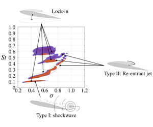
  $\unicode[STIX]{x1D70E}$. Lock-in is observed to occur on the stiff hydrofoil (a) between the Type IIa mode and the first structural sub-harmonic (
 $f_{n}/2$) at
  $\unicode[STIX]{x1D70E}=0.70-0.75$, where on the flexible (b), two instances of lock-in are observed. Firstly between the Type IIb mode and the first structural mode (
 $f_{n}$) for
  $\unicode[STIX]{x1D70E}=0.70-0.75$, and secondly at
  $\unicode[STIX]{x1D70E}=0.4$ between the Type I mode and the second structural sub-harmonic (
 $f_{n}/4$). The fully wetted natural frequency of the hydrofoils, shown non-dimensionally,
  $St_{n}$, as a horizontal dashed line, is modulated due to the presence of the vapour cavity reducing the added mass, thereby increasing the natural frequency.

Figure 12. Spectrograms of  $\unicode[STIX]{x1D6FF}/\bar{c}$ for a range of
  $\unicode[STIX]{x1D70E}$ showing the global unsteady behaviour of the bending deformations. Comparison of the stiff (a) and flexible (b) hydrofoils highlights the increased power of structural deformations on the flexible hydrofoil. This causes increased FSI, particularly at points of lock-in. Both hydrofoils exhibit similar trends observed in the
  $C_{N}$ spectrograms with strong interactions with structural modes where the fully wetted natural frequency of the hydrofoils, shown non-dimensionally,
  $St_{n}$, as a horizontal dashed line.

Figure 13. Spectrogram of  $\unicode[STIX]{x1D703}$ for a range of
  $\unicode[STIX]{x1D70E}$ on the flexible hydrofoils shows similar trends observed in both the
  $C_{N}$ and
  $\unicode[STIX]{x1D6FF}/\bar{c}$ spectrograms with evidence of the Type I, IIa and IIb shedding modes. The highest power occurs at the lock-in frequency of
  $St=0.45$ for
  $\unicode[STIX]{x1D70E}=0.7$ with the fully wetted natural frequency of the hydrofoils, shown non-dimensionally,
  $St_{n}$, as a horizontal dashed line. Significant power is also observed during lock-in at
  $St=0.11$ for
  $\unicode[STIX]{x1D70E}=0.4$.

Figure 14. Comparison of the  $C_{N}$ spectrograms between the stiff (blue) and flexible (red) hydrofoils for
  $C_{N}$ PSD values greater than a threshold of
  $0.2\times 10^{-5}$. The
  $St$ –
  $\unicode[STIX]{x1D70E}$ relationship is seen to be similar between either hydrofoil for the Type I and IIa shedding modes. Differences are observed for the Type IIb shedding mode due to its susceptibility to structural deformations which are largest towards the tip.
The  $C_{N}$ spectrogram of the flexible hydrofoil (figure 11b) reveals the same 3 primary cavity shedding modes observed on the stiff hydrofoil (figure 11a). These include the shockwave-driven Type I mode and the re-entrant-driven Type IIa and IIb modes along with structural excitations. The Type IIa mode is the primary re-entrant jet-driven shedding mode whereas the Type IIb mode refers to the formation of a second cell in the lower portion of the hydrofoil while Type IIa is confined to the upper portion, which are evident via the SPOD and phase plots shown in figure 17. Comparing the key spectral characteristics (figure 14), there exist several similarities, however, there are significant variations between the two hydrofoils due to the increased FSI of the flexible hydrofoil.
Both hydrofoils are seen to exhibit no significant spectral excitation in either  $C_{N}$ or
  $\unicode[STIX]{x1D6FF}/\bar{c}$ for
  $\unicode[STIX]{x1D70E}\geqslant 1.1$. This is despite the flexible hydrofoil experiencing cavity lengths greater than those encountered on the stiff hydrofoil where significant spectral excitation is observed at
  $\unicode[STIX]{x1D70E}=1.0$. SPOD intensity maps for the flexible hydrofoil in figure 17 show high activity for
  $St=0.607$ occurring at mid-span for
  $\unicode[STIX]{x1D70E}=1.0$ linked to re-entrant jet-driven shedding that is of too small of a scale to significantly excite the hydrofoil. For
  $\unicode[STIX]{x1D70E}$ below 1.0, the re-entrant jet instability causes the shedding of clouds on a sufficient scale (Type IIa mode) to excite both hydrofoils with the flexible hydrofoil shedding at a slightly lower frequency of
  $St=0.48$ compared to 0.51 on the stiff at
  $\unicode[STIX]{x1D70E}=0.9$ (figure 15b). The difference in frequency is attributed to the longer cavity on the flexible hydrofoil (figure 8) increasing the duration of each cycle brought about by induced twist deformations. The decrease in
  $\unicode[STIX]{x1D70E}$ from 1.0 to 0.9 also sees a significant increase in both
  $C_{N}$ and
  $\unicode[STIX]{x1D6FF}/\bar{c}$ PSD, with the
  $C_{N}$ PSD increasing two orders of magnitude with the stiff hydrofoil exhibiting the same trend. This shedding mode has the potential to be two-way FSI should cavity volume oscillations become large. However, in this case, the shed vapour cavities are small, limiting the response of the hydrofoil to one-way FSI i.e. small vibrations/deformations forced by the global flow field drive small-scale cavity length modulation.

Figure 15. The  $C_{N}$ PSD for both the stiff and flexible hydrofoils at key values of
  $\unicode[STIX]{x1D70E}$. The spectra show the shedding modes shift frequency as
  $\unicode[STIX]{x1D70E}$ varies with the modes annotated using the labels from table 4. The lock-in phenomenon is evident in both hydrofoils with large amplification of
  $C_{N}$ at
  $\unicode[STIX]{x1D70E}=0.7$ and
  $0.4$. Lock-in occurs when the excitation frequency from the shedding matches either the natural frequency (dashed lines) itself, or one of its harmonics. Note the change in the order of magnitude between each plot.

Figure 16. The  $\unicode[STIX]{x1D6FF}/\bar{c}$ PSD for both the stiff and flexible hydrofoils at key values of
  $\unicode[STIX]{x1D70E}$. The spectra show the shedding modes modulate as
  $\unicode[STIX]{x1D70E}$ varies with the modes annotated using the labels from table 4. Lock-in of the shedding events with either the natural frequency (dashed lines) or the harmonics of the hydrofoils evident, particularly on the flexible hydrofoil at
  $St=0.44$ and
  $0.11$ for
  $\unicode[STIX]{x1D70E}=0.7$ and
  $0.4$, respectively, due to its lower stiffness. Note the change in the order of magnitude between each plot.
As  $\unicode[STIX]{x1D70E}$ is reduced to 0.8, both the
  $C_{N}$ and
  $\unicode[STIX]{x1D6FF}/\bar{c}$ spectra exhibit a dominant peak that matches the fully wetted natural frequency of the flexible hydrofoil, at
  $St=0.40$, while the
  $\unicode[STIX]{x1D6FF}/\bar{c}$ spectrum features a secondary peak at
  $St=0.47$. The lower frequency is associated with the Type IIa shedding of cavitation clouds in the upper portion of the span (
 $0.1\leqslant y/b\leqslant 0.4$), with the
  $St=0.45$ oscillation in the
  $\unicode[STIX]{x1D6FF}/\bar{c}$ linked to Type IIb shedding in the lower portion of the span (
 $0.55\leqslant y/b\leqslant 0.85$), as evident in the SPOD energy maps in figure 17. The formation of two shedding sites matches that observed with the stiff hydrofoil, however, the Type IIb mode occurred at a higher frequency on the stiff hydrofoil at the sane
  $\unicode[STIX]{x1D70E}$ because of shorter cavities. Interestingly, comparison of the hydrofoil’s
  $C_{N}$ spectra at
  $\unicode[STIX]{x1D70E}=0.8$ reveals the absence of any clear Type IIb excitation on the flexible hydrofoil despite being evident on the stiff. This shows signs of significant FSI towards the tip of the flexible hydrofoil. The relatively large tip deformations appear to be interfering with the manifestation of induced hydrofoil loading from shedding cloud cavitation where compliance of the flexible hydrofoil appears to be having the influence of dampening higher-frequency oscillations.

Figure 17. Spectral POD intensity (red) and phase maps (coloured) of key modes for various  $\unicode[STIX]{x1D70E}$ highlighting regions of high activity at the frequencies of interest. The colour intensity distribution in each phase map is directly proportional to that of the corresponding intensity map. The spectral and spatial information aids in the identification of the mechanisms driving oscillations with phase maps providing the relative timing of each cycle.
When reducing  $\unicode[STIX]{x1D70E}$ further to 0.76, there is a shift in the Type IIa shedding frequency down to
  $St=0.31$ with a similar frequency step change observed on the stiff hydrofoil, as seen in figure 11. As mentioned in Part 1, this step change is due to the hydrofoil reaching lock-in where an excitation frequency close enough to the structure’s natural frequency shifts to match this natural frequency, leading to significant amplification of forces and deflections. The Type IIb mode becomes clearly evident on the flexible hydrofoil, exhibiting high amplitude not just in the
  $\unicode[STIX]{x1D6FF}/\bar{c}$ spectra, but in the
  $C_{N}$ and
  $\unicode[STIX]{x1D703}$ spectra as well, shown in figures 11 and 13, respectively. With the Type IIa and IIb frequencies remaining constant as
  $\unicode[STIX]{x1D70E}$ is decreased further to 0.7, significant amplification occurs in both the
  $C_{N}$ and
  $\unicode[STIX]{x1D6FF}/\bar{c}$ spectral peaks with an order of magnitude increase (figure 15e). This is due to the lock-in phenomenon occurring with one of the shedding frequencies locking-in to one of the natural frequencies of the cavitating hydrofoil, causing resonance.
As shown in Part 1, the stiff hydrofoil experiences lock-in for  $0.7\leqslant \unicode[STIX]{x1D70E}\leqslant 0.75$ where the Type IIa root-shedding frequency closely matched the first sub-harmonic of the natural frequency,
  $f_{n}/2$, with added mass considerations, causing maxima in
  $C_{N}^{\prime }$ and
  $\unicode[STIX]{x1D6FF}^{\prime }/\bar{c}$. However, the Type IIa frequency does not match the first sub-harmonic in the case of the flexible hydrofoil. With a lower natural frequency compared to the stiff hydrofoil, the flexible hydrofoil instead experiences lock-in with between the Type IIb oscillations at
  $St=0.45$, with the first natural frequency,
  $f_{n}$, with added mass considerations. This lock-in phenomenon is clearly evident in figures 11(b), 12(b) and 13 with defined high amplitude regions at the lock-in frequency for
  $C_{N}$,
  $C_{P}$,
  $\unicode[STIX]{x1D6FF}/\bar{c}$ and
  $\unicode[STIX]{x1D703}$ along local peaks in
  $C_{N}^{\prime }$,
  $C_{P}^{\prime }$,
  $\unicode[STIX]{x1D6FF}^{\prime }/\bar{c}$ and
  $\unicode[STIX]{x1D703}^{\prime }$ (figure 9). Comparison of the
  $C_{N}$ spectrograms in figure 14 shows how the Type IIb mode locks-in on the flexible hydrofoils structural response with the excitation frequency remaining constant as
  $\unicode[STIX]{x1D70E}$ varies, where in comparison the Type IIb frequency reduces with
  $\unicode[STIX]{x1D70E}$ on the stiff hydrofoil. Lock-in with the Type IIb shedding is also shown in the SPOD maps where energy is concentrated in the lower half of the span for
  $St=0.46$. The lower spectral content observed at higher frequencies in the flexible hydrofoil
  $C_{N}$ spectra compared to that of the stiff is linked to the higher structural damping associated with the composite hydrofoil.
The flexible hydrofoil shifts out of lock-in conditions as  $\unicode[STIX]{x1D70E}$ is decreased down to 0.6 with the Type IIa shedding frequency stepping down to
  $St=0.21$ from 0.45 at
  $\unicode[STIX]{x1D70E}=0.71$. The reduction in
  $\unicode[STIX]{x1D70E}$ sees the Type IIb mode decay significantly in the
  $C_{N}$ spectra while a tonal peak emerges at
  $St=0.46$ particularly evident in the
  $\unicode[STIX]{x1D6FF}/\bar{c}$ spectra, as shown in figure 15(f);
  $\unicode[STIX]{x1D70E}=0.61$ corresponds to the point that the attached cavity now extends slightly downstream of the trailing edge,
  $x_{cop}$ has reached its maximum and the deformed hydrofoil possesses its most negative
  $\bar{\unicode[STIX]{x1D6FC}}_{e}$ with
  $\unicode[STIX]{x1D703}=-0.5^{\circ }$.
The shedding behaviour on the flexible hydrofoil at  $\unicode[STIX]{x1D70E}=0.6$ resembles that of the stiff hydrofoil on the comparison of the SPOD energy maps at each respective Type IIa shedding frequency (figure 17). The high intensity region at the trailing edge extends the majority of the span for approximately
  $St=0.226$ where the phase maps show the upper and lower halves to be out of phase. This indicates that the Type IIa and IIb modes are oscillating at the same frequency where the shed clouds alternate between the upper and lower portions of the span.
The Type IIa shedding frequency continues to reduce steadily at the same rate as the stiff hydrofoil with the attached cavity continuing to grow, showing a linear dependence on  $\unicode[STIX]{x1D70E}$ before disappearing for
  $\unicode[STIX]{x1D70E}<0.4$, as shown in figure 11. The reduction of
  $\unicode[STIX]{x1D70E}$ below 0.6 also shows the emergence of the Type I mode at
  $St=0.11$ as observed on the stiff while remaining nominally independent of
  $\unicode[STIX]{x1D70E}$. As mentioned in Part 1, the emergence of the Type I mode coincides with the attached cavity reaching the trailing edge (figure 8) and is attributed to the presence of the shockwave instability. The SPOD energy maps at
  $\unicode[STIX]{x1D70E}=0.5$ show that at the Type I frequency of
  $St=0.113$, the shedding activity is concentrated along the trailing edge for the majority of the span with the phase map indicating uniform detachment (figure 17). In comparison, the Type IIa mode oscillations at
  $St=0.188$ appear to be concentrated towards the mid-span of the hydrofoil with an isolated region towards the tip forming due to interaction between the cavity and the spanwise tip flow.
The amplitude of the Type I peak in both the  $C_{N}$ and
  $\unicode[STIX]{x1D6FF}/\bar{c}$ spectra starts growing rapidly and earlier compared to the stiff as
  $\unicode[STIX]{x1D70E}$ is reduced as shown in the
  $C_{N}$,
  $\unicode[STIX]{x1D6FF}/\bar{c}$ and
  $\unicode[STIX]{x1D703}$ spectrograms (figures 11, 12 and 13). This leads to the Type I spectral peaks far exceeding the Type IIa peaks at
  $\unicode[STIX]{x1D70E}=0.50$, unlike on the stiff (figures 15g and 16). This is followed by a twofold increase in the Type I peak as
  $\unicode[STIX]{x1D70E}$ is reduced further to 0.41 (figure 15g) with the amplitude on the flexible hydrofoil far exceeding that of the stiff while maintaining a shedding frequency of
  $St=0.11$. The high amplitude of the spectral peak is because the Type I cavity shedding frequency matched with a subharmonic of the first natural frequency,
  $f_{n}/4$, of the flexible hydrofoil;
  $\unicode[STIX]{x1D70E}=0.4$ also coincides with the point of maximum
  $C_{N}^{\prime }$ and
  $\unicode[STIX]{x1D6FF}^{\prime }/\bar{c}$ (figure 9), as well as the normal force and tip deflection being significantly out of phase linked to dampening.
Further reduction in  $\unicode[STIX]{x1D70E}$ to 0.3 sees the Type I mode decays quickly for the flexible hydrofoil with the peak amplitude continuing to grow on the stiff hydrofoil and exceeding the power of the flexible (figure 15). This is an indication of the flexible hydrofoil entering the supercavitation regime where the cavity is starting to extend far enough downstream to prevent the shockwave instability from forming and causing break-off. This is supported by the
  $\unicode[STIX]{x1D70E}=0.30$ SPOD intensity maps in figure 17, where decreased intensity and definition in comparison to the Type I mode at
  $\unicode[STIX]{x1D70E}=0.41$ is observed as the hydrofoil transitions to supercavitation. The earlier transition from the cloud cavitation to supercavitation regime can be linked to the longer cavity on the flexible hydrofoil clearly evident at
  $\unicode[STIX]{x1D70E}=0.4$ and still evident at
  $\unicode[STIX]{x1D70E}=0.3$.
As observed on the stiff hydrofoil, the shockwave-driven Type I mode is no longer apparent on the flexible hydrofoil as  $\unicode[STIX]{x1D70E}$ is reduced to 0.2 with the flow conditions fully shifting the hydrofoil into the supercavitating regime (figure 7). The
  $C_{N}$ spectrogram (figure 11b) shows minimal excitation with no tonal peaks as the hydrofoil no longer experiences large-scale shedding with the cavity closing far downstream, preventing shockwave instabilities from forming. All cavity dynamics with observations made from the forces and deflections for each cavitation regime is discussed in § 3.4.
3.4 Cavity dynamics
3.4.1 Sheet cavitation
Sheet cavitation is experienced by the flexible hydrofoil at high  $\unicode[STIX]{x1D70E}$ as observed on the stiff albeit only intermittently and limited to
  $\unicode[STIX]{x1D70E}=1.2$. From the cavity dynamics analysis of the stiff hydrofoil, there is little to no evidence of re-entrant jet formation with cavity break-up primarily driven by interfacial instabilities for
  $1.1\leqslant \unicode[STIX]{x1D70E}\leqslant 1.2$, as illustrated in figure 18. In comparison, the driver of cavity break-up is observed to interchange between interfacial instabilities and re-entrant jet formation over time on the flexible hydrofoil. This is shown in the spanwise space–time plot for
  $\unicode[STIX]{x1D70E}=1.1$ taken at
  $x/c_{root}=0.31$ (figure 18b) where manifestations of the re-entrant jet are temporarily evident for
  $0\leqslant t^{\prime }\leqslant 3$ and
  $9\leqslant t^{\prime }\leqslant 18$. This indicates that the flexible hydrofoil is in the transition region between sheet cavitation and cloud cavitation.
The acceleration of the transition from sheet to cloud cavitation on the flexible hydrofoil as  $\unicode[STIX]{x1D70E}$ is reduced is associated with the induced
  $\unicode[STIX]{x1D703}$ deformations increasing
  $\bar{\unicode[STIX]{x1D6FC}}_{e}$. The resulting lower pressure on the suction side of the hydrofoil causes the larger attached cavity to grow into a region of increased adverse pressure gradient that allows a re-entrant jet to form and cause shedding. Influence of the
  $\unicode[STIX]{x1D703}$ deformation is taken into account with the cavitation parameter
  $\unicode[STIX]{x1D70E}/2\bar{\unicode[STIX]{x1D6FC}}_{e}$, where at
  $\unicode[STIX]{x1D70E}=1.2$, the stiff and flexible hydrofoils have values of 5.89 and 5.43, respectively. These drop to 5.33 and 4.96 as
  $\unicode[STIX]{x1D70E}$ is reduced to 1.1 for the stiff and flexible hydrofoils, respectively. This suggests more similar cavity dynamics should be observed between the hydrofoils when comparing
  $\unicode[STIX]{x1D70E}=1.1$ on the stiff hydrofoil with
  $\unicode[STIX]{x1D70E}=1.2$ on the flexible, which is observed to be reasonable.

Figure 18. Spanwise space–time plots representing sheet cavitation just prior to a regime transition with reducing  $\unicode[STIX]{x1D70E}$ of the stiff hydrofoil (a) taken at
  $x/c_{root}=0.35$ and
  $\unicode[STIX]{x1D70E}=1.1$ as well as the flexible hydrofoil (b) taken at
  $x/c_{root}=0.31$ and
  $\unicode[STIX]{x1D70E}=1.2$. Where the stiff hydrofoil is seen to experience cavity break-up solely driven by interfacial instabilities, the flexible hydrofoil shows intermittent manifestations of re-entrant jet formation as it is closer to cloud cavitation transition.
3.4.2 Re-entrant jet-driven shedding  $(\text{pre-lock-in})$

As described in Part 1, cloud cavitation occurs when reduction in  $\unicode[STIX]{x1D70E}$ results in the formation of a re-entrant jet that has the ability to reach the upstream extent of the attached cavity, causing periodic cavity detachment. This occurs earlier on the flexible hydrofoil with reducing
  $\unicode[STIX]{x1D70E}$ due to the flow-induced deformations with the onset of cloud cavitation evident at approximately
  $\unicode[STIX]{x1D70E}=1.1$ compared to 1.0 on the stiff hydrofoil.
The early stages of Type IIa re-entrant jet-driven cloud cavitation appears similar for both hydrofoils with each exhibiting a rise in force fluctuations,  $C_{N}^{\prime }$ and
  $C_{P}^{\prime }$ (figure 9) with the shift into the cloud cavitation regime. Analysis of the cavitation behaviour on each hydrofoil at
  $\unicode[STIX]{x1D70E}=1.0$ (figure 19) shows the re-entrant jet mechanism confined to around mid-span due to three-dimensional flows effects mentioned in Part 1. Comparison of the space–time plots shows different frequencies with the stiff experiencing a slightly higher shedding frequency at
  $St=0.74$ compared to
  $St=0.61$ on the flexible which can be linked to the difference in
  $\unicode[STIX]{x1D70E}/2\bar{\unicode[STIX]{x1D6FC}}_{e}$ and cavity length.

Figure 19. Spanwise space–time plots showing cloud cavitation of the stiff (a) and flexible (b) hydrofoils taken at  $x/c_{root}=0.31$ and
  $x/c_{root}=0.35$, respectively, for and
  $\unicode[STIX]{x1D70E}=1.0$. The re-entrant jet remains confined to around mid-span due to three-dimensional effects on each hydrofoil. The stiff hydrofoil exhibits a slightly higher shedding frequency of
  $St=0.74$ compared to
  $St=0.61$ on the flexible which is linked to induced
  $\unicode[STIX]{x1D703}$ angle increasing
  $\unicode[STIX]{x1D70E}/2\bar{\unicode[STIX]{x1D6FC}}_{e}$ and cavity length.
As  $\unicode[STIX]{x1D70E}$ is decreased further down to 0.8,
  $x_{cop}$ shifts downstream where it lies close to the elastic axis, resulting in minimal twist deformations and therefore similar conditions for the stiff and flexible hydrofoils. As observed on the stiff hydrofoil, the reduction in
  $\unicode[STIX]{x1D70E}$ sees the cavity along with the re-entrant jet thickness grow, giving the re-entrant jet enough momentum to overcome spanwise flow components and reach the leading edge for majority of the span (figure 20). This growth in the attached cavity and inherent cavity dynamics results in spatial compatibility with the hydrofoil where a secondary shedding mode appears on each hydrofoil, the Type IIb shedding mode. The formation of two defined shedding cells is clearly evident on the stiff hydrofoil as discussed in Part 1 and shown in figure 20(b), but not as defined on the flexible hydrofoil (figure 20d).
Analysis of the space–time plot in figure 20(d) shows strong periodic shedding of the Type IIa mode at  $St=0.41$ in the upper portion, although large re-entrant jet shedding events are evident around mid-span not observed on the stiff hydrofoil. Comparison of the cavitation pattern in the lower portion of the span highlights the higher degree of cavity break-up on the flexible hydrofoil compared to the stiff hydrofoil, making shedding events unclear, particularly at
  $8\leqslant t^{\prime }\leqslant 13$. This period is seen to correspond to an interval of low structural deformations in both
  $\unicode[STIX]{x1D6FF}/\bar{c}$ and
  $\unicode[STIX]{x1D703}$ (figure 9), indicating a strong FSI influence. The induced deformations and vibrations from the fluctuating loads appear to be disrupting the cavity dynamics and inhibiting cavity formation particularly towards the tip were deformations are large.

Figure 20. Both hydrofoils experience the formation of two shedding sites along the span at  $\unicode[STIX]{x1D70E}=0.8$ due to the spatial compatibility between the attached cavity and the planform geometry. This is shown by the spanwise space–time plots taken at
  $x/c_{root}=0.5$ and
  $0.58$ for the stiff (b) and flexible (d) hydrofoils, respectively. However, the real value
  $C_{N}$ Morlet wavelet transform from the stiff hydrofoil (a) shows the multi-modal behaviour at
  $St=0.41$ (purple horizontal line) and
  $0.50$ (green horizontal line), while for the flexible hydrofoil (c), only the
  $St=0.40$ (purple horizontal line) Type IIa mode is evident in the wavelet transform. Closer inspection of the cavitation behaviour towards the tip shows a higher degree of break-up on the flexible hydrofoil compared to the stiff, linked to the larger deformations.
3.4.3 Lock-in
As observed on the stiff hydrofoil in Part 1, the flexible hydrofoil experiences the lock-in phenomenon where the shedding frequency locks-in to a structural mode of the hydrofoil that leads to amplification of small motions and fluctuating fluid loads (Harwood et al. Reference Harwood, Felli, Falchi, Garg, Ceccio and Young2019). The flexible hydrofoil starts to experience lock-in with the reduction in  $\unicode[STIX]{x1D70E}$ down to 0.75 where we see the Type IIb tip shedding frequency lock-in to the first mode of the hydrofoil at
  $St=0.44$ in figures 11–14. This is a slightly higher frequency than that in fully wetted conditions (
 $St=0.38$) due to reduced added mass caused by phase change from water to vapour on the cavitation portions of the hydrofoil. Experimental measurements quantifying the change in added mass and modal frequencies with cavitation and ventilation can be found in Harwood et al. (Reference Harwood, Felli, Falchi, Garg, Ceccio and Young2020). Lock-in differs between hydrofoils with the stiff experiencing lock-in between the first sub-harmonic of the structure and the Type IIa shedding due to the increased stiffness and lower added mass sensitivity. With lock-in occurring between the tip shedding mode and the first structural mode, increased FSI is observed for the flexible hydrofoil with the inherently higher deflections in the lower span.
The severity of lock-in is increased as  $\unicode[STIX]{x1D70E}$ is reduced further to 0.7 where the hydrofoil is observed to experience the largest
  $\unicode[STIX]{x1D703}$ fluctuations, along with local peaks in
  $C_{N}^{\prime }$,
  $\unicode[STIX]{x1D6FF}^{\prime }/\bar{c}$ (figure 9). Lock-in at
  $\unicode[STIX]{x1D70E}=0.7$ on the flexible hydrofoil has more influence on the deformations compared to the stiff hydrofoil which has more influence on forces. This is due to the location of the lock-in shedding modes with the root shedding Type IIa mode occurring in a region of longer chord where the proximity of the Type IIb mode to the free tip increases the influence on deformations. This is highlighted in figures 15 and 16 with the difference between the Type IIa and IIb amplitudes in the
  $C_{N}$ and
  $\unicode[STIX]{x1D6FF}/\bar{c}$ spectra for each hydrofoil.
Comparison of the time series at  $\unicode[STIX]{x1D70E}=0.7$ for the stiff hydrofoil in figure 21(a–c) and the flexible hydrofoil in figure 21(d–g) highlights the difference due to FSI effects. The lock-in of the first natural frequency of the flexible hydrofoil with the Type IIb shedding is exhibited in the
  $C_{N}$ wavelet (figure 21e,f) where a more consistent and strong component is shown at
  $St=0.44$ compared to
  $St=0.49$ on the stiff (figure 21a,b). The strong interaction of the tip shedding with twist deformations is also exhibited in the
  $\unicode[STIX]{x1D703}$ time series exhibiting a strong
  $St=0.44$ fluctuation in figure 21. Interestingly, comparison of the tip displacement time series shows a similar range of oscillation despite the significant difference in stiffness, indicating twist deformations to be the primary influence on the cavity dynamics. These structural deformations translate into defined and consistent tip shedding events, as shown in figure 21(g), particularly when compared to the stiff in figure 21(c). Despite tip shedding events being more defined in the flexible space–time plot, the cavity appears more broken and dispersed compared to the stiff, particularly towards the tip and downstream end of the cavity. This is attributed to the increased FSI from the structural deformation disrupting the growth and stability of the attached cavity.

Figure 21. The multi-modal behaviour on either hydrofoil is shown in plots of the real values of Morlet wavelet transforms for  $C_{N}$ (a (stiff), e (flexible)) at
  $\unicode[STIX]{x1D70E}=0.7$. Extracting the Type IIa and IIb wavelet components at
  $St=0.29$ and
  $0.49$ for the stiff hydrofoil (b) and
  $St=0.30$ and
  $0.44$ for the flexible hydrofoil (f), respectively, shows the correlation with shedding events. These shedding events along the span are evident in the spanwise space–time plots taken at
  $x/c_{root}=0.5$ and
  $0.58$ for the stiff (c) and flexible (g) hydrofoils, respectively.
3.4.4 Re-entrant jet-driven shedding (post-lock-in)
The flexible hydrofoil comes out of lock-in with enough reduction in  $\unicode[STIX]{x1D70E}$ down to 0.65 with fluctuations in both forces and deflections decreasing, as shown in figure 9. The transition out of lock-in is also made evident in the
  $C_{N}$ and
  $\unicode[STIX]{x1D6FF}/\bar{c}$ spectra (figures 15 and 16) where amplification of the forces and deflection is no longer evident, leading to decreased interaction between the cloud cavitation and structural deformations. The decrease in
  $\unicode[STIX]{x1D70E}$ leads to a larger cavity that now reaches the trailing edge of the hydrofoil (i.e.
  $L_{c}/c=1.0$). This increased length results in a cavity that no longer has spanwise spatial compatibility for two cells to form, leading to the disappearance of the Type IIb mode, as observed on the stiff hydrofoil.
With the cavity reaching the trailing edge, shockwave instabilities become active as the attached cavity extends into the high pressure region downstream of the trailing edge. As described in Part 1, small-scale break-up of the cavity from surface perturbations forming as the re-entrant jet moves upstream preconditions the flow for condensation shockwaves to form. Similar to the stiff hydrofoil, the shockwave causes the shedding of cloud cavitation where the re-entrant jet instability drives the frequency. However, due to increased FSI, the emergence of the shockwave instability is accelerated on the flexible hydrofoil with similar behaviour seen between the stiff hydrofoil at  $\unicode[STIX]{x1D70E}=0.6$ and the flexible at
  $\unicode[STIX]{x1D70E}=0.65$, as shown in figure 22.

Figure 22. Synchronised time series of the normal force ( $C_{N}$) and tip displacement (
 $\unicode[STIX]{x1D6FF}/\bar{c}$) (a (stiff), d (flexible)) along with the flexible hydrofoils pitching moment and twist (
 $\unicode[STIX]{x1D703}$) (f) at
  $\unicode[STIX]{x1D70E}=0.60$ and
  $0.65$ for the stiff and flexible hydrofoils, respectively. The real value of the Morlet wavelet transforms for
  $C_{N}$ (b (stiff), e (flexible)) shows the intermittent behaviour of shedding modes, also being evident in the space–time plots for the stiff (c) and flexible (g) hydrofoils taken at
  $x/c_{root}=0.5$ and
  $0.58$, respectively.
Further reduction in  $\unicode[STIX]{x1D70E}$ down to 0.55 sees the Type IIa shedding frequency decrease linearly to
  $St=0.20$ with the growth in cavity length resulting in partially coherent shedding along the span. As observed on the stiff hydrofoil at
  $\unicode[STIX]{x1D70E}=0.5$, shedding along the span consists of several shedding events starting near the root and then occurring successively out along the span. This is evident in both space–time plots (figure 23c–e) by the 3–4 breaks in the cavitation pattern per cycle. The similarity between the cavitation behaviour and frequencies suggests that the hydrofoils should possess similar
  $\unicode[STIX]{x1D70E}/2\bar{\unicode[STIX]{x1D6FC}_{e}}$ at
  $\unicode[STIX]{x1D70E}=0.5$ and
  $0.55$ for the stiff and flexible, respectively, with
  $\unicode[STIX]{x1D703}$ increasing
  $\bar{\unicode[STIX]{x1D6FC}_{e}}$. However, the flexible hydrofoil deformations result in
  $\unicode[STIX]{x1D703}=-0.5^{\circ }$, resulting in a significantly higher
  $\unicode[STIX]{x1D70E}/2\bar{\unicode[STIX]{x1D6FC}_{e}}$ value of 2.78, compared to 2.41.
Comparison of the synchronised force and deflection time series, along with the space–time plots in figure 23 highlights a more complex cavitation behaviour on the flexible hydrofoil compared to the stiff. With both the re-entrant jet and shockwave instability being active while neither dominates the physics, the shedding behaviour varies through time. This was highlighted in Part 1 with the stiff hydrofoil at  $\unicode[STIX]{x1D70E}=0.4$ where the Type I mode was shown not to be continuously apparent through time in a long duration time series. This non-stationary multi-modal behaviour is shown in the flexible hydrofoils
  $C_{N}$ wavelet at
  $\unicode[STIX]{x1D70E}=0.55$ (figure 23c) where a transition from the Type IIa mode to the Type I mode is apparent in the range
  $15\leqslant t^{\prime }\leqslant 25$, highlighting the need for time–frequency analysis. This transition is also evident in the
  $\unicode[STIX]{x1D703}$ time series where a
  $St\approx 0.53$ oscillation fades out at
  $t^{\prime }\approx 15$ before a
  $St\approx 0.25$ oscillation appears at
  $t^{\prime }\approx 25$, coinciding with the transition between modes shown in the
  $C_{N}$ wavelet.

Figure 23. With several shedding mechanisms and modes active on each hydrofoil at a certain  $\unicode[STIX]{x1D70E}$, the interactions and role of FSI becomes complex. At
  $\unicode[STIX]{x1D70E}=0.5$ on the stiff hydrofoil, the
  $C_{N}$ wavelet (a) shows the Type I (
 $St=0.11$) and IIa (
 $St=0.19$) modes being simultaneously active. Power of the Type I mode can be seen growing with
  $t^{\prime }$ in the
  $C_{N}$ wavelet (a), corresponding with a change in the cavity physics evident in the spanwise space–time (b) taken at
  $x/c_{root}=0.58$. This multi-modal behaviour is also observed on the flexible hydrofoil at
  $\unicode[STIX]{x1D70E}=0.55$ where a clear transition in the
  $C_{N}$ wavelet (c) is evident from the Type II mode (
 $St=0.20$) to the Type I mode (
 $St=0.11$) at
  $t^{\prime }=20$. This transition is also evident in the
  $\unicode[STIX]{x1D703}$ deformations (d) with oscillations shifting from high to low, as well as in the cavity dynamics where the spanwise space–time plot (e) at
  $x/c_{root}=0.65$ shows larger cavitation clouds being shed along the span when the Type I mode is active.

Figure 24. Synchronised time series of the normal force ( $C_{N}$) and tip displacement (
 $\unicode[STIX]{x1D6FF}/\bar{c}$) (a (stiff), d (flexible)) along with the flexible hydrofoil pitching moment and twist (
 $\unicode[STIX]{x1D703}$) (f) at
  $\unicode[STIX]{x1D70E}=0.4$ and
  $0.5$ for the stiff and flexible hydrofoils, respectively. The real value of the Morlet wavelet transforms for
  $C_{N}$ (b (stiff), e (flexible)) shows the different dominant modes of either hydrofoil, also evident in the space–time plots for the stiff (c) and flexible (g) hydrofoils both taken at
  $x/c_{root}=0.5$.
3.4.5 Shock-wave-driven shedding
As mentioned previously, the shockwave instability first becomes apparent at  $\unicode[STIX]{x1D70E}=0.6$ on the flexible hydrofoil, just as the attached cavity reaches the trailing edge, i.e.
  $L_{c}/c=1.0$. Unlike on the stiff hydrofoil, the impact of the shockwave increases quickly as
  $\unicode[STIX]{x1D70E}$ is reduced, with the Type I mode dominating the
  $C_{N}$ and
  $\unicode[STIX]{x1D6FF}/\bar{c}$ spectra (figures 15 and 16) by the point
  $\unicode[STIX]{x1D70E}$ reaches 0.5. In comparison, the stiff hydrofoil spectrum is still dominated by the Type IIa mode down to
  $\unicode[STIX]{x1D70E}=0.4$;
  $\unicode[STIX]{x1D70E}=0.4$ and
  $\unicode[STIX]{x1D70E}=0.5$ for the stiff and flexible, respectively, have been chosen for comparison in figure 24 due to the similarity of shedding modes and amplitudes. The dominance by the Type IIa mode is highlighted in the synchronised time series where the stiff hydrofoil
  $C_{N}$ wavelet (figure 24b) is dominated by the Type IIa mode at
  $St=0.16$. On the other hand, for the flexible hydrofoil, with the Type IIa mode still being present, the Type I mode dominates the time series at
  $St=0.11$ for
  $\unicode[STIX]{x1D70E}=0.5$ (figure 24e). In addition, a phase lag becomes apparent between
  $C_{N}$ and
  $\unicode[STIX]{x1D6FF}/\bar{c}$ in the synchronised time series (figure 24d) with a phase difference of approximately
  $\unicode[STIX]{x03C0}/4$.
Comparing the spanwise space–time plots of the stiff and flexible hydrofoils at  $\unicode[STIX]{x1D70E}=0.4$ and 0.5, respectively, provides insight into the cavity physics driving the forces and deformations. As mentioned in Part 1, the stiff hydrofoil experiences alternate shedding between the upper and lower spans, as shown in figure 24(c), driven by the re-entrant jet instability. On the other hand, shedding is more uniform along the flexible hydrofoil span, resulting in increased forces and deflections from larger shed cavities breaking off at
  $St=0.11$ (figure 24g). This is highlighted in the SPOD energy maps, where the phase is uniform along the span for
  $\unicode[STIX]{x1D70E}=0.5$ at
  $St=0.11$ (figure 17).
Once the cavity grows to the full chord the void fraction increases, and the sound speed reduces (Shamsborhan et al. Reference Shamsborhan, Coutier-Delgosha, Caignaert and Nour2010), to a point where the flow is susceptible to the shockwave instability. The onset of the shockwave instability at higher cavitation numbers for the flexible case is presumably attributable to the increased compliance and the deformation. These are manifest in both the magnitude and shedding modes as apparent in the space–time diagrams and corresponding force and deflection time series in figure 24. As shown, the shedding modes are not as coherent for the flexible as they are for the stiff, as the stiff space–time diagram shows a regular, alternate, root-tip shedding system, but the flexible case shows coupled root-tip shedding with intermittent two-dimensional shedding events, showing the effect of compliance on the shedding topology. The increased amplitude of  $C_{N}$ is due to the lock-in phenomenon described earlier, as evidenced from the associated increased deformations as shown in figures 15(g,h) and 16(g,h). The fluid mechanics associated with shockwave phenomena in cavitating flows are highly complex and influenced by a range of factors that are not all fully understood, with observations varying between similar experiments (Leroux, Astolfi & Billard Reference Leroux, Astolfi and Billard2004; Leroux, Coutier-Delgosha & Astolfi Reference Leroux, Coutier-Delgosha and Astolfi2005). The initiation and modes of propagation of shockwaves have been shown to vary greatly depending on the nature of the flow involved including factors such as the global cavity topology, three-dimensional effects, pressure gradients and the level of nucleation. Observations of high-speed imaging (e.g. supplementary material movie 7 for a cavitation number of 0.5) show shockwaves to mostly be initiated when portions of the growing cavitation reach the local chord. After which, propagation may be in the chordwise direction but also in the spanwise direction. The interaction of these shockwaves due to the tapered planform creates the shedding modes seen in the space–time diagrams, which were discussed in more detail in Part 1. Beyond the differences in compliance, some chordwise streaks are evident in the cavitation for the flexible hydrofoil that are not present for the stiff hydrofoil. These have been found to be due to leading edge imperfections resulting from the composite manufacturing process. It is possible that these streaks could affect cavity dynamics, although with the results available it is difficult to make definitive observations.
Further reduction in  $\unicode[STIX]{x1D70E}$ down to 0.4 on the flexible hydrofoil sees large amplification of both
  $C_{N}$ and
  $\unicode[STIX]{x1D6FF}/\bar{c}$ PSDs at the Type I frequency of
  $St=0.11$, corresponding to the points of maximum
  $C_{N}^{\prime }$ and
  $\unicode[STIX]{x1D6FF}^{\prime }/\bar{c}$ for the flexible hydrofoil for the
  $\unicode[STIX]{x1D70E}$ range tested. Additionally, a phase shift appears between
  $C_{N}$ and
  $\unicode[STIX]{x1D6FF}/\bar{c}$ with the force and deflection becoming out of phase by approximately
  $\unicode[STIX]{x03C0}$ for the flexible hydrofoil in figure 25(c), not observed on the stiff hydrofoil (figure 25a). These phenomena are due to the flexible hydrofoil entering secondary lock-in between the Type I shedding mode and the
  $f_{n}/4$ sub-harmonic. The strong FSI effects involved in lock-in cause both uniform and periodic spanwise shedding of large-scale cavitation clouds that cause enlarged fluctuations in both the forces and deformations. The shift in phase between
  $C_{N}$ and
  $\unicode[STIX]{x1D6FF}/\bar{c}$ fluctuations are linked to a reduction in damping brought about from the sub-harmonic lock-in and the increased cavity size allowing a greater portion of the hydrofoil to oscillate in a vapour cavity as opposed to the fluid.

Figure 25. Synchronised time series of the normal force ( $C_{N}$) and tip displacement (
 $\unicode[STIX]{x1D6FF}/\bar{c}$) at
  $\unicode[STIX]{x1D70E}=0.3$ and
  $0.4$ for the stiff (a) and flexible (c) hydrofoil, respectively. The spanwise space–time plots of the stiff (b) and flexible (d) taken at
  $x/c_{root}=0.5$ show the dominant Type I shedding frequency that correlates well with
  $C_{N}$ and
  $\unicode[STIX]{x1D6FF}/\bar{c}$ time series.
Comparing cavitation behaviour on either hydrofoil at  $\unicode[STIX]{x1D70E}$ values corresponding to solely Type I shockwave-driven shedding reveals several key differences. The shedding cycle on the stiff hydrofoil at
  $\unicode[STIX]{x1D70E}=0.3$ consists of a sequence of shedding events where a large-scale cloud is shed from the upper portion of the span, followed by two medium-scale clouds around mid-span in quick succession (figure 25b). This results in two small peaks in each of the
  $St=0.09$ cycles in both the
  $C_{N}$ and
  $\unicode[STIX]{x1D6FF}/\bar{c}$ time series (figure 25a). As for the flexible hydrofoil, it follows the behaviour observed at
  $\unicode[STIX]{x1D70E}=0.5$ with uniform coherent shedding along the span with the spanwise space–time plot showing clear shockwave-driven cavity break-up (figure 25d). The chordwise space–time plots in figure 26 at the same
  $\unicode[STIX]{x1D70E}$ values show both hydrofoils experiencing the growth, stable and shockwave phases in each shedding cycle, as discussed in Part 1. However, comparing the hydrofoils, the shedding behaviour on the flexible appears more inconsistent in terms of cavity dynamics and cycle duration.

Figure 26. Chordwise space–time plots of the stiff (a) and flexible (b) hydrofoils both taken at  $y/b=0.25$ for
  $\unicode[STIX]{x1D70E}=0.3$ and
  $0.4$, respectively, showing the cavity dynamics for solely Type I shockwave-driven shedding. Both hydrofoils exhibit the growth, stable and shockwave phases for each cycle, however, the flexible hydrofoil exhibits more inconsistent cycles in terms of cavity dynamics and cycle duration.
As  $\unicode[STIX]{x1D70E}$ is reduced down to 0.3, fluctuations in both
  $C_{N}$ and
  $\unicode[STIX]{x1D6FF}/\bar{c}$ reduce as the shockwave instability weakens on the flexible hydrofoil with the phase lag between
  $C_{N}$ and
  $\unicode[STIX]{x1D6FF}$ reducing to approximately
  $\unicode[STIX]{x03C0}/2$. The growth of the cavity has it extending far enough downstream of the hydrofoil into the region that limits the formation of certain instabilities. This results in only a relatively weak shockwave forming, reducing the impact on the forces and deflections but sufficient enough to cause shedding, as shown in figure 27. This stage of shockwave-driven shedding is not observed on the stiff hydrofoil as it occurs at a
  $\unicode[STIX]{x1D70E}$ of approximately 0.25, a point not captured in the short type runs. Further reduction in
  $\unicode[STIX]{x1D70E}$ sees the hydrofoil enter supercavitation, discussed in § 3.4.6.

Figure 27. At  $\unicode[STIX]{x1D70E}=0.3$, the phase lag between
  $C_{N}$ and
  $\unicode[STIX]{x1D6FF}/\bar{c}$ observed for the flexible hydrofoil at
  $\unicode[STIX]{x1D70E}=0.4$ is still evident (a) with the
  $\unicode[STIX]{x1D703}$ deformations (b) seen to be in phase with
  $C_{P}$ at the Type I
  $St=0.10$ frequency. The weakening of the shockwave-driven shedding as the flexible hydrofoil approaches the transition to supercavitation is evident in the spanwise space–time plot (c) taken at
  $x/c_{root}=0.73$ showing minimal cavity break-up.
3.4.6 Supercavitation
The flexible hydrofoil transitions into the supercavitation regime as  $\unicode[STIX]{x1D70E}$ is reduced from 0.3 down to 0.2. As observed on the stiff hydrofoil, the significant growth in the cavity length to
  $L_{c}/c>1.5$ has the cavity closing far downstream where it becomes more stable than a partial cavity as no substantial shedding mechanism can form (figure 7). There is little to no difference between the hydrofoils in terms of forces, deflections and cavitation behaviours as the forces have decreased to a point of little influence compared to the stiffness of the hydrofoil (figure 28). One difference observed between the hydrofoils is the presence of streaks that extend from the upstream extent of the cavity down to the break-up region of the supercavity (figure 7). As discussed previously, these are due to small surface imperfections on the flexible hydrofoil stemming from the composite manufacturing process and are seen to have negligible influence on the supercavitation regime.

Figure 28. Synchronised time series of the normal force ( $C_{N}$) and tip displacement (
 $\unicode[STIX]{x1D6FF}/\bar{c}$) at
  $\unicode[STIX]{x1D70E}=0.2$ for the stiff (a) and flexible (c) hydrofoils. The spanwise space–time plots of the stiff (b) and flexible (d) taken at
  $x/c_{root}=0.75$ show minimal activity in the supercavity as it closes far enough downstream to prevent shedding mechanisms from forming.
4 Conclusion
The influence of FSI on cloud cavitation about a hydrofoil was investigated through comparison of simultaneously acquired high-speed photography and force measurements on stiff and flexible hydrofoils. FSI was observed to influence all cavitation regimes with the flexible hydrofoil seen to experience accelerated cavitation regime transition with reducing  $\unicode[STIX]{x1D70E}$. Hydrodynamic bend–twist coupling is seen to result in nose-up twist deformations on the flexible hydrofoil for
  $\unicode[STIX]{x1D70E}>0.7$, causing an early transition from the sheet cavitation regime into the re-entrant jet-driven cloud cavitation regime at
  $\unicode[STIX]{x1D70E}=1.1$. The nose-up bend–twist coupling has the added effect of increasing the cavity length, resulting in a reduced shedding frequency, particularly evident in the Type IIa mode at higher
  $\unicode[STIX]{x1D70E}$ values. Lock-in occurs on the flexible hydrofoil for
  $0.70\leqslant \unicode[STIX]{x1D70E}\leqslant 0.75$, as observed on the stiff hydrofoil. However, the flexible hydrofoil experiences lock-in between the Type IIb mode and the first structural mode (
 $f_{n}$). Additionally, the flexible hydrofoil appears to attenuate relatively high frequency oscillations with
  $C_{N}$ PSD peaks on the stiff hydrofoil surpassing all those of the flexible for
  $0.6\leqslant \unicode[STIX]{x1D70E}\leqslant 0.9$, despite higher deformations. Despite hydrodynamic bend–twist coupling causing nose-down twist deformations as the centre of pressure shifts downstream of the elastic axis for
  $\unicode[STIX]{x1D70E}\leqslant 0.7$, the flexible hydrofoil still experiences accelerated cavitation regime transition with reducing
  $\unicode[STIX]{x1D70E}$. This is seen with the rapid growth of influence the shockwave instability has on the forces, deflections and cavitation behaviour on the flexible hydrofoil, suggesting the larger dynamic structural behaviour plays a significant role in the cavity physics. As
  $\unicode[STIX]{x1D70E}$ is reduced to 0.4, the different structural properties of the flexible hydrofoil lead to secondary lock-in, this time between the Type I mode and the
  $f_{n}/4$ harmonic. This leads to amplification of structural deformations and forces while also coinciding with a
  $\unicode[STIX]{x03C0}$ shift in phase between
  $C_{N}$ and
  $\unicode[STIX]{x1D6FF}/\bar{c}$ linked to a reduced damping brought about from the increased cavity size allowing a greater portion of the hydrofoil to oscillate in a vapour cavity as opposed to the liquid. Interestingly, this secondary lock-in involving the Type I mode was not observed on the stiff hydrofoil because of the higher first structural frequency. Further reduction in
  $\unicode[STIX]{x1D70E}$ sees the flexible hydrofoil shift out of lock-in at
  $\unicode[STIX]{x1D70E}=0.3$ with signs of supercavitation forming, where in comparison, the stiff hydrofoil still experiences strong shockwave-driven shedding, before both reach supercavitation at
  $\unicode[STIX]{x1D70E}=0.2$. The structurally driven spanwise cavity oscillations observed on the flexible hydrofoil were not observed on the stiff hydrofoil, indicating significant differences in the conditions at the tip. Comparison of the forces, deflections and cavitation behaviour acting on the stiff and flexible hydrofoils shows significant FSI with flexibility leading to high-frequency attenuation of the forces, frequency modulation, accelerated cavitation regime transition as well as multiple lock-in modes.
Acknowledgements
This project was supported by the Research Training Centre of Naval Design and Manufacturing (RTCNDM), the US Office of Naval Research (Dr K.-H. Kim, Program Officer) and ONR Global (Dr W.-M. Lin) through NICOP S&T grant no. N62909-11-1-7013. The RTCNDM is a University–Industry partnership established under the Australian Research Council (ARC) Industry Transformation grant scheme (ARC IC140100003). The authors would like to acknowledge the assistance of Mr S. Kent and Mr R. Wrigley from the Australian Maritime College for their essential help with setting up and carrying out the experiments.
Declaration of interests
The authors report no conflict of interest.
Supplementary movies
Supplementary movies are available at https://doi.org/10.1017/jfm.2020.323.


