


1. Introduction
The structure of turbulent boundary layers developing over rough surfaces has been the object of numerous studies (e.g. see Jimenez Reference Jimenez2004; Castro Reference Castro2007 for a review). One type of rough-bed boundary layers that are particularly relevant for environmental mechanics applications is when the boundary layer develops over sparse larger-scale roughness elements (e.g. irregular arrays of large boulders in mountain rivers). The focus of the present study is on such a type of boundary layers that develop over a bed containing partially burrowed mussels where the protruding parts of the freshwater mussels correspond to the roughness elements. Such large patches/communities/colonies of partially burrowed mussels are referred to as mussel beds. They play a critical role for ecological processes occurring at the water–sediment interface, and affect river dynamics and habitat (Marion et al. Reference Marion2014). A particular feature of this type of rough-bed boundary layers, which are not limited only to rivers but also encountered in marine environments, is that each mussel exchanges mass with the overflow through their syphons, but the net flow exchange is equal to zero. In particular, the excurrent-syphon jet is a source of momentum for the boundary layer. As mussels align with the mean flow and their shells are close to an ellipsoid, their degree of bluntness is much more reduced compared with the typical shapes of the roughness elements (e.g. rectangular cuboids) considered in previous studies of boundary layers developing over arrays of sparse roughness elements (e.g. Yang et al. Reference Yang, Sadique, Mittal and Meneveau2016). Moreover, this type of boundary layers develops in a depth-limited flow, which means that the flow outside of the boundary layer accelerates in the streamwise direction, which is not the case for most types of rough-bed boundary layers investigated in previous experimental and numerical studies. Though the present research is motivated by the need to understand flow structure in rivers containing mussel beds, the main goal of the study is more general and is related to characterising the spatial development of rough-bed boundary layers in depth-limited environments for cases where sparse roughness elements of streamlined shape are present at the bed. The focus of most of the research reported in the literature was on rough-bed boundary layers containing sparse roughness elements with a high degree of bluntness of the roughness elements and on the case where the boundary layer growth is not limited in the vertical direction.
1.1. Background
Freshwater mussels are invertebrates that live on the riverbed substrate with part of their shell being exposed to the water flow. Each mussel contains an excurrent syphon and an incurrent syphon on their posterior side. The discharges through the two syphons are equal at all times. Mussels can vary the flow through their syphons depending on the surrounding flow conditions (e.g. to reduce drag, Di Maio & Corkum Reference Di Maio and Corkum1997). The relative strength of the active filtering is generally characterised by the value of the syphon momentum ratio or filtration velocity ratio, VR, defined as the ratio between the velocity of the flow in the excurrent syphon, Ue , and the bulk channel velocity, U0 (figure 1 a). Using their muscular foot, they can modify their level of burrowing in the substrate. They are generally oriented parallel to the mean flow to reduce drag forces and the probability to be dislocated from the river bed by the overflow.

Figure 1. Computational domain containing the partially burrowed mussels: (a) protruding part of the shell of one mussel showing main geometrical dimensions and bulk velocities through the incurrent and excurrent syphons; (b) positions of the mussels in the simulations conducted with with
 $\rho$
N
$\rho$
N
 $=$
55 mussels m−2, h/d
$=$
55 mussels m−2, h/d
 $=$
0.5; (c) computational mesh in a vertical plane cutting through some of the mussels. The length of the region containing partially burrowed mussels is Lbd
.
$=$
0.5; (c) computational mesh in a vertical plane cutting through some of the mussels. The length of the region containing partially burrowed mussels is Lbd
.
River regions covered by mussel beds are characterised by increased flow resistance, decreased near-bed velocities and increased turbulence away from the bed compared with regions where mussels are very scarce or absent (Nakato, Christensen & Schonhoff Reference Nakato, Christensen and Schonhoff2007; Allen & Vaughn Reference Allen and Vaughn2009; Sansom et al. Reference Sansom, Bent, Atkinson and Vaughn2020; Lazzarin et al. Reference Lazzarin, Constantinescu, Wu and Viero2024). The population density of mussel beds, or the mussel array density,
 $\rho$
N
$\rho$
N
 $=$
N/Abed
(N is the total number of mussels forming the mussel bed whose total surface is Abed
) is generally less than 200 mussels per square metre in rivers (Coco et al. Reference Coco, Thrush, Green and Hewitt2006; Sansom et al. Reference Sansom, Bent, Atkinson and Vaughn2020). Habitat suitability is a strong function of hydrodynamic conditions that are controlling the capacity of mussels to resist dislocation from the substrate. Flow structure over the mussel bed also controls turbulent entrainment of nutrients into the benthic boundary layer (Nakato et al. Reference Nakato, Christensen and Schonhoff2007).
$=$
N/Abed
(N is the total number of mussels forming the mussel bed whose total surface is Abed
) is generally less than 200 mussels per square metre in rivers (Coco et al. Reference Coco, Thrush, Green and Hewitt2006; Sansom et al. Reference Sansom, Bent, Atkinson and Vaughn2020). Habitat suitability is a strong function of hydrodynamic conditions that are controlling the capacity of mussels to resist dislocation from the substrate. Flow structure over the mussel bed also controls turbulent entrainment of nutrients into the benthic boundary layer (Nakato et al. Reference Nakato, Christensen and Schonhoff2007).
One of the most important ecological functions of large communities of mussels is to filter water (Polvi & Sarneel Reference Polvi and Sarneel2018). The filtering rate of mussels depends on the species and mussel dimensions (Monismith et al. Reference Monismith, Koseff, Thompson, O’Riordan and Nepf1990; Bunt, Maclsaac & Sprules Reference Bunt, Maclsaac and Sprules1993). Active filtering was shown to influence local mixing patterns around the mussels (Nishizaki & Ackerman Reference Nishizaki and Ackerman2017), as well as turbulent kinetic energy distribution in the wake (Sansom et al. Reference Sansom, Bent, Atkinson and Vaughn2020). By consuming phytoplankton and zooplankton, mussels reduce the concentration of nitrates in many rivers where high nitrogen content is a cause of great concern for water quality. The interest in understanding how the various ecological functions of mussels and their capacity to survive at the river bed are affected by hydrodynamics motivates the present study that tries to characterise the structure and growth of the boundary layer generated over a mussel bed under different conditions (e.g. mussel array density, level of mussel burrowing, filtering rate). For example, mussels have a larger probability to survive high flow events in rivers if the mussel bed is situated in a region of low bed shear stress (Morales et al. Reference Morales, Weber, Mynett and Newton2006; Newton, Woolnough & Strayer Reference Newton, Woolnough and Strayer2008). However, very low bed shear stresses may also be detrimental to mussel habitat due to the deposition of fine particles in large quantities. Entrainment of nutrients inside the benthic boundary layer and the rates of consumption are also strongly dependent on hydrodynamic conditions and the characteristics of the mussel bed. A better understanding of hydrodynamic interactions between mussels and their environment is critical to developing more accurate mussel population dynamics models that can predict the dynamics of mussel beds over long periods of time (Kumar et al. Reference Kumar, Kozarek, Hornbach, Hondzo and Hong2019).
1.2. Research on flow and transport over mussels and mussel beds
Boundary layers developing over mussel beds have been investigated in the field and in the laboratory (e.g. Monismith et al. Reference Monismith, Koseff, Thompson, O’Riordan and Nepf1990; O’Riordan et al. Reference O’Riordan, Monismith and Koseff1993; Butman et al. Reference Butman, Frechette, Geyer and Starczak1994; Nikora et al. Reference Nikora, Green, Thrush, Hume and Goring2002; Widdows et al. Reference Widdows, Lucas, Brinsley, Salkeld and Staff2002; Morales et al. Reference Morales, Weber, Mynett and Newton2006; Van Duren et al. Reference Van Duren, Herman, Sandee and Heip2006; Folkard & Gascoigne Reference Folkard and Gascoigne2009). Some flume studies used live mussels collected from natural streams (Butman et al. Reference Butman, Frechette, Geyer and Starczak1994; Widdows et al. Reference Widdows, Lucas, Brinsley, Salkeld and Staff2002; Van Duren et al. Reference Van Duren, Herman, Sandee and Heip2006). Other flume studies used artificial mussel models such that mussel filtration and burrowing were completely controllable. For example, in the experiments of Crimaldi, Koseff & Monismith (Reference Crimaldi, Koseff and Monismith2007), the model mussels consisted only of a syphon pair protruding slightly above the smooth bed of the flume. Other experimental studies used dead mussels, or realistic models of such mussels obtained using a computerised tomography scan of a real mussel, but did not account for the syphonal flow (Crimaldi et al. Reference Crimaldi, Thompson, Rosman, Lowe and Koseff2002; Folkard & Gascoigne Reference Folkard and Gascoigne2009; Sansom et al. Reference Sansom, Bent, Atkinson and Vaughn2020). These flume experiments measured vertical profiles of the velocity and turbulence variables only at a limited number of horizontal locations and/or the two-dimensional flow in the symmetry plane of the flume over a limited area. These studies showed that the vertical velocity, turbulent kinetic energy and Reynolds stress profiles were different from those observed in a classical turbulent boundary layer over a rough surface. The limited data from such flume experiments do not allow characterising the spatial development of the boundary layer originating at the leading edge of the mussel bed.
Quinn & Ackerman (Reference Quinn and Ackerman2014) found that the capability of mussels to affect the near-bed flow pattern increases with
 $\rho$
N
. Widdows et al. (Reference Widdows, Lucas, Brinsley, Salkeld and Staff2002) observed that high mussel population densities help mitigate local scour such that mussels are less likely to detach from their anchoring positions with increasing
$\rho$
N
. Widdows et al. (Reference Widdows, Lucas, Brinsley, Salkeld and Staff2002) observed that high mussel population densities help mitigate local scour such that mussels are less likely to detach from their anchoring positions with increasing
 $\rho$
N
. Active filtration was found to decrease mussel stability. For isolated mussels, Wu, Constantinescu & Zeng (Reference Wu, Constantinescu and Zeng2020) observed an increase of the streamwise drag force with increasing filtering activity. Several studies found that the filtration velocity ratio, VR, is a primary variable controlling the consumption of nutrients over the mussel bed.
$\rho$
N
. Active filtration was found to decrease mussel stability. For isolated mussels, Wu, Constantinescu & Zeng (Reference Wu, Constantinescu and Zeng2020) observed an increase of the streamwise drag force with increasing filtering activity. Several studies found that the filtration velocity ratio, VR, is a primary variable controlling the consumption of nutrients over the mussel bed.
Only a limited number of experimental studies considered the height of the protruding part of the mussel shell, h, as a key physical parameter. In these experiments, the emerged part of the mussel consisted of only two vertical syphons (Crimaldi et al. Reference Crimaldi, Koseff and Monismith2007; O’Riordan et al. Reference O’Riordan, Monismith and Koseff1993,Reference O’Riordan, Monismith and Koseff1995). A main goal of these studies was to characterise the concentration boundary layer associated with the formation of a phytoplankton-depleted region near the bed due to mussel filtering and consumption (Frechette et al. Reference Fréchette, Butman and Geyer1989). An inverse concentration approach was used to investigate transport and consumption of phytoplankton over mussel-covered beds (Monismith et al. Reference Monismith, Koseff, Thompson, O’Riordan and Nepf1990) in which a neutrally buoyant fluorescent dye of concentration C0 was introduced through the excurrent syphons, while the uniform concentration in the incoming channel flow containing phytoplankton was equal to zero. The coloured dye was assumed to behave as a passive scalar. These studies measured the concentration profiles inside the scalar (phytoplankton depleted) concentration boundary layer and investigated how the phytoplankton distribution is affected by the level of active filtering, mussel burrowing and mussel array density. Characterising the mixing between the filtered water and the incoming flow is important for understanding phytoplankton depletion in natural streams and identifying optimal flow conditions that ensure sufficient food supply to the mussels forming the mussel bed.
Numerical studies using turbulence models that can capture the dynamics of the large-scale coherent structures generated by the protruding part of each mussel were limited to investigating flow past single mussels placed on a smooth bed with and without active filtering (Wu et al. Reference Wu, Constantinescu and Zeng2020; Wu & Constantinescu Reference Wu and Constantinescu2022; Lazzarin et al. Reference Lazzarin, Constantinescu, Di Micco, Wu, Lavignani, Lo Brutto, Termini and Viero2023) and flow past small arrays of semi-burrowed, non-filtering mussels placed on a smooth bed (Constantinescu, Miyawaki & Liao Reference Constantinescu, Miyawaki and Liao2013) in an open channel. Recently, Lazzarin et al. (Reference Lazzarin, Constantinescu, Wu and Viero2024) investigated the simpler case of fully developed flow over arrays of partially burrowed mussels placed on a gravel bed.
1.3. Justification of the approach and research objectives
The main goal of the present study is to characterise the spatial development and structure of the boundary layer forming over a mussel bed consisting of a large array of partially burrowed mussels placed on the smooth bed of a wide open channel (figure 1). The mussels in the array are identical and are oriented with their major axis along the streamwise direction. The freshwater mussels (Lampsilis siliquoidea) in the array are the same as those used by Wu et al. (Reference Wu, Constantinescu and Zeng2020). For each test case, h and VR are kept constant for the mussels forming the array. In each simulation, mussels are randomly distributed over the mussel bed, but the mussel array density is fairly constant over subregions that are smaller than the width of the computational domain. Nikora et al. (Reference Nikora, Green, Thrush, Hume and Goring2002) made the important observation that the boundary layer induced by the protruding parts of the mussels develops inside the ‘ambient’ boundary layer present upstream of the mussel bed. The rough-bed boundary layer originating at the leading edge of the mussel bed is an internal boundary layer that is embedded within the ‘ambient’ boundary layer. In the case of rivers and long flumes, the ‘ambient’ boundary layer generally corresponds to fully developed turbulent flow. In the present study, the velocity profile over the smooth channel bed approaching the leading edge of the mussel bed is fully developed. The mussel bed is sufficiently long such that the rough-bed boundary layer reaches the free surface. At this point, the internal boundary layer becomes the new ‘ambient’ boundary layer.
The mean flow and turbulence variables are not two-dimensional (2-D) but rather fairly non-uniform in the spanwise direction up to a certain distance above the top of the mussels. To get an accurate characterisation of the boundary layer and its structure, one needs to be able to estimate width-averaged quantities both above the mussels as well as inside the roughness layer. Trying to characterise the growth of the boundary layer and especially the vertical variation of the mean flow and turbulence variables based only on data collected in a streamwise-vertical plane is not very correct. In the case of flume experiments, estimating width-averaged variables will require performing a series of measurements in many spanwise planes, something that is very time consuming. Moreover, even with particle image velocimetry, it is very difficult to measure the flow field until very close to the deformed surface of the mussel. Given the aforementioned limitations of experimentally based approaches, a numerical approach may be more appropriate. The use of Reynolds-averaged Navier–Stokes (RANS) models is not an option given the limited accuracy of such models to predict separated flows and flows with strong adverse pressure gradients. In the case of flow past an isolated mussel, Wu & Constantinescu (Reference Wu and Constantinescu2022) confirmed that RANS predictions of the mean flow, bed shear stresses and drag forces were significantly different compared with those obtained using detached-eddy simulation (DES) even when the RANS and DE simulations were conducted using identical meshes.
The availability of the three-dimensional (3-D), time-averaged (mean) flow fields allows using double-averaging to obtain the equivalent 2-D (width- and time-averaged) boundary layer extending from the channel bed to the free surface. At this point, the mussels are not formally part of the computational domain, but the width-averaged velocity and turbulence variables account for their presence. Though the bottom boundary is flat, the velocity and turbulence profiles are those corresponding to flow over a rough bottom containing sparse toughness elements. The availability of the scalar concentration profiles corresponding to the scalar introduced in the channel through the excurrent syphons allows a full description of the distribution of the phytoplankton concentration inside the boundary layer.
Mussel beds in rivers are generally very long and the flow over the mussel bed eventually becomes fully developed. However, given the large ratio between the average flow depth and the emerged height of the mussels in natural rivers, an understanding of the flow structure in between the leading edge of the mussel bed and the location where the flow becomes fully developed is essential. This is the main goal of the present study that provides, for the first time, a systematic investigation on how the structure of the developing boundary layer is affected by some of the critical flow and geometrical parameters (mussel array density, filtration velocity ratio, height of exposed part of the shell). Some of the main research questions this study tries to answer are as follows.
-
(i) What is the streamwise variation of the boundary layer width and how is the boundary layer growth affected by
 $\rho$
N
, VR and h?
$\rho$
N
, VR and h? -
(ii) Are the vertical profiles of the scaled velocity, turbulent kinetic energy and scalar concentration self-similar inside the inertial layer extending in between the top of the mussels and the top of the boundary layer?
-
(iii) Is the mean velocity distribution inside the boundary layer over the mussel bed similar to those observed over other types of boundary layers developing over sparse, large-scale roughness elements? In particular, it will be of interest to check if the model proposed by Yang et al. (Reference Yang, Sadique, Mittal and Meneveau2016) for boundary layers developing over rectangular cuboids also applies for protruding mussels with/without active filtering.
-
(iv) What is the equivalent roughness height inferred from the double-averaged velocity profiles and how is this variable varying with
$\rho$
N
, VR and h? What is the magnitude of the scaling parameter in the law of the wake for boundary layers developing over a mussel bed in an open channel with incoming fully turbulent flow? Is the contribution of the dispersive stresses important to the momentum force balance? -
(v) What is the relationship between the mussel bed density and the capacity of the mussels to remove phytoplankton and waste from the water column given the partial re-entrainment of filtered water by the mussels?


The present paper is organised as follows. Section 2 provides a brief description of the numerical model and boundary conditions. Also discussed are the series of simulations used to investigate the effects of
 $\rho$
N
, VR and h on the development and structure of the 2-D boundary layer. Section 3 discusses the procedure used to calculate the width-averaged variables and then to define the boundary layer thickness. It also discusses how the boundary layer thickness and the maximum values of the width-averaged mean concentration and turbulent kinetic energy vary along the mussel bed. Section 4 proposes a theoretical model based on the model of Yang et al. (Reference Yang, Sadique, Mittal and Meneveau2016) to describe the velocity variation from the bed to the top of the boundary layer and discuss the dispersive and Reynolds shear stresses. The equivalent roughness height is estimated. Sections 5 shows that using proper scaling, the vertical profiles of the streamwise velocity, turbulent kinetic energy and scalar concentration inside the inertial layer become approximately self-similar starting some distance from the origin of the rough-bed boundary layer. Section 6 discusses the effect of the mussel bed density on the average refiltration fraction and the phytoplankton removal efficiency of the mussel bed. The main findings are summarised in § 7 that also provides some conclusions.
$\rho$
N
, VR and h on the development and structure of the 2-D boundary layer. Section 3 discusses the procedure used to calculate the width-averaged variables and then to define the boundary layer thickness. It also discusses how the boundary layer thickness and the maximum values of the width-averaged mean concentration and turbulent kinetic energy vary along the mussel bed. Section 4 proposes a theoretical model based on the model of Yang et al. (Reference Yang, Sadique, Mittal and Meneveau2016) to describe the velocity variation from the bed to the top of the boundary layer and discuss the dispersive and Reynolds shear stresses. The equivalent roughness height is estimated. Sections 5 shows that using proper scaling, the vertical profiles of the streamwise velocity, turbulent kinetic energy and scalar concentration inside the inertial layer become approximately self-similar starting some distance from the origin of the rough-bed boundary layer. Section 6 discusses the effect of the mussel bed density on the average refiltration fraction and the phytoplankton removal efficiency of the mussel bed. The main findings are summarised in § 7 that also provides some conclusions.
2. Numerical model, boundary conditions and matrix of simulations
DES is a hybrid approach that reduces to RANS close to the solid surfaces and to large eddy simulation (LES) over the rest of the computational domain where the eddy viscosity becomes proportional to the square of the local grid spacing. This is done by redefining the turbulence length scale in the production term of the transport equation solved for the modified eddy viscosity. This is the only transport equation solved in the Spalart–Allmaras (S-A) RANS model (Constantinescu et al. Reference Constantinescu, Pasinato, Wang, Forsythe and Squires2002). The viscous sublayer is resolved in the present simulations. No wall functions are used. The IDDES version of the S-A DES is used. The full model equations and coefficients can be found from Spalart (Reference Spalart2000) and Rodi, Constantinescu & Stoesser (Reference Rodi, Constantinescu and Stoesser2013). More details on DES, the basic numerical algorithm and the grid generation methodology are given by Wu et al. (Reference Wu, Constantinescu and Zeng2020). Only the main features of the numerical method are reviewed below.
The discretised Navier–Stokes equations are advanced in time using a SIMPLE (Semi-Implicit Method for Pressure Linked Equations) algorithm. The finite-volume solver uses unstructured grids. In addition to the transport equation for the modified eddy viscosity, an advection-diffusion equation is solved for the concentration of the passive scalar, C, introduced through the excurrent syphons (Chang, Constantinescu & Park Reference Chang, Constantinescu and Park2007). The convection terms in the momentum equations are discretised using the third-order MUSCL scheme to keep numerical dissipation low, while those in the transport equations are discretised using the second-order-accurate upwind scheme. The second-order central scheme is used to discretise the diffusive and pressure-gradient terms. The temporal discretisation is implicit and second-order accurate. Wu et al. (Reference Wu, Constantinescu and Zeng2020) discussed validation of the present solver for flow past an isolated semi-buried mussel, same as the mussels used in the present mussel-bed simulations. Their predictions of the mean streamwise velocity and turbulent kinetic energy in the mussel’s wake were close to experimental measurements conducted in a flume at the SUNY University of Buffalo (B. J. Sansom, personal communication 2019). The same study discusses the minimum level of grid refinement needed to achieve grid-independent solutions. The simulations discussed in the present study use the same gridding methodology, mesh quality controls and mesh density around the mussels as the simulations discussed by Wu et al. (Reference Wu, Constantinescu and Zeng2020) and Lazzarin et al. (Reference Lazzarin, Constantinescu, Wu and Viero2024).
The mussel geometry (figure 1) in the numerical model was obtained by converting a stereo lithography (STL) file containing the two valves of a dead mussel using AUTOCAD. A short, straight, vertical pipe connecting into the excurrent syphon was then added (figure 1
a). This allows the jet originating in the excurrent syphon to develop without unphysical constraints as it enters the channel. When the active filtering is active, the discharges through the incurrent and excurrent syphons of each mussel are equal. The length and height of the computational domain are L
 $=$
6.8 m and D
$=$
6.8 m and D
 $=$
0.15 m, respectively. The width of the domain, B, is between 0.25 m and 0.5 m. A smaller value of B is used in the simulations with a high mussel array density. The length of the mussel bed is Lbd
$=$
0.15 m, respectively. The width of the domain, B, is between 0.25 m and 0.5 m. A smaller value of B is used in the simulations with a high mussel array density. The length of the mussel bed is Lbd
 $=$
6 m. Up to 150 mussels are placed inside the mussel bed depending on the value of
$=$
6 m. Up to 150 mussels are placed inside the mussel bed depending on the value of
 $\rho$
N
. The domain also contains two regions without mussels (figure 1
b).
$\rho$
N
. The domain also contains two regions without mussels (figure 1
b).
Unstructured, Cartesian-like grids containing mostly hexahedral elements are used to mesh the computational domain. Automatic grid refinement is applied in regions containing surfaces of complex shape to provide a conformal mapping of the deformed surface. Trimmed cells are used near the mussels’ surfaces. For the simulations conducted with the largest values of
 $\rho_{N}$
, the total number of grid cells approaches 108. Approximately 35 cells are present in between the bed and the free surface. Figure 1(c) shows the mesh near the channel bed in a vertical plane cutting through three mussels. The average cell size increases at larger distances from the emerged part of the shell. Based on the channel Reynolds number and the non-dimensional bed friction velocity over a smooth surface, the average cell size in the directions parallel to the surface of the mussel’s shell is approximately 30 wall units close to the mussel. At most locations, the first grid point in the wall normal direction is situated at less than two wall units from the bed and the mussel’s shell.
$\rho_{N}$
, the total number of grid cells approaches 108. Approximately 35 cells are present in between the bed and the free surface. Figure 1(c) shows the mesh near the channel bed in a vertical plane cutting through three mussels. The average cell size increases at larger distances from the emerged part of the shell. Based on the channel Reynolds number and the non-dimensional bed friction velocity over a smooth surface, the average cell size in the directions parallel to the surface of the mussel’s shell is approximately 30 wall units close to the mussel. At most locations, the first grid point in the wall normal direction is situated at less than two wall units from the bed and the mussel’s shell.
The bulk velocity in the incoming flow is U0
 $=$
0.3 ms−1. The total height of the mussel is d
$=$
0.3 ms−1. The total height of the mussel is d
 $=$
0.06 m. The flow depth is D
$=$
0.06 m. The flow depth is D
 $=$
0.15 m. These conditions mimic those in the flume laboratory experiments of Sansom et al., (Reference Sansom, Bent, Atkinson and Vaughn2020) conducted with the same species of mussels but with a gravel bed. These experiments were based on conditions observed in Tonowanda Creek and French Creek in New York state, USA. Both rivers contain large mussel populations. The channel Reynolds number, ReD
, is close to 45 000 (table 1), same as that in the single-mussel simulations reported by Wu et al. (Reference Wu, Constantinescu and Zeng2020) and Wu & Constantinescu (Reference Wu and Constantinescu2022), and close to the Reynolds numbers in the experiments of Sansom et al. (Reference Sansom, Bent, Atkinson and Vaughn2020). The channel Froude number is close to theat in the two aforementioned rivers at baseflow conditions. In each simulation, the mussels are close to evenly distributed over the entire mussel bed region in a random arrangement (e.g. see figure 1
b). This is a better option than to using a regular staggered arrangement because mussels are not distributed regularly on the riverbed. Preliminary simulations have shown that slightly changing the horizontal positions of the mussels while keeping the mean mussel array density constant has little effect on the overall growth characteristics of the 2-D boundary layer and width-averaged velocity and turbulent kinetic energy profiles.
$=$
0.15 m. These conditions mimic those in the flume laboratory experiments of Sansom et al., (Reference Sansom, Bent, Atkinson and Vaughn2020) conducted with the same species of mussels but with a gravel bed. These experiments were based on conditions observed in Tonowanda Creek and French Creek in New York state, USA. Both rivers contain large mussel populations. The channel Reynolds number, ReD
, is close to 45 000 (table 1), same as that in the single-mussel simulations reported by Wu et al. (Reference Wu, Constantinescu and Zeng2020) and Wu & Constantinescu (Reference Wu and Constantinescu2022), and close to the Reynolds numbers in the experiments of Sansom et al. (Reference Sansom, Bent, Atkinson and Vaughn2020). The channel Froude number is close to theat in the two aforementioned rivers at baseflow conditions. In each simulation, the mussels are close to evenly distributed over the entire mussel bed region in a random arrangement (e.g. see figure 1
b). This is a better option than to using a regular staggered arrangement because mussels are not distributed regularly on the riverbed. Preliminary simulations have shown that slightly changing the horizontal positions of the mussels while keeping the mean mussel array density constant has little effect on the overall growth characteristics of the 2-D boundary layer and width-averaged velocity and turbulent kinetic energy profiles.
Table 1. Main flow and geometrical parameters in the simulations of flow past a mussel bed (
 $\rho$
N
is the mussel array density, VR
$\rho$
N
is the mussel array density, VR
 $=$
Ue
/U0
is momentum filtration ratio, h is the height of the exposed part of the mussel, d is the total mussel height, ReD
$=$
Ue
/U0
is momentum filtration ratio, h is the height of the exposed part of the mussel, d is the total mussel height, ReD
 $=$
UoD/
$=$
UoD/
 $\nu$
, Reh
$\nu$
, Reh
 $=$
U0h/
$=$
U0h/
 $\nu$
and
$\nu$
and
 $\Delta$
S is the average distance between the mussels,
$\Delta$
S is the average distance between the mussels,
 $\nu$
is the molecular viscosity).
$\nu$
is the molecular viscosity).

Simulations are performed with various values of the main three physical parameters that describe the mussel bed configuration, i.e. mussel array density (
 $\rho$
N
$\rho$
N
 $=$
10, 25, 55, 100 mussels m−2), filtration velocity ratio (VR
$=$
10, 25, 55, 100 mussels m−2), filtration velocity ratio (VR
 $=$
0.0, 0.013, 0.13, 0.7) and height of the protruding part of the mussel shell (h
$=$
0.0, 0.013, 0.13, 0.7) and height of the protruding part of the mussel shell (h
 $=$
0.3d, 0.5d). Table 1 summarises the matrix of simulations. Table 1 also includes the average distance between the mussels,
$=$
0.3d, 0.5d). Table 1 summarises the matrix of simulations. Table 1 also includes the average distance between the mussels,
 $\Delta$
S, and the Reynolds number defined with the protruding height of the mussels, Reh
. Given that D/h
$\Delta$
S, and the Reynolds number defined with the protruding height of the mussels, Reh
. Given that D/h
 $\gt$
4 in all simulations, the interactions of the mussels with the free surface are negligible (Shamloo, Rajaratnam & Katopodis Reference Shamloo, Rajaratnam and Katopodis2001). The values of
$\gt$
4 in all simulations, the interactions of the mussels with the free surface are negligible (Shamloo, Rajaratnam & Katopodis Reference Shamloo, Rajaratnam and Katopodis2001). The values of
 $\rho$
N
in the present set of simulations represent a reasonable range of mussel densities in naturally populated freshwater mussel communities in rivers (Allen & Vaughn Reference Allen and Vaughn2010; Sansom et al. 2018) and are representative of the mussel bed densities in the Tonowanda Creek and French Creek. For an average mussel height of 0.06 m, the average exposure height of Lampsilis siliquoidea mussels in river beds is 0.03–0.04 m (Sansom et al. Reference Sansom, Bent, Atkinson and Vaughn2020). This is why most of the present simulations are conducted with h
$\rho$
N
in the present set of simulations represent a reasonable range of mussel densities in naturally populated freshwater mussel communities in rivers (Allen & Vaughn Reference Allen and Vaughn2010; Sansom et al. 2018) and are representative of the mussel bed densities in the Tonowanda Creek and French Creek. For an average mussel height of 0.06 m, the average exposure height of Lampsilis siliquoidea mussels in river beds is 0.03–0.04 m (Sansom et al. Reference Sansom, Bent, Atkinson and Vaughn2020). This is why most of the present simulations are conducted with h
 $=$
0.5d, corresponding to 50 % exposure level, which is also typical for other species of freshwater mussels (Termini et al. Reference Termini2023). To avoid dislocation due to changing conditions, mussels decrease their exposure level. To characterise such cases, some simulations are conducted with a higher level of mussel burrowing (h
$=$
0.5d, corresponding to 50 % exposure level, which is also typical for other species of freshwater mussels (Termini et al. Reference Termini2023). To avoid dislocation due to changing conditions, mussels decrease their exposure level. To characterise such cases, some simulations are conducted with a higher level of mussel burrowing (h
 $=$
0.3d).
$=$
0.3d).
For VR
 $=$
0.13, the volumetric filtration flow rate through the two syphons is Qs
$=$
0.13, the volumetric filtration flow rate through the two syphons is Qs
 $=$
1.6 × 10⁻⁶ m3s−1, which is within the average range for the mussel species (Lampsilis siliquoidea) considered in the study. The volumetric filtration flow rate in the VR
$=$
1.6 × 10⁻⁶ m3s−1, which is within the average range for the mussel species (Lampsilis siliquoidea) considered in the study. The volumetric filtration flow rate in the VR
 $=$
0.7 simulations is close to the maximum value for unionids (Price & Schiebe Reference Price and Schiebe1978). The aspect ratio h/b is equal to 0.75 in the h/d
$=$
0.7 simulations is close to the maximum value for unionids (Price & Schiebe Reference Price and Schiebe1978). The aspect ratio h/b is equal to 0.75 in the h/d
 $=$
0.5 cases and 0.5 in the h/d
$=$
0.5 cases and 0.5 in the h/d
 $=$
0.25 cases, where b is the maximum width of the protruding part of the mussel (figure 1
a). The influence of active filtering on the mean flow can be considered to be negligible in the simulations performed with VR ≤ 0.13. This was confirmed by comparing results obtained from
$=$
0.25 cases, where b is the maximum width of the protruding part of the mussel (figure 1
a). The influence of active filtering on the mean flow can be considered to be negligible in the simulations performed with VR ≤ 0.13. This was confirmed by comparing results obtained from
 $\rho$
N
$\rho$
N
 $=$
25 and 55 simulations conducted with VR
$=$
25 and 55 simulations conducted with VR
 $=$
0 and
VR
$=$
0 and
VR
 $=$
0.13 (see also § 4). In a good approximation, simulations conducted with VR
$=$
0.13 (see also § 4). In a good approximation, simulations conducted with VR
 $=$
0.013 can be considered to be equivalent to cases with no active filtering in terms of the spatial development of the internal, rough-bed boundary layer and its mean velocity field. All simulations listed in table 1 were conducted with a molecular Schmidt number, Sc
$=$
0.013 can be considered to be equivalent to cases with no active filtering in terms of the spatial development of the internal, rough-bed boundary layer and its mean velocity field. All simulations listed in table 1 were conducted with a molecular Schmidt number, Sc
 $=$
1 and assuming mussels filter all the phytoplankton entering through their incurrent syphon (filtration rate, F
$=$
1 and assuming mussels filter all the phytoplankton entering through their incurrent syphon (filtration rate, F
 $=$
100 %). An additional simulation was conducted with Sc
$=$
100 %). An additional simulation was conducted with Sc
 $=$
1000 to understand the effect of varying the molecular Schmidt number on the concentration profiles and the thickness of the concentration boundary layer given that the Schmidt number of the coloured dye (e.g. Rhodamine WT) used in experiments performed with mussel beds (O’Riordan et al. Reference O’Riordan, Monismith and Koseff1993) and of the solutes in the mussel system is O(1000). Finally, a simulation was conducted without using the inverse concentration approach to confirm the use of this approach is fully equivalent to that in which the passive scalar tracks the phytoplankton concentration rather that the phytoplankton deficit.
$=$
1000 to understand the effect of varying the molecular Schmidt number on the concentration profiles and the thickness of the concentration boundary layer given that the Schmidt number of the coloured dye (e.g. Rhodamine WT) used in experiments performed with mussel beds (O’Riordan et al. Reference O’Riordan, Monismith and Koseff1993) and of the solutes in the mussel system is O(1000). Finally, a simulation was conducted without using the inverse concentration approach to confirm the use of this approach is fully equivalent to that in which the passive scalar tracks the phytoplankton concentration rather that the phytoplankton deficit.
The boundary conditions are basically the same as those used by Wu et al. (Reference Wu, Constantinescu and Zeng2020) except for the lateral boundaries which are treated as periodic boundaries. The channel bed and the protruding part of each mussel are treated as no-slip, smooth walls on which the modified eddy viscosity is set to zero. The pressure at all boundaries is extrapolated from the interior of the domain. The free surface is treated as a slip (shear-free) rigid lid boundary which is justified given that the channel Froude number is less than 0.3 and D/h
 $\gt$
4. As in simulations where the free surface is not deformable, the pressure field is defined up to a constant and a zero pressure is assigned to a point in the inlet section. Given that an unsteady, non-uniform pressure distribution is predicted on the free surface, the treatment of the top boundary accounts in an approximate way for the effects of the roughness elements and turbulent flow eddies on the free surface. A zero-gradient condition is imposed at the outlet section for all variables. The mean velocity, Ue
, is specified at the excurrent-syphon pipe inlet. The discharge Qs
is specified on the surface corresponding to the incurrent syphon. The velocity flow fields specified at the inlet section are obtained from a precursor simulation of fully developed flow in a straight channel of depth D and width B with mean flow velocity U0
. In all but one simulation, the concentration of the passive scalar at the inlet section of the excurrent-syphon pipe of each mussel was Ce
$\gt$
4. As in simulations where the free surface is not deformable, the pressure field is defined up to a constant and a zero pressure is assigned to a point in the inlet section. Given that an unsteady, non-uniform pressure distribution is predicted on the free surface, the treatment of the top boundary accounts in an approximate way for the effects of the roughness elements and turbulent flow eddies on the free surface. A zero-gradient condition is imposed at the outlet section for all variables. The mean velocity, Ue
, is specified at the excurrent-syphon pipe inlet. The discharge Qs
is specified on the surface corresponding to the incurrent syphon. The velocity flow fields specified at the inlet section are obtained from a precursor simulation of fully developed flow in a straight channel of depth D and width B with mean flow velocity U0
. In all but one simulation, the concentration of the passive scalar at the inlet section of the excurrent-syphon pipe of each mussel was Ce
 $=$
C0
(no phytoplankton present, phytoplankton filtration rate, F
$=$
C0
(no phytoplankton present, phytoplankton filtration rate, F
 $=$
100 %). Additionally, one simulation was performed by assuming that only 80 % of the phytoplankton entering the mussel through the incurrent syphon is filtered (F
$=$
100 %). Additionally, one simulation was performed by assuming that only 80 % of the phytoplankton entering the mussel through the incurrent syphon is filtered (F
 $=$
80 %), such that Ce
is a function of the concentration of the flow entering the incurrent syphon, Ci
. The concentration C is set equal to zero at the inlet boundary of the computational domain (e.g. open channel inlet). The gradient of C in the direction perpendicular to the surface is set equal to zero at the free surface, at the other smooth-wall surfaces and at the incurrent syphons. The water entering the incurrent syphon is generally characterised by a non-zero value of the scalar concentration because some of the filtered water by the upstream mussels is advected through the incurrent-syphon flow. So, the concentration of the flow entering the incurrent syphon, Ci
, of each mussel is determined by the numerical solution and is a function of time and the rank of the mussel in the array. As such, the numerical model accounts for partial re-entrainment of excurrent-syphon flows by the incurrent syphons of downstream mussels. This allows studying in a realistic way phytoplankton removal over the mussel bed (see § 6). Finally, in the simulation conducted without using the inverse concentration approach, the boundary conditions was formulated in terms of the concentration of phytoplankton, C’, with C’
$=$
80 %), such that Ce
is a function of the concentration of the flow entering the incurrent syphon, Ci
. The concentration C is set equal to zero at the inlet boundary of the computational domain (e.g. open channel inlet). The gradient of C in the direction perpendicular to the surface is set equal to zero at the free surface, at the other smooth-wall surfaces and at the incurrent syphons. The water entering the incurrent syphon is generally characterised by a non-zero value of the scalar concentration because some of the filtered water by the upstream mussels is advected through the incurrent-syphon flow. So, the concentration of the flow entering the incurrent syphon, Ci
, of each mussel is determined by the numerical solution and is a function of time and the rank of the mussel in the array. As such, the numerical model accounts for partial re-entrainment of excurrent-syphon flows by the incurrent syphons of downstream mussels. This allows studying in a realistic way phytoplankton removal over the mussel bed (see § 6). Finally, in the simulation conducted without using the inverse concentration approach, the boundary conditions was formulated in terms of the concentration of phytoplankton, C’, with C’
 $=$
C0
at the inlet section of the computational domain and C’
$=$
C0
at the inlet section of the computational domain and C’
 $=$
0 (100 % filtration of the phytoplankton entering the incurrent syphon) at the excurrent syphon of each mussel. The value of C’ at the incurrent syphons was determined by the numerical solution based on the phytoplankton concentration of the fluid entrained into each syphon.
$=$
0 (100 % filtration of the phytoplankton entering the incurrent syphon) at the excurrent syphon of each mussel. The value of C’ at the incurrent syphons was determined by the numerical solution based on the phytoplankton concentration of the fluid entrained into each syphon.
3. Two-dimensional boundary layer over the mussel bed
3.1. General features of the distributions of the double-averaged variables over the mussel bed
Downstream of the location (x/d
 $=$
x/h
$=$
x/h
 $=$
0) where the mussel bed starts, most of the drag is due to form drag associated with the pressure force imbalance on the upstream and downstream faces of the protruding part of the shell. The pressure increase is the largest on the frontal part of the shells where strong adverse pressure gradients are generated as the approaching flow is diverted along the two sides and top of the shell (e.g. see mean pressure distribution Pmean
in figure 2(b) for the
$=$
0) where the mussel bed starts, most of the drag is due to form drag associated with the pressure force imbalance on the upstream and downstream faces of the protruding part of the shell. The pressure increase is the largest on the frontal part of the shells where strong adverse pressure gradients are generated as the approaching flow is diverted along the two sides and top of the shell (e.g. see mean pressure distribution Pmean
in figure 2(b) for the
 $\rho$
N
$\rho$
N
 $=$
100 mussels m−2, VR
$=$
100 mussels m−2, VR
 $=$
0.13, h/d
$=$
0.13, h/d
 $=$
0.5 case). These large local variations of the pressure acting on the protruding part of each shell are accompanied by a large rate of streamwise decay of the mean pressure in the open channel (figure 2
a), which is much larger than the rate of decay recorded in the case of a fully developed open channel over a smooth bed where friction drag is the only contributor to the total drag at the bed, assuming the discharge is the same. Due to the additional drag acting on the lower layer of fluid, the mean streamwise velocity reduces in between the bed and the top of the mussels (z
$=$
0.5 case). These large local variations of the pressure acting on the protruding part of each shell are accompanied by a large rate of streamwise decay of the mean pressure in the open channel (figure 2
a), which is much larger than the rate of decay recorded in the case of a fully developed open channel over a smooth bed where friction drag is the only contributor to the total drag at the bed, assuming the discharge is the same. Due to the additional drag acting on the lower layer of fluid, the mean streamwise velocity reduces in between the bed and the top of the mussels (z
 $=$
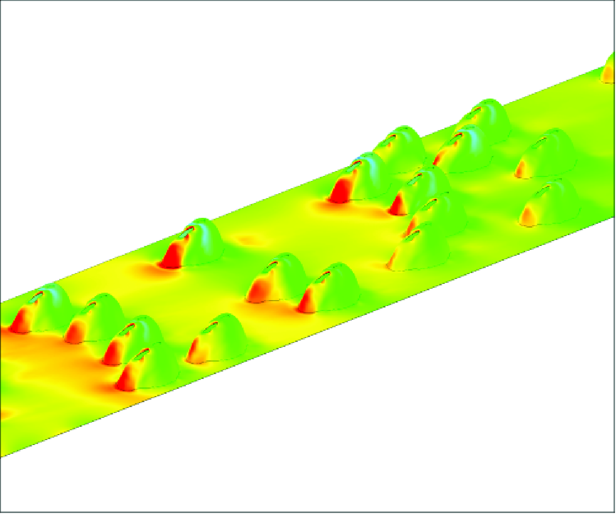
h) with respect to the velocity distribution in the corresponding fully developed open channel flow over a smooth bed. The interactions of the incoming flow with the protruding parts of the shells and with the excurrent-syphon jets generate large-scale turbulence and shedding behind the shells which amplifies the turbulent kinetic energy away from the channel bed. This is why, for sufficiently high
$=$
h) with respect to the velocity distribution in the corresponding fully developed open channel flow over a smooth bed. The interactions of the incoming flow with the protruding parts of the shells and with the excurrent-syphon jets generate large-scale turbulence and shedding behind the shells which amplifies the turbulent kinetic energy away from the channel bed. This is why, for sufficiently high
 $\rho$
N
, the maximum turbulent kinetic energy is not recorded in the immediate vicinity of the bed surface, as occurs in the corresponding case of fully developed flow over a smooth bed, but rather close to z
$\rho$
N
, the maximum turbulent kinetic energy is not recorded in the immediate vicinity of the bed surface, as occurs in the corresponding case of fully developed flow over a smooth bed, but rather close to z
 $=$
h (see double averaged profiles in figure 3
c).
$=$
h (see double averaged profiles in figure 3
c).

Figure 2. General features of the mean flow fields in the numerical solutions with
 $\rho$
N
$\rho$
N
 $=$
100 mussels m−2 and h/d
$=$
100 mussels m−2 and h/d
 $=$
0.5 case: (a) general view showing overall streamwise decay of the mean pressure Pmean
/(
$=$
0.5 case: (a) general view showing overall streamwise decay of the mean pressure Pmean
/(
 $\rho$
U0
2) over the channel bed due to the added drag by the mussels (VR
$\rho$
U0
2) over the channel bed due to the added drag by the mussels (VR
 $=$
0.13); (b) detail view showing mean pressure distributions on the protruding parts of the partially burrowed mussels situated near the leading edge of the mussel bed (VR
$=$
0.13); (b) detail view showing mean pressure distributions on the protruding parts of the partially burrowed mussels situated near the leading edge of the mussel bed (VR
 $=$
0.13); (c) detail view showing the mean scalar concentration, C/C0
, in a vertical-streamwise plane (y/d
$=$
0.13); (c) detail view showing the mean scalar concentration, C/C0
, in a vertical-streamwise plane (y/d
 $=$
3.3) cutting through several mussels (VR
$=$
3.3) cutting through several mussels (VR
 $=$
0.7) and 2-D streamlines visualising the curving of the excurrent-syphon jet; (d) detail view showing the mean spanwise vorticity,
$=$
0.7) and 2-D streamlines visualising the curving of the excurrent-syphon jet; (d) detail view showing the mean spanwise vorticity,
 $\omega$
yd/U0
, in a vertical-streamwise plane (y/d
$\omega$
yd/U0
, in a vertical-streamwise plane (y/d
 $=$
3.3) cutting through several mussels (VR
$=$
3.3) cutting through several mussels (VR
 $=$
0.7) and 2-D streamlines.
$=$
0.7) and 2-D streamlines.

Figure 3. Spatial evolution of the streamwise velocity, scalar concentration and turbulent kinetic energy inside the 2-D boundary layer in the
 $\rho$
N
$\rho$
N
 $=$
100 mussel m−2, VR
$=$
100 mussel m−2, VR
 $=$
0.13, h/d
$=$
0.13, h/d
 $=$
0.5 case: (a) vertical profiles of streamwise velocity, Uxz
/U0
; (b) vertical profiles of scalar concentration, Cxz
/C0
for Sc
$=$
0.5 case: (a) vertical profiles of streamwise velocity, Uxz
/U0
; (b) vertical profiles of scalar concentration, Cxz
/C0
for Sc
 $=$
1; (c) vertical profiles of turbulent kinetic energy, Kxz
/U0
2. The vertical arrow denotes the leading edge of the mussel bed (x/h
$=$
1; (c) vertical profiles of turbulent kinetic energy, Kxz
/U0
2. The vertical arrow denotes the leading edge of the mussel bed (x/h
 $=$
0). The horizontal dashed lines show the locations where z
$=$
0). The horizontal dashed lines show the locations where z
 $= \delta(x)$
. Panel (d) shows the effect of Schmidt number on the Cxz
/C0
profiles at x/h
$= \delta(x)$
. Panel (d) shows the effect of Schmidt number on the Cxz
/C0
profiles at x/h
 $=$
90, 130 and 190 based on simulations conducted with Sc
$=$
90, 130 and 190 based on simulations conducted with Sc
 $=$
1 and Sc
$=$
1 and Sc
 $=$
1000. Panel (e) compares the non-dimensional concentration profiles at x/h
$=$
1000. Panel (e) compares the non-dimensional concentration profiles at x/h
 $=$
100 and x/h
$=$
100 and x/h
 $=$
130 for Sc
$=$
130 for Sc
 $=$
1. The profiles are calculated using the inverse concentration approach and using the physical boundary conditions where the phytoplankton concentration of the incoming flow in the open channel is C’
$=$
1. The profiles are calculated using the inverse concentration approach and using the physical boundary conditions where the phytoplankton concentration of the incoming flow in the open channel is C’
 $=$
C0
and the concentration of the fluid entering the channel through the excurrent syphon is Ce’
$=$
C0
and the concentration of the fluid entering the channel through the excurrent syphon is Ce’
 $=$
0 (filtration rate, F
$=$
0 (filtration rate, F
 $=$
100 %). Results are also included for a simulation where mussels filter only 80 % of the amount of phytoplankton entering each mussel through the incurrent syphon (F
$=$
100 %). Results are also included for a simulation where mussels filter only 80 % of the amount of phytoplankton entering each mussel through the incurrent syphon (F
 $=$
80 %).
$=$
80 %).
Figure 2(c) shows the distribution of the time-averaged scalar concentration in a vertical-streamwise plane cutting through the excurrent syphons of two of the mussels in the array. They show how the jets of filtered water mix with the surrounding fluid. Most of the dilution occurs within 2–3h downstream of the incurrent syphon. The region shown in figure 2(c) is situated in the downstream part of the array where the concentration boundary layer already reached the top boundary. The mean concentration increases monotonically with the distance from the top boundary within most of the inertial layer except for the region of high concentration associated with the excurrent-syphon jets. The mean spanwise vorticity contours in figure 2(d) show that even for the highest filtering discharge (e.g. for VR
 $=$
0.7), the vertical penetration of the excurrent jet is less than 0.3d before the jet becomes more or less aligned with the streamwise direction. This is followed by a regime where the centreline of the diluted jet moves slightly away from the bottom surface as it is advected downstream.
$=$
0.7), the vertical penetration of the excurrent jet is less than 0.3d before the jet becomes more or less aligned with the streamwise direction. This is followed by a regime where the centreline of the diluted jet moves slightly away from the bottom surface as it is advected downstream.
Given the strong three-dimensional characteristics of the flow around the protruding shells, these effects are more easily studied and quantified using double-averaging, which is a technique widely employed to study flow past rough surfaces, including flow past large-scale bed roughness elements and flow over porous layers (e.g. see Nikora et al. Reference Nikora, McEwan, McLean, Coleman, Pokrajac and Walters2007; Coleman et al. Reference Coleman, Nikora, McLean and Schlicke2007). The averaging is performed along the spanwise direction in addition to averaging over time the instantaneous flow variables. The following formula is used to compute the width-averaged, mean streamwise velocity, Uxz :
 \begin{equation}U_{xz}(x,z)=\frac{1}{B'}\int _{0}^{B'}U(x,y,z){\rm d}y=\lt {U}\gt,\end{equation}
where B’(x,z) is the total width of the region occupied by the fluid (e.g. the interior of the protruding part of each shell is excluded). For z
 $\gt$
h, B’(x,z)
$\gt$
h, B’(x,z)
 $=$
B and (3.1) reduces to calculating the standard width-averaged value of the time-averaged 3-D velocity U(x,y,z). The
$=$
B and (3.1) reduces to calculating the standard width-averaged value of the time-averaged 3-D velocity U(x,y,z). The
 $\lt$
$\lt$
 $\gt$
operator denotes width-averaging of a time-averaged variable. A similar procedure is used to calculate the width-averaged mean scalar concentration, Cxz
, the width-averaged turbulent kinetic energy, Kxz
, and the width-averaged turbulent and dispersive stresses. Before discussing the profiles of Uxz
, Cxz
and Kxz
, we compared the double-averaged profiles of the velocity, concentration and TKE obtained using the 3-D mean flow fields over the full domain width and over half of the domain width for the
$\gt$
operator denotes width-averaging of a time-averaged variable. A similar procedure is used to calculate the width-averaged mean scalar concentration, Cxz
, the width-averaged turbulent kinetic energy, Kxz
, and the width-averaged turbulent and dispersive stresses. Before discussing the profiles of Uxz
, Cxz
and Kxz
, we compared the double-averaged profiles of the velocity, concentration and TKE obtained using the 3-D mean flow fields over the full domain width and over half of the domain width for the
 $\rho$
N
$\rho$
N
 $=$
100 mussel m−2, VR
$=$
100 mussel m−2, VR
 $=$
0.13, h/d
$=$
0.13, h/d
 $=$
0.5 case. The two sets of double-averaged profiles were found to be very close, which means that the domain width was large enough such that the characteristics of the double-averaged rough-bed boundary layer are basically independent of the domain width.
$=$
0.5 case. The two sets of double-averaged profiles were found to be very close, which means that the domain width was large enough such that the characteristics of the double-averaged rough-bed boundary layer are basically independent of the domain width.
The vertical profiles of Uxz
, Cxz
and Kxz
are shown in figures 3(a)–3(c) for the
 $\rho$
N
$\rho$
N
 $=$
100 mussel m−2, VR
$=$
100 mussel m−2, VR
 $=$
0.13, h/d
$=$
0.13, h/d
 $=$
0.5 case. The shape of the velocity profile changes quickly as the incoming (smooth-bed) fully developed flow (e.g. see profile at x/h
$=$
0.5 case. The shape of the velocity profile changes quickly as the incoming (smooth-bed) fully developed flow (e.g. see profile at x/h
 $=$
-10 in figure 3
a) moves over the region (x/h
$=$
-10 in figure 3
a) moves over the region (x/h
 $\gt$
0) containing mussels. A sudden decrease in the rate of increase of the streamwise velocity is observed in the velocity profiles between x/h
$\gt$
0) containing mussels. A sudden decrease in the rate of increase of the streamwise velocity is observed in the velocity profiles between x/h
 $=$
0 and x/h
$=$
0 and x/h
 $=$
120. As will be discussed later, the vertical location at which the sudden decrease starts corresponds to the top of the rough-bed boundary layer. The peak value of the scalar concentration profiles over the mussel bed is observed around the vertical location of the excurrent syphons (z/h ≈ 1, figure 3
b). Above this location, Cxz
decays monotonically towards zero, a value reached at the top of the concentration boundary layer. Past the location of the leading edge of the mussel bed, the vertical profiles and mean levels of the turbulent kinetic energy (figure 3
c) are very different from that in the incoming flow. A sharp amplification of more than five times with respect to the peak values in the approaching flow is observed for Kxz
starting a short distance downstream of the leading edge of the mussel bed (e.g. compare profile at x/h
$=$
120. As will be discussed later, the vertical location at which the sudden decrease starts corresponds to the top of the rough-bed boundary layer. The peak value of the scalar concentration profiles over the mussel bed is observed around the vertical location of the excurrent syphons (z/h ≈ 1, figure 3
b). Above this location, Cxz
decays monotonically towards zero, a value reached at the top of the concentration boundary layer. Past the location of the leading edge of the mussel bed, the vertical profiles and mean levels of the turbulent kinetic energy (figure 3
c) are very different from that in the incoming flow. A sharp amplification of more than five times with respect to the peak values in the approaching flow is observed for Kxz
starting a short distance downstream of the leading edge of the mussel bed (e.g. compare profile at x/h
 $=$
-10 with profiles at x/h
$=$
-10 with profiles at x/h
 $\gt$
10 in figure 3
c). These large values are induced by the eddies (e.g. vortex tubes) shed in the separated shear layers generated by the mussels situated close to the leading edge of the mussel bed. The region of high Kxz
occupies the entire roughness layer (0 ≤ z ≤ h) and its height over the top of the mussels increases monotonically in the streamwise direction. The Kxz
profiles in figure 3(c) suggest that the rough-bed boundary layer reaches the free surface before the trailing edge of the mussel bed (x/h
$\gt$
10 in figure 3
c). These large values are induced by the eddies (e.g. vortex tubes) shed in the separated shear layers generated by the mussels situated close to the leading edge of the mussel bed. The region of high Kxz
occupies the entire roughness layer (0 ≤ z ≤ h) and its height over the top of the mussels increases monotonically in the streamwise direction. The Kxz
profiles in figure 3(c) suggest that the rough-bed boundary layer reaches the free surface before the trailing edge of the mussel bed (x/h
 $=$
200). Non-zero values of the scalar concentration at the free surface are also observed for Cxz
starting around x/h
$=$
200). Non-zero values of the scalar concentration at the free surface are also observed for Cxz
starting around x/h
 $=$
120 (figure 3
b). Given that the incoming flow contains no scalar, the rough-bed boundary layer reaches the free surface before the end of the mussel bed.
$=$
120 (figure 3
b). Given that the incoming flow contains no scalar, the rough-bed boundary layer reaches the free surface before the end of the mussel bed.
Figure 3(d) investigates the Schmidt number effect on the concentration boundary layer for a mussel bed with
 $\rho$
N
$\rho$
N
 $=$
100 mussel m−2, VR
$=$
100 mussel m−2, VR
 $=$
0.13 and h/d
$=$
0.13 and h/d
 $=$
0.5 by comparing the double-averaged concentration profiles obtained from two simulations conducted with Sc
$=$
0.5 by comparing the double-averaged concentration profiles obtained from two simulations conducted with Sc
 $=$
1 and Sc
$=$
1 and Sc
 $=$
1000. As the dynamics of the phytoplankton concentration is simulated using a passive scalar equation, the velocity fields and the double-averaged profiles of the velocity and turbulent kinetic energy are not affected by the value of the Schmidt number. The same is true for the thickness of the boundary layer based on the vertical profiles of Kxz
. As opposed to a concentration boundary layer developing over a smooth bed, where the value of the Schmidt number can significantly affect the growth rate of the boundary layer, results in figure 3(d) show this is not the case for the boundary layer developing over the mussel bed. In particular, the effect of increasing the Schmidt number from 1 to 1000 is negligible inside the inertial layer, so
$=$
1000. As the dynamics of the phytoplankton concentration is simulated using a passive scalar equation, the velocity fields and the double-averaged profiles of the velocity and turbulent kinetic energy are not affected by the value of the Schmidt number. The same is true for the thickness of the boundary layer based on the vertical profiles of Kxz
. As opposed to a concentration boundary layer developing over a smooth bed, where the value of the Schmidt number can significantly affect the growth rate of the boundary layer, results in figure 3(d) show this is not the case for the boundary layer developing over the mussel bed. In particular, the effect of increasing the Schmidt number from 1 to 1000 is negligible inside the inertial layer, so
 $\delta$
C
is basically independent of the Schmidt number over this interval. Some mild Schmidt number effects are present inside the inner layer. The main reason is that mixing between the filtered water and the phytoplankton-rich water is driven, to a large extent, by the larger-scale turbulent eddies generated by the emerged parts of the mussel shells (e.g. see Wu et al. Reference Wu, Constantinescu and Zeng2020 for a detailed discussion of the coherent structures generated by individual partially burrowed mussels). The main eddies are the vortex tubes generated in the separated shear layers and large-scale hairpins that scale with the height of the protruding part of the mussels. The size and dynamics of these eddies are independent of the value of the Schmidt number. This is the main reason why analysis performed based on simulations conducted with Sc
$\delta$
C
is basically independent of the Schmidt number over this interval. Some mild Schmidt number effects are present inside the inner layer. The main reason is that mixing between the filtered water and the phytoplankton-rich water is driven, to a large extent, by the larger-scale turbulent eddies generated by the emerged parts of the mussel shells (e.g. see Wu et al. Reference Wu, Constantinescu and Zeng2020 for a detailed discussion of the coherent structures generated by individual partially burrowed mussels). The main eddies are the vortex tubes generated in the separated shear layers and large-scale hairpins that scale with the height of the protruding part of the mussels. The size and dynamics of these eddies are independent of the value of the Schmidt number. This is the main reason why analysis performed based on simulations conducted with Sc
 $=$
1 is also fairly representative of a much larger range of Schmidt numbers for the concentration boundary layer generated by the partially burrowed mussels.
$=$
1 is also fairly representative of a much larger range of Schmidt numbers for the concentration boundary layer generated by the partially burrowed mussels.
Given that the velocity fields are not affected by the use of the inverse concentration approach and that the relationship between the phytoplankton concentration, C’, and the concentration C used in the inverse concentration approach is linear (i.e. C
 $=$
C0
- C’), the predicted distributions of C’ and C’xz
(or, equivalently, of C
0
- C’ and C
0
- C’xz
) should be fully equivalent to those obtained using the inverse concentration approach. This is confirmed by results of two simulations (Sc
$=$
C0
- C’), the predicted distributions of C’ and C’xz
(or, equivalently, of C
0
- C’ and C
0
- C’xz
) should be fully equivalent to those obtained using the inverse concentration approach. This is confirmed by results of two simulations (Sc
 $=$
1, F
$=$
1, F
 $=$
100 %) of the
$=$
100 %) of the
 $\rho$
N
$\rho$
N
 $=$
100 mussel m−2, VR
$=$
100 mussel m−2, VR
 $=$
0.13, h/d
$=$
0.13, h/d
 $=$
0.5 case conducted with and without the inverse concentration approach. For example, figure 3(e) shows that the profiles of 1 - C’xz
/C0
and Cxz
/C0
from two simulations in which the scalar transport equation is solved for C’ and respectively for C are identical at x/h
$=$
0.5 case conducted with and without the inverse concentration approach. For example, figure 3(e) shows that the profiles of 1 - C’xz
/C0
and Cxz
/C0
from two simulations in which the scalar transport equation is solved for C’ and respectively for C are identical at x/h
 $=$
100 and x/h
$=$
100 and x/h
 $=$
130.
$=$
130.
Even though in most models it is generally assumed that mussels filter all the phytoplankton entering through their incurrent syphon (F
 $=$
100 %), it is possible that not all plankton is filtered by these organisms (F
$=$
100 %), it is possible that not all plankton is filtered by these organisms (F
 $\lt$
100 %). Figure 3(e) compares the profiles of Cxz
/C0
from two simulations of the
$\lt$
100 %). Figure 3(e) compares the profiles of Cxz
/C0
from two simulations of the
 $\rho$
N
$\rho$
N
 $=$
100 mussel m−2, VR
$=$
100 mussel m−2, VR
 $=$
0.13, h/d
$=$
0.13, h/d
 $=$
0.5 case performed with F
$=$
0.5 case performed with F
 $=$
100 % and F
$=$
100 % and F
 $=$
80 %. As expected, the values of Cxz
/C0
predicted in the F
$=$
80 %. As expected, the values of Cxz
/C0
predicted in the F
 $=$
80 % simulation are smaller. However, if the profiles in the F
$=$
80 % simulation are smaller. However, if the profiles in the F
 $=$
80 % simulation are rescaled using the maximum concentration, which is very close to the excurrent syphon concentration, the profiles in the F
$=$
80 % simulation are rescaled using the maximum concentration, which is very close to the excurrent syphon concentration, the profiles in the F
 $=$
80 % simulation become close to identical to those predicted in the F
$=$
80 % simulation become close to identical to those predicted in the F
 $=$
100 % simulation. This shows that results from the present study can also be used to make predictions for cases where the mussel filtration rate is less than 100 %.
$=$
100 % simulation. This shows that results from the present study can also be used to make predictions for cases where the mussel filtration rate is less than 100 %.
Figure 4 compares the streamwise distributions of the peak values of the vertical profiles of Cxz
and Kxz
in the simulations performed with Sc
 $=$
1 and F
$=$
1 and F
 $=$
100 %. These peak values are denoted Cmax
and Kmax
, respectively. While the streamwise growth of Cmax
is a direct consequence of the increase in the number of jets entering the domain with increasing x/h, the streamwise increase of Kmax
is because energetic coherent structures passing through a certain cross-section are generated by all the mussels situated in between the leading edge of the mussel bed and that section. For constant VR and h/d, Cmax
and Kmax
increase monotonically with
$=$
100 %. These peak values are denoted Cmax
and Kmax
, respectively. While the streamwise growth of Cmax
is a direct consequence of the increase in the number of jets entering the domain with increasing x/h, the streamwise increase of Kmax
is because energetic coherent structures passing through a certain cross-section are generated by all the mussels situated in between the leading edge of the mussel bed and that section. For constant VR and h/d, Cmax
and Kmax
increase monotonically with
 $\rho$
N
, which is expected given that the bed contains more mussels per unit streamwise length (figure 4
a). Moreover, the average streamwise rate of growth of Cmax
also increases with
$\rho$
N
, which is expected given that the bed contains more mussels per unit streamwise length (figure 4
a). Moreover, the average streamwise rate of growth of Cmax
also increases with
 $\rho$
N. Given that most of the large-scale coherent structures generated by mussels scale with the height of their protruding part, it is not surprising to see a decrease of 30 %–45 % for Kmax
as h/d decreases from 0.5 to 0.3 in the simulations with
$\rho$
N. Given that most of the large-scale coherent structures generated by mussels scale with the height of their protruding part, it is not surprising to see a decrease of 30 %–45 % for Kmax
as h/d decreases from 0.5 to 0.3 in the simulations with
 $\rho$
N
$\rho$
N
 $=$
100 mussels m−2 and VR
$=$
100 mussels m−2 and VR
 $=$
0.13 (figure 4
b). However, the effect of decreasing h/d on Cmax
is negligible. For constant
$=$
0.13 (figure 4
b). However, the effect of decreasing h/d on Cmax
is negligible. For constant
 $\rho$
N
and h/d, Kmax
increases with increasing the filtering discharge due to the increased momentum of the excurrent jets (figure 4
c). The rate of increase of Kmax
with VR decreases above medium values (e.g. VR ≥ 0.13) of the filtering discharge.
$\rho$
N
and h/d, Kmax
increases with increasing the filtering discharge due to the increased momentum of the excurrent jets (figure 4
c). The rate of increase of Kmax
with VR decreases above medium values (e.g. VR ≥ 0.13) of the filtering discharge.

Figure 4. Streamwise variation of the peak scalar concentration and turbulent kinetic energy inside the rough-bed turbulent boundary layer: (a) Cmax
/C0
and Kmax
/U0
2 versus
 $\rho$
N
for VR
$\rho$
N
for VR
 $=$
0.13, h/d
$=$
0.13, h/d
 $=$
0.5; (b) Cmax
/C0
and Kmax
/U0
2 versus h/d for
$=$
0.5; (b) Cmax
/C0
and Kmax
/U0
2 versus h/d for
 $\rho$
N
$\rho$
N
 $=$
100 mussels m−2, VR
$=$
100 mussels m−2, VR
 $=$
0.13; (c) Kmax
/U0
2 versus VR for
$=$
0.13; (c) Kmax
/U0
2 versus VR for
 $\rho$
N
$\rho$
N
 $=$
100 mussels m−2, h/d
$=$
100 mussels m−2, h/d
 $=$
0.5.
$=$
0.5.
The vertical positions corresponding to the peak values in the vertical profiles of Cxz
and Kxz
are denoted zC
and zK
, respectively. Their non-dimensional values, zC
/d and zK
/d are varying very little in between the leading edge of the mussel bed and its trailing edge. Both variables are practically independent of the mussel array density. Figure 5 shows that increasing the filtering rate results in larger values of zC
/d and zK
/d. As the discharge of the vertically oriented excurrent jet increases, so does the elevation where the jet aligns with the streamwise direction (see also figure 2
c). Increasing the height of the protruding parts of the mussels results in an increase of both zC
/d and zK
/d. For example, as h/d increases from 0.3 to 0.5, zC
/d increases from 0.35 to 0.55, and zK
/h from 0.38 to 0.57 in the VR
 $=$
0.13 simulations.
$=$
0.13 simulations.

Figure 5. Mean vertical elevations, zC
/d and zK
/d, where the peak values in the scalar concentration profile and in the turbulent kinetic energy profile are recorded. Results are basically independent of
 $\rho$
N
.
$\rho$
N
.
3.2. Boundary layer thickness
The incoming flow upstream of the mussel bed is fully developed. This makes it difficult to identify the edge of the rough-bed boundary layer based on analysing the momentum. Given also that a main goal of the present study is to describe the concentration boundary layer associated with phytoplankton removal by the mussels, the definition used to identify the extremity of the rough-bed boundary layer is based on the distribution of Cxz
. At each streamwise location, the thickness of the concentration boundary layer,
 $\delta$
C
, is defined as the vertical location where Cxz
becomes less than 1% of the maximum value recorded at z
$\delta$
C
, is defined as the vertical location where Cxz
becomes less than 1% of the maximum value recorded at z
 $=$
zC
(figure 6
b), i.e. Cxz
(z
$=$
zC
(figure 6
b), i.e. Cxz
(z
 $=$
$=$
 $\delta$
C
)
$\delta$
C
)
 $=$
0.01Cmax
. The thickness of the momentum boundary layer,
$=$
0.01Cmax
. The thickness of the momentum boundary layer,
 $\delta$
, is assumed equal to
$\delta$
, is assumed equal to
 $\delta$
C
. O’Riordan et al., (Reference O’Riordan, Monismith and Koseff1995) observed a strong connection between
$\delta$
C
. O’Riordan et al., (Reference O’Riordan, Monismith and Koseff1995) observed a strong connection between
 $\delta$
C
and
$\delta$
C
and
 $\delta$
in their experiments conducted with a bed of active-filtering clams.
$\delta$
in their experiments conducted with a bed of active-filtering clams.

Figure 6. Sketch showing vertical profiles of the width-averaged mean streamwise velocity, mean scalar concentration and turbulent kinetic energy in between the bed (z
 $=$
0) and the top of the rough-bed turbulent boundary layer: (a) Uxz
; (b) Cxz
; (c) Kxz
. The inertial layer is situated in between the top of the mussels (z
$=$
0) and the top of the rough-bed turbulent boundary layer: (a) Uxz
; (b) Cxz
; (c) Kxz
. The inertial layer is situated in between the top of the mussels (z
 $=$
h) and the top edge of the boundary layer. The roughness layer (0
$=$
h) and the top edge of the boundary layer. The roughness layer (0
 $\lt$
z
$\lt$
z
 $\lt$
h) contains a linear sublayer (0
$\lt$
h) contains a linear sublayer (0
 $\lt$
z
$\lt$
z
 $\lt$
$\lt$
 $\delta$
m
) close to the bed and an exponential sublayer (
$\delta$
m
) close to the bed and an exponential sublayer (
 $\delta$
m
$\delta$
m
 $\lt$
z
$\lt$
z
 $\lt$
h), where Uxz
decays exponentially with the distance from the top of the roughness layer. The turbulent boundary layer width is denoted
$\lt$
h), where Uxz
decays exponentially with the distance from the top of the roughness layer. The turbulent boundary layer width is denoted
 $\delta$
,
$\delta$
,
 $\delta$
C
and
$\delta$
C
and
 $\delta$
K
in the three frames. Also shown are the locations z
$\delta$
K
in the three frames. Also shown are the locations z
 $=$
zC
and z
$=$
zC
and z
 $=$
zK
, where Cxz
$=$
zK
, where Cxz
 $=$
Cmax
and Kxz
$=$
Cmax
and Kxz
 $=$
Kmax
. The Cxz
and Kxz
profiles are self-similar for zC
$=$
Kmax
. The Cxz
and Kxz
profiles are self-similar for zC
 $\lt$
z
$\lt$
z
 $\lt$
$\lt$
 $\delta$
C
and zK
$\delta$
C
and zK
 $\lt$
z
$\lt$
z
 $\lt$
$\lt$
 $\delta$
K
, where zc
and zk
are only slightly larger than h.
$\delta$
K
, where zc
and zk
are only slightly larger than h.
Once
 $\delta$
C
is calculated, one can try scaling the normalised concentration profiles of Cxz
/Cmax
at different streamwise locations to investigate an eventual self-similarity of the mean concentration profiles for zC
$\delta$
C
is calculated, one can try scaling the normalised concentration profiles of Cxz
/Cmax
at different streamwise locations to investigate an eventual self-similarity of the mean concentration profiles for zC
 $\lt$
z
$\lt$
z
 $\lt$
$\lt$
 $\delta$
C
. The scalar concentration profiles are plotted as a function of the non-dimensional vertical distance, z’
$\delta$
C
. The scalar concentration profiles are plotted as a function of the non-dimensional vertical distance, z’
 $=$
(z-zC
)/(
$=$
(z-zC
)/(
 $\delta$
C
-zC
). Figure 7 shows the scaled profiles for the
$\delta$
C
-zC
). Figure 7 shows the scaled profiles for the
 $\rho$
N
$\rho$
N
 $=$
100 mussel m−2, VR
$=$
100 mussel m−2, VR
 $=$
0.13, h/d
$=$
0.13, h/d
 $=$
0.5 case between x/h
$=$
0.5 case between x/h
 $=$
40 and the location where the concentration boundary layer reaches the free surface (x/h
$=$
40 and the location where the concentration boundary layer reaches the free surface (x/h
 $=$
120). Though the scaled profiles do not collapse into a unique curve, the differences are small especially if one considers the finite width of the channel, the irregular distribution of the mussels and the presence of clusters of mussels in some regions. So, one can conclude that, in a good approximation, self-similarity is achieved some distance from the leading edge of the mussel bed. The aforementioned procedure to determine
$=$
120). Though the scaled profiles do not collapse into a unique curve, the differences are small especially if one considers the finite width of the channel, the irregular distribution of the mussels and the presence of clusters of mussels in some regions. So, one can conclude that, in a good approximation, self-similarity is achieved some distance from the leading edge of the mussel bed. The aforementioned procedure to determine
 $\delta$
C
cannot be used once the boundary layer reaches the free surface. However, an appropriate value for
$\delta$
C
cannot be used once the boundary layer reaches the free surface. However, an appropriate value for
 $\delta$
C
can be estimated at locations situated between x/h
$\delta$
C
can be estimated at locations situated between x/h
 $=$
120 and the trailing edge of the mussel bed assuming the scaled concentration profiles should continue to be close to those predicted at streamwise locations where
$=$
120 and the trailing edge of the mussel bed assuming the scaled concentration profiles should continue to be close to those predicted at streamwise locations where
 $\delta$
C
$\delta$
C
 $\lt$
D. These profiles are also plotted in figure 7 in between z
$\lt$
D. These profiles are also plotted in figure 7 in between z
 $=$
zC
and z
$=$
zC
and z
 $=$
D. Self-similarity for the scalar concentration profiles is not well satisfied for x/h ≤ 40. Rough-bed boundary layers developing over sparse roughness elements are expected to require an initial distance before they achieve self-similarity.
$=$
D. Self-similarity for the scalar concentration profiles is not well satisfied for x/h ≤ 40. Rough-bed boundary layers developing over sparse roughness elements are expected to require an initial distance before they achieve self-similarity.

Figure 7. Normalised profiles of Cxz
for z
 $\gt$
zC
at streamwise locations where the boundary layer is situated beneath the free surface (x/h ≤ 120) and at downstream locations (x/h
$\gt$
zC
at streamwise locations where the boundary layer is situated beneath the free surface (x/h ≤ 120) and at downstream locations (x/h
 $\gt$
120) in the
$\gt$
120) in the
 $\rho$
N
$\rho$
N
 $=$
100 mussel m−2, VR
$=$
100 mussel m−2, VR
 $=$
0.13, h/d
$=$
0.13, h/d
 $=$
0.5 case. For x/h
$=$
0.5 case. For x/h
 $\gt$
120, the profiles extend only from z
$\gt$
120, the profiles extend only from z
 $=$
0 to z
$=$
0 to z
 $=$
D. The red dashed lines show the location where z
$=$
D. The red dashed lines show the location where z
 $=$
D. The black dashed line shows the self-similar profile for the case.
$=$
D. The black dashed line shows the self-similar profile for the case.
A similar approach to that used to define
 $\delta$
C
can be used to determine the thickness of the rough-bed boundary layer based on the vertical profiles of Kxz
(figure 6
c). This thickness, denoted
$\delta$
C
can be used to determine the thickness of the rough-bed boundary layer based on the vertical profiles of Kxz
(figure 6
c). This thickness, denoted
 $\delta$
K
, is defined as the vertical location where Kxz
$\delta$
K
, is defined as the vertical location where Kxz
 $=$
0.01Kmax
. The same procedure used in figure 7 to scale the concentration profiles for zC
$=$
0.01Kmax
. The same procedure used in figure 7 to scale the concentration profiles for zC
 $\lt$
z
$\lt$
z
 $\lt$
$\lt$
 $\delta$
C
is used for the turbulent kinetic energy profiles but with
$\delta$
C
is used for the turbulent kinetic energy profiles but with
 $\delta$
C
replaced by
$\delta$
C
replaced by
 $\delta$
K
and zC
replaced by zK
in the definition of the normalised vertical distance. Downstream of the location where the boundary layer reaches the free surface, one can determine an approximate value for
$\delta$
K
and zC
replaced by zK
in the definition of the normalised vertical distance. Downstream of the location where the boundary layer reaches the free surface, one can determine an approximate value for
 $\delta$
K
such that the scaled profile of Kxz
in between z
$\delta$
K
such that the scaled profile of Kxz
in between z
 $=$
zK
and z
$=$
zK
and z
 $=$
D is the closest possible to the self-similar profile determined in between the upstream location where the profiles become approximately self-similar and the location where the boundary layer reaches the free surface.
$=$
D is the closest possible to the self-similar profile determined in between the upstream location where the profiles become approximately self-similar and the location where the boundary layer reaches the free surface.
For all cases, the streamwise variation of
 $\delta$
C
is quite close to that of
$\delta$
C
is quite close to that of
 $\delta$
K
(figures 8
a and 8
b). The difference between
$\delta$
K
(figures 8
a and 8
b). The difference between
 $\delta$
C
and
$\delta$
C
and
 $\delta$
K
at any given streamwise location is of the order of 0.2–0.6h. For constant VR and h/d, the rough-bed boundary layer thickness increases with the mussel array density (figure 8
a). For the range of
$\delta$
K
at any given streamwise location is of the order of 0.2–0.6h. For constant VR and h/d, the rough-bed boundary layer thickness increases with the mussel array density (figure 8
a). For the range of
 $\rho$
N
values considered in the present study, the mean flow three dimensionality and the turbulent kinetic energy levels inside the boundary layer grow with increasing number of roughness elements per unit surface. As a result, the probability of having energetic eddies generated by the interaction of the flow with the individual roughness elements penetrating further away from the channel bed, as they are advected downstream, also increases with
$\rho$
N
values considered in the present study, the mean flow three dimensionality and the turbulent kinetic energy levels inside the boundary layer grow with increasing number of roughness elements per unit surface. As a result, the probability of having energetic eddies generated by the interaction of the flow with the individual roughness elements penetrating further away from the channel bed, as they are advected downstream, also increases with
 $\rho$
N
. For Rex
$\rho$
N
. For Rex
 $\gt$
300 000, the streamwise rates of growth of
$\gt$
300 000, the streamwise rates of growth of
 $\delta$
C
and
$\delta$
C
and
 $\delta$
K
decrease with increasing
$\delta$
K
decrease with increasing
 $\rho$
N
.
$\rho$
N
.

Figure 8. Variation of the rough-bed turbulent boundary layer thickness and momentum thickness with Rex
 $=$
xU0
/
$=$
xU0
/
 $\nu$
: (a)
$\nu$
: (a)
 $\delta$
C
/h (solid lines) and
$\delta$
C
/h (solid lines) and
 $\delta$
K
/h (dashed lines) versus
$\delta$
K
/h (dashed lines) versus
 $\rho$
N for VR
$\rho$
N for VR
 $=$
0.13, h/d
$=$
0.13, h/d
 $=$
0.5; (b)
$=$
0.5; (b)
 $\delta$
C
/h and
$\delta$
C
/h and
 $\delta$
K
/h versus h/d for
$\delta$
K
/h versus h/d for
 $\rho$
N
$\rho$
N
 $=$
100 mussels m−2, VR
$=$
100 mussels m−2, VR
 $=$
0.13; (c) θ/h versus
$=$
0.13; (c) θ/h versus
 $\rho$
N
for VR
$\rho$
N
for VR
 $=$
0.13, h/d
$=$
0.13, h/d
 $=$
0.5; (d) θ/h versus h/d for
$=$
0.5; (d) θ/h versus h/d for
 $\rho$
N
$\rho$
N
 $=$
100 mussels m−2, VR
$=$
100 mussels m−2, VR
 $=$
0.13. Panel (a) also shows
$=$
0.13. Panel (a) also shows
 $\delta$
K
/h for
$\delta$
K
/h for
 $\rho$
N
$\rho$
N
 $=$
55 mussels m−2, VR
$=$
55 mussels m−2, VR
 $=$
0.00, h/d
$=$
0.00, h/d
 $=$
0.5.
$=$
0.5.
For constant
 $\rho$
N
and h/d, the boundary layer thickness increases monotonically with VR, but the effect is very small. In particular, the streamwise variation of
$\rho$
N
and h/d, the boundary layer thickness increases monotonically with VR, but the effect is very small. In particular, the streamwise variation of
 $\delta$
K
in the simulations conducted with VR
$\delta$
K
in the simulations conducted with VR
 $=$
0 and VR
$=$
0 and VR
 $=$
0.13 is basically identical (see figure 8
a for
$=$
0.13 is basically identical (see figure 8
a for
 $\rho$
N
$\rho$
N
 $=$
25 mussels m−2). Though the excurrent-syphon jet is oriented vertically, increasing the vertical momentum of these jets does not result in a noticeable increase of their capacity to displace larger-scale eddies advected from upstream towards the free surface, at least for the cases investigated in this study conducted with VR ≤ 0.7.
$=$
25 mussels m−2). Though the excurrent-syphon jet is oriented vertically, increasing the vertical momentum of these jets does not result in a noticeable increase of their capacity to displace larger-scale eddies advected from upstream towards the free surface, at least for the cases investigated in this study conducted with VR ≤ 0.7.
Increasing h/d, while keeping
 $\rho$
N
and VR constant, results in higher values of
$\rho$
N
and VR constant, results in higher values of
 $\delta$
C
and
$\delta$
C
and
 $\delta$
K
at all streamwise locations (figure 8
b). The same is true for
$\delta$
K
at all streamwise locations (figure 8
b). The same is true for
 $\delta$
C
- zC
and
$\delta$
C
- zC
and
 $\delta$
K
- zK
. This happens because the degree of bluntness and the size of the roughness elements increase with increasing h. As a result, larger, more coherent eddies are generated by the interactions between the overflow and each individual roughness element in the cases with a larger h/d. However, when scaled with the height of the roughness elements, the normalised boundary layer thickness (
$\delta$
K
- zK
. This happens because the degree of bluntness and the size of the roughness elements increase with increasing h. As a result, larger, more coherent eddies are generated by the interactions between the overflow and each individual roughness element in the cases with a larger h/d. However, when scaled with the height of the roughness elements, the normalised boundary layer thickness (
 $\delta$
C
/h,
$\delta$
C
/h,
 $\delta$
K
/h) decreases with increasing h, as observed in figure 8(b). The streamwise rates of growth of
$\delta$
K
/h) decreases with increasing h, as observed in figure 8(b). The streamwise rates of growth of
 $\delta$
C
and
$\delta$
C
and
 $\delta$
K
in the simulations conducted with h/d
$\delta$
K
in the simulations conducted with h/d
 $=$
0.3 and 0.5 are close for Rex
$=$
0.3 and 0.5 are close for Rex
 $\gt$
300 000.
$\gt$
300 000.
The increase of the momentum thickness, θ, with the Reynolds number Rex
 $=$
xUo
/
$=$
xUo
/
 $\nu$
shows some interesting trends. For constant VR and h/d (figure 8
c), the rate of increase of θ becomes small for Rex
$\nu$
shows some interesting trends. For constant VR and h/d (figure 8
c), the rate of increase of θ becomes small for Rex
 $\gt$
130 000 in the simulation conducted with the smallest value of the mussel array density (
$\gt$
130 000 in the simulation conducted with the smallest value of the mussel array density (
 $\rho$
N
$\rho$
N
 $=$
10 mussels m−2) while the increase of θ with Rex
for Rex
$=$
10 mussels m−2) while the increase of θ with Rex
for Rex
 $\gt$
100 000 is close to linear until the end of the mussel bed in the simulation conducted with the highest value of the mussel array density (
$\gt$
100 000 is close to linear until the end of the mussel bed in the simulation conducted with the highest value of the mussel array density (
 $\rho$
N
$\rho$
N
 $=$
100 mussels m−2). For constant
$=$
100 mussels m−2). For constant
 $\rho$
N
and VR, the variation of the non-dimensional momentum thickness, θ/h, is basically independent of h (figure 8
d). Analysis of the data also showed that the value of VR has a negligible effect on the streamwise variation of θ.
$\rho$
N
and VR, the variation of the non-dimensional momentum thickness, θ/h, is basically independent of h (figure 8
d). Analysis of the data also showed that the value of VR has a negligible effect on the streamwise variation of θ.
4. Momentum boundary layer
4.1. Streamwise velocity
Analytical models were already proposed to approximate the profiles of the mean (time- and spatially averaged) streamwise velocity in boundary layers developing over other types of large-scale roughness elements (e.g. cubes and rectangular prisms, 2-D ribs, vertical cylinders) with no local mass exchange. In general, such models assume that the boundary layer is composed of a roughness/canopy layer (figure 6 a) extending up to the top of the roughness elements, or up to a distance equal to the mean plus the standard deviation of the elements’ height for cases with non-identical roughness elements, and of an inertial layer above it (e.g. Raupach, Antonia & Rajagopalan Reference Raupach, Antonia and Rajagopalan1991; Yang et al. Reference Yang, Sadique, Mittal and Meneveau2016). Cionco (Reference Cionco1965) was the first to propose an exponential variation of the mean streamwise velocity in between the top of the roughness layer and some distance from the channel bed. The exponential variation can be obtained by assuming an equilibrium between the vertical gradient of the momentum flux and the distributed drag from the roughness elements in the streamwise momentum equation and a constant mixing length eddy viscosity (Cionco Reference Cionco1965; Coceal & Belcher Reference Coceal and Belcher2004). A logarithmic variation is generally assumed inside the inertial layer with the roughness length assumed to be proportional to the height of the roughness elements (e.g. see Butman et al. Reference Butman, Frechette, Geyer and Starczak1994; Nikora et al. Reference Nikora, Green, Thrush, Hume and Goring2002; Van Duren et al. Reference Van Duren, Herman, Sandee and Heip2006). In particular, Yang et al. (Reference Yang, Sadique, Mittal and Meneveau2016) assumed a modified log-law variation of the mean streamwise velocity supplemented by a law-of-the-wake component.
Given that the present study considers a boundary layer developing over much more streamlined roughness elements and because of the presence of local mass exchange, one will start by investigating if the types of functions previously proposed to approximate the velocity profile over the roughness and inertial layers also apply for a boundary layer generated over a mussel bed with active filtering. We will also try to extend the analytical model such that it can be applied starting at the bed, where the velocity is zero. The analytical model of Cionco (Reference Cionco1965) cannot be applied close to the bed as it predicts a non-zero velocity at z
 $=$
0. Given that in the present simulations the viscous sublayer at the channel bed is resolved, the predicted near-bed velocity profiles should be accurate. Analysis of the streamwise velocity profiles shows that Uxz
increases linearly with z until a certain elevation situated way above the viscous sublayer generated on the horizontal bed surface in the 3-D simulations. The velocity then transitions rapidly to an exponential variation starting at z
$=$
0. Given that in the present simulations the viscous sublayer at the channel bed is resolved, the predicted near-bed velocity profiles should be accurate. Analysis of the streamwise velocity profiles shows that Uxz
increases linearly with z until a certain elevation situated way above the viscous sublayer generated on the horizontal bed surface in the 3-D simulations. The velocity then transitions rapidly to an exponential variation starting at z
 $=$
$=$
 $\delta$
m
. So, we propose to split the roughness layer into a linear sublayer that also contains the short transition region and an exponential sublayer (
$\delta$
m
. So, we propose to split the roughness layer into a linear sublayer that also contains the short transition region and an exponential sublayer (
 $\delta$
m
$\delta$
m
 $\lt$
z
$\lt$
z
 $\lt$
h), as shown in figure 6(a).
$\lt$
h), as shown in figure 6(a).
The velocity inside the linear sublayer is
 \begin{equation}U_{xz}=\frac{U_{m}z}{\delta _{m}},\end{equation}
where Um
is the velocity measured at the bottom of the exponential sublayer (z
 $=$
$=$
 $\delta$
m
).
$\delta$
m
).
The velocity profile inside the exponential sublayer is
 \begin{equation}U_{xz}=U_{h}e^{\frac{a(z-h)}{h}},\end{equation}
where U
h
is the mean streamwise velocity measured at the top of the mussel (z
 $=$
h) and a is an attenuation parameter for the exponential function. Yang et al. (Reference Yang, Sadique, Mittal and Meneveau2016) found that the attenuation parameter is correlated with the density and spatial distribution of the roughness elements.
$=$
h) and a is an attenuation parameter for the exponential function. Yang et al. (Reference Yang, Sadique, Mittal and Meneveau2016) found that the attenuation parameter is correlated with the density and spatial distribution of the roughness elements.
Following Yang et al. (Reference Yang, Sadique, Mittal and Meneveau2016), the assumed velocity profile inside the inertial layer (h
 $\lt$
z
$\lt$
z
 $\lt$
$\lt$
 $\delta$
) is
$\delta$
) is
 \begin{equation}U_{xz}=\frac{u_{\tau }}{\kappa }\mathit{\ln } \frac{z-d_{0}}{z_{0}}+\frac{\Pi u_{\tau }}{\kappa }w\left(\frac{z}{\delta }\right),\end{equation}
where
 $\kappa$
is the von Karman constant, z0
is the hydrodynamic roughness length,
$\kappa$
is the von Karman constant, z0
is the hydrodynamic roughness length,
 $u_{\tau }$
is the mean, width-averaged bed friction velocity at the bed and
$u_{\tau }$
is the mean, width-averaged bed friction velocity at the bed and
 $\Pi$
is the wake component coefficient. The expression for the law-of-the-wake function is
$\Pi$
is the wake component coefficient. The expression for the law-of-the-wake function is
 $w({z}/{\delta })=2\mathit{\sin }^{2} (({\pi }/{2})({z}/{\delta }))$
based on Coles (Reference Coles1956). The displacement height, d0
, is set equal to the centroid height of the distributed drag force (Jackson Reference Jackson1981), e.g. to the distance from the bed where the resultant drag force is applied on the mussel shell. This variable accounts for the fact that the roughness displaces the entire flow upwards (Raupach et al. Reference Raupach, Antonia and Rajagopalan1991). This is why, the origin of z in the standard log law for rough surfaces is modified by d0
in (4.3). For any mussel in the array, d0
can be calculated based on the mean pressure distribution on the mussel shell, Pmean
, as follows:
$w({z}/{\delta })=2\mathit{\sin }^{2} (({\pi }/{2})({z}/{\delta }))$
based on Coles (Reference Coles1956). The displacement height, d0
, is set equal to the centroid height of the distributed drag force (Jackson Reference Jackson1981), e.g. to the distance from the bed where the resultant drag force is applied on the mussel shell. This variable accounts for the fact that the roughness displaces the entire flow upwards (Raupach et al. Reference Raupach, Antonia and Rajagopalan1991). This is why, the origin of z in the standard log law for rough surfaces is modified by d0
in (4.3). For any mussel in the array, d0
can be calculated based on the mean pressure distribution on the mussel shell, Pmean
, as follows:
 \begin{equation}d_{0}=\frac{\int C_{{\rm d}x}^{mean}(U^{mean})^{2}z{\rm d}A}{\int C_{{\rm d}x}^{mean}(U^{mean})^{2}{\rm d}A}=\frac{\int P^{mean}n_{x}z{\rm d}A}{\int P^{mean}n_{x}{\rm d}A},\end{equation}
where nx
is the x component of the outward unit vector and dA is the area element, P is the pressure, C
dx
is the streamwise drag coefficient and the superscript ‘mean’ indicates time-averaged values. The integration is carried out over the protruding part of the mussel shell. To obtain the values of u
 $_\tau$
and z0
in (4.3), one needs to use the predicted velocity profile. Applying the boundary conditions at the bottom (Uxz
(h)
$_\tau$
and z0
in (4.3), one needs to use the predicted velocity profile. Applying the boundary conditions at the bottom (Uxz
(h)
 $=$
Uh
) and top (Uxz
(
$=$
Uh
) and top (Uxz
(
 $\delta$
)
$\delta$
)
 $=$
U
$=$
U
 $_{\delta}$
) of the inertial layer, one obtains two equations that can be solved to determine u
$_{\delta}$
) of the inertial layer, one obtains two equations that can be solved to determine u
 $_\tau$
and z0
:
$_\tau$
and z0
:
 \begin{equation}U_{h}=\frac{u_{\tau }}{\kappa }\mathit{\ln } \frac{h-d_{0}}{z_{0}}+\frac{\Pi u_{\tau }}{\kappa }w(\frac{h}{\delta }),\end{equation}
 \begin{equation}U_{\delta }=\frac{u_{\tau }}{\kappa }\mathit{\ln } \frac{\delta -d_{0}}{z_{0}}+\frac{\Pi u_{\tau }}{\kappa }w\left(1\right).\end{equation}
The coefficient
 $\Pi$
is used as a tuning parameter to get the best overall agreement with the numerically predicted profiles of Uxz
over the inertial layer. For a given case, the same value of
$\Pi$
is used as a tuning parameter to get the best overall agreement with the numerically predicted profiles of Uxz
over the inertial layer. For a given case, the same value of
 $\Pi$
is used at all streamwise locations.
$\Pi$
is used at all streamwise locations.
Figure 9(a) illustrates how the predictions of the analytical model defined by (4.1), (4.2) and (4.3) compare with the Uxz
profile calculated based on the simulated flow field at x/h
 $=$
90, for the
$=$
90, for the
 $\rho$
N
$\rho$
N
 $=$
100 mussels m−2, VR
$=$
100 mussels m−2, VR
 $=$
0.13, h/d
$=$
0.13, h/d
 $=$
0.5 case. At this location, the top edge of the rough-bed boundary layer is situated below the free surface (e.g.
$=$
0.5 case. At this location, the top edge of the rough-bed boundary layer is situated below the free surface (e.g.
 $\delta$
/D
$\delta$
/D
 $=$
0.9). The overall agreement between the proposed analytical model and the simulated profile is very good over the whole height of the boundary layer. A similar level of agreement is observed at all the other streamwise locations. Meanwhile, the velocity profile is very different from that predicted in the case of fully developed flow in an open channel with a smooth-bed or a rough-bed with distributed sand-grain roughness for the same discharge and channel height. Figure 9(a) also includes such a fully developed flow profile for the case in which the non-dimensional sand-grain roughness is Ks
+
$=$
0.9). The overall agreement between the proposed analytical model and the simulated profile is very good over the whole height of the boundary layer. A similar level of agreement is observed at all the other streamwise locations. Meanwhile, the velocity profile is very different from that predicted in the case of fully developed flow in an open channel with a smooth-bed or a rough-bed with distributed sand-grain roughness for the same discharge and channel height. Figure 9(a) also includes such a fully developed flow profile for the case in which the non-dimensional sand-grain roughness is Ks
+
 $=$
60. Comparison of the velocity profiles in the two cases shows that the flow inside the boundary layer developing over the mussel bed slows down not only inside the roughness layer but also over the bottom half of the inertial layer, and then accelerates inside the top half of the inertial layer to match the velocity at the outer edge of the inertial layer. At a given streamwise location, the (free stream) velocity in between the outer edge of the inertial layer and the free surface does not vary much (e.g. less than 7 % difference between U
$=$
60. Comparison of the velocity profiles in the two cases shows that the flow inside the boundary layer developing over the mussel bed slows down not only inside the roughness layer but also over the bottom half of the inertial layer, and then accelerates inside the top half of the inertial layer to match the velocity at the outer edge of the inertial layer. At a given streamwise location, the (free stream) velocity in between the outer edge of the inertial layer and the free surface does not vary much (e.g. less than 7 % difference between U
 $_{\delta}$
and Uxz
(D) at x/h
$_{\delta}$
and Uxz
(D) at x/h
 $=$
20 and less than 1 % difference at x/h
$=$
20 and less than 1 % difference at x/h
 $=$
90, see also Uxz
profiles in figure 3(a) up to x/h
$=$
90, see also Uxz
profiles in figure 3(a) up to x/h
 $=$
120). However, the velocity outside the rough-bed boundary layer increases significantly with x until the boundary layer reaches the free surface. For example, U
$=$
120). However, the velocity outside the rough-bed boundary layer increases significantly with x until the boundary layer reaches the free surface. For example, U
 $_{\delta}$
and Uxz
(D) increase by approximately 20 %–25 % in between x/h
$_{\delta}$
and Uxz
(D) increase by approximately 20 %–25 % in between x/h
 $=$
20 and x/h
$=$
20 and x/h
 $=$
120 in the
$=$
120 in the
 $\rho$
N
$\rho$
N
 $=$
100 mussels m−2, VR
$=$
100 mussels m−2, VR
 $=$
0.13, h/d
$=$
0.13, h/d
 $=$
0.5 case. This is an important difference with the cases considered by Yang et al. (Reference Yang, Sadique, Mittal and Meneveau2016) and other investigations of boundary layers developing over arrays of large-scale roughness elements (e.g. atmospheric boundary layers over urban canopies).
$=$
0.5 case. This is an important difference with the cases considered by Yang et al. (Reference Yang, Sadique, Mittal and Meneveau2016) and other investigations of boundary layers developing over arrays of large-scale roughness elements (e.g. atmospheric boundary layers over urban canopies).

Figure 9. Non-dimensional, width-averaged, mean streamwise velocity profile at x/h
 $=$
90 for the
$=$
90 for the
 $\rho$
N
$\rho$
N
 $=$
100 mussels m−2, VR
$=$
100 mussels m−2, VR
 $=$
0.13, h/d
$=$
0.13, h/d
 $=$
0.5 case: (a) Uxz
/U0
versus z/D (solid red line); (b) u
+
$=$
0.5 case: (a) Uxz
/U0
versus z/D (solid red line); (b) u
+
 $=$
Uxz
/u
$=$
Uxz
/u
 $_\tau$
versus
$_\tau$
versus
 ${z}^{+}={zu}_{{\unicode[Arial]{x03C4}} }/\vartheta$
in log-linear scale. Also shown in panel (a) are the corresponding analytical model predictions inside the inertial layer (dash-dotted lines), the analytical model without the wake component (dashed red line) and the fully developed streamwise velocity profile in a rough-bed channel with uniformly sized sand-grain roughness, Ks
+
${z}^{+}={zu}_{{\unicode[Arial]{x03C4}} }/\vartheta$
in log-linear scale. Also shown in panel (a) are the corresponding analytical model predictions inside the inertial layer (dash-dotted lines), the analytical model without the wake component (dashed red line) and the fully developed streamwise velocity profile in a rough-bed channel with uniformly sized sand-grain roughness, Ks
+
 $=$
60 (solid black line). In panel (b), the curves corresponding to the log-law fit (the red and blue lines are averaged curves based on data at multiple streamwise locations) from the mussel bed simulation are plotted together with the predicted law of the wall for fully developed open channel flow over a rough bed for several values of Ks
+ (black lines).
$=$
60 (solid black line). In panel (b), the curves corresponding to the log-law fit (the red and blue lines are averaged curves based on data at multiple streamwise locations) from the mussel bed simulation are plotted together with the predicted law of the wall for fully developed open channel flow over a rough bed for several values of Ks
+ (black lines).
The acceleration of the flow outside of the rough-bed boundary layer is also the main reason why the law-of-the-wake component is quite large in the velocity profile in figure 9(a). The same figure includes the velocity profile inside the inertial layer containing only the log-law component. One should note that a very small gap is present between the two profiles at the bottom of the inertial layer because the wake function in (4.3) is not exactly equal to zero at z
 $=$
h. For this test case, the estimated value of
$=$
h. For this test case, the estimated value of
 $\Pi$
is 1.25 (table 2). For the profile at x/h
$\Pi$
is 1.25 (table 2). For the profile at x/h
 $=$
90, the exponential sublayer starts at z/h
$=$
90, the exponential sublayer starts at z/h
 $=$
0.25. Analysis of the velocity profiles at the other locations shows that, in a good approximation,
$=$
0.25. Analysis of the velocity profiles at the other locations shows that, in a good approximation,
 $\delta$
m
can be considered to be independent of the streamwise location. The values of
$\delta$
m
can be considered to be independent of the streamwise location. The values of
 $\Pi$
for each test case are included in table 2 together with the values of the attenuation parameter, a. For all the simulations,
$\Pi$
for each test case are included in table 2 together with the values of the attenuation parameter, a. For all the simulations,
 $\delta$
m
scales with h rather than the thickness of the laminar sublayer on the bottom wall, while u
$\delta$
m
scales with h rather than the thickness of the laminar sublayer on the bottom wall, while u
 $_\tau$
calculated from solving (4.5) and (4.6) is a function of x/h, u
$_\tau$
calculated from solving (4.5) and (4.6) is a function of x/h, u
 $_\tau$
/U
$_\tau$
/U
 $_{\delta}$
varies very little with x for x/h
$_{\delta}$
varies very little with x for x/h
 $\gt$
40.
$\gt$
40.
Table 2. Main parameters of the analytical model for the width-averaged mean velocity profile inside the rough-bed boundary layer. a is the attenuation parameter for the exponential sublayer,
 $\delta$
m
is the distance from the bed to the top of the linear sublayer,
$\delta$
m
is the distance from the bed to the top of the linear sublayer,
 $\Pi$
is the scaling coefficient for the law-of-the-wake component.
$\Pi$
is the scaling coefficient for the law-of-the-wake component.

Table 2 summarises the model parameters that are approximately independent of the distance from the origin of the rough-bed boundary layer. The values of these parameters vary significantly with
 $\rho$
N
and h/d, while the effect of varying VR is relatively small. For constant VR and h/d, both a and u
$\rho$
N
and h/d, while the effect of varying VR is relatively small. For constant VR and h/d, both a and u
 $_\tau$
/U
$_\tau$
/U
 $_{\delta}$
increase with
$_{\delta}$
increase with
 $\rho$
N
. The opposite effect is observed for
$\rho$
N
. The opposite effect is observed for
 $\delta$
m
. This means that the height of the exponential sublayer, h-
$\delta$
m
. This means that the height of the exponential sublayer, h-
 $\delta$
m
, increases with
$\delta$
m
, increases with
 $\rho$
N
, consistent with the findings of several experimental studies (Nikora et al. Reference Nikora, Green, Thrush, Hume and Goring2002; Quinn & Ackerman Reference Quinn and Ackerman2014). The thickness of the exponential sublayer is a function of the size of the sheltering region induced on downstream mussels by the upstream ones. As the mussel density increases and the streamwise distance between the mussels decreases, a larger part of the bottom part of the roughness element is situated in the wake generated by the upstream roughness element. Inside this wake region, the velocity will be smaller than that observed outside the wake at the same distance from the horizontal part of the bed. For low mussel array densities, the height of the sheltered region is close to zero and the drag induced by each roughness element is close to that observed for isolated roughness elements (k-type roughness). For sufficiently high mussel array densities, the sheltering height approaches the height of the roughness element (e.g. h) and the flow can skim over the top of the roughness elements (d-type roughness). As the mussel array density increases, the decay of the streamwise velocity inside the exponential sublayer will be larger with respect to the velocity at the top of the roughness layer, Uh
. Yang et al. (Reference Yang, Sadique, Mittal and Meneveau2016) investigated the volumetric sheltering effect for a developing boundary layer over cubic roughness elements with constant free stream velocity. In particular, they showed that a increases with the density of the roughness element distribution and predicted a minimum value of 0.4 for cases with negligible sheltering. Our predicted minimum value of a is close to 0.17, but this is not surprising given the much more streamlined shape of the mussels forming the present rough bed compared with the cubic elements used by Yang et al. (Reference Yang, Sadique, Mittal and Meneveau2016). Moreover, the present boundary layers develop in a depth-limited flow. Simulation results show that the elevation corresponding to the bottom of the exponential sublayer decreases with
$\rho$
N
, consistent with the findings of several experimental studies (Nikora et al. Reference Nikora, Green, Thrush, Hume and Goring2002; Quinn & Ackerman Reference Quinn and Ackerman2014). The thickness of the exponential sublayer is a function of the size of the sheltering region induced on downstream mussels by the upstream ones. As the mussel density increases and the streamwise distance between the mussels decreases, a larger part of the bottom part of the roughness element is situated in the wake generated by the upstream roughness element. Inside this wake region, the velocity will be smaller than that observed outside the wake at the same distance from the horizontal part of the bed. For low mussel array densities, the height of the sheltered region is close to zero and the drag induced by each roughness element is close to that observed for isolated roughness elements (k-type roughness). For sufficiently high mussel array densities, the sheltering height approaches the height of the roughness element (e.g. h) and the flow can skim over the top of the roughness elements (d-type roughness). As the mussel array density increases, the decay of the streamwise velocity inside the exponential sublayer will be larger with respect to the velocity at the top of the roughness layer, Uh
. Yang et al. (Reference Yang, Sadique, Mittal and Meneveau2016) investigated the volumetric sheltering effect for a developing boundary layer over cubic roughness elements with constant free stream velocity. In particular, they showed that a increases with the density of the roughness element distribution and predicted a minimum value of 0.4 for cases with negligible sheltering. Our predicted minimum value of a is close to 0.17, but this is not surprising given the much more streamlined shape of the mussels forming the present rough bed compared with the cubic elements used by Yang et al. (Reference Yang, Sadique, Mittal and Meneveau2016). Moreover, the present boundary layers develop in a depth-limited flow. Simulation results show that the elevation corresponding to the bottom of the exponential sublayer decreases with
 $\rho$
N
, which explains the decrease of
$\rho$
N
, which explains the decrease of
 $\delta$
m
with
$\delta$
m
with
 $\rho$
N
in table 2. This mainly happens because the increase of a with
$\rho$
N
in table 2. This mainly happens because the increase of a with
 $\rho$
N
is accompanied by a decrease of Uh
(figure 10a
).
$\rho$
N
is accompanied by a decrease of Uh
(figure 10a
).

Figure 10. Non-dimensional width-averaged, mean streamwise velocity profiles at x/h
 $=$
90: (a) Uxz
/U0
versus
$=$
90: (a) Uxz
/U0
versus
 $\rho$
N
for VR
$\rho$
N
for VR
 $=$
0.13, h/d
$=$
0.13, h/d
 $=$
0.5; (b) Uxz
/U0
versus h/d for
$=$
0.5; (b) Uxz
/U0
versus h/d for
 $\rho$
N
$\rho$
N
 $=$
100 mussels m−2, VR
$=$
100 mussels m−2, VR
 $=$
0.13; (c) Uxz
/U0
versus VR for
$=$
0.13; (c) Uxz
/U0
versus VR for
 $\rho$
N
$\rho$
N
 $=$
100 mussels m−2, h/d
$=$
100 mussels m−2, h/d
 $=$
0.5; (d) Uxz
/U0
versus VR for
$=$
0.5; (d) Uxz
/U0
versus VR for
 $\rho$
N
$\rho$
N
 $=$
25 mussels m−2, h/d
$=$
25 mussels m−2, h/d
 $=$
0.5. The dash-dotted lines show the best fit given by (4.3) inside the inertial layer (h
$=$
0.5. The dash-dotted lines show the best fit given by (4.3) inside the inertial layer (h
 $\lt$
z
$\lt$
z
 $\lt$
$\lt$
 $\delta$
). The dash-dotted lines show the best fit given by (4.2) inside the exponential sublayer. The vertical solid arrows point to the location where z/
$\delta$
). The dash-dotted lines show the best fit given by (4.2) inside the exponential sublayer. The vertical solid arrows point to the location where z/
 $\delta$
 $=$
1.
$=$
1.
In addition to Uh
, the velocity inside the exponential sublayer decreases monotonically with increasing
 $\rho$
N
(e.g. see figure 10
a, where the velocity profiles are compared at x/h
$\rho$
N
(e.g. see figure 10
a, where the velocity profiles are compared at x/h
 $=$
90 for the VR
$=$
90 for the VR
 $=$
0.13, h/d
$=$
0.13, h/d
 $=$
0.5 simulations). This decrease continues above the roughness sublayer. Given that the discharge is kept constant in the simulations, the loss of streamwise momentum inside the roughness layer and over the bottom part of the inertial layer has to be compensated by the flow acceleration inside the upper part of the inertial layer. For the velocity profiles analysed in figure 10(a), this boundary is situated around z/D
$=$
0.5 simulations). This decrease continues above the roughness sublayer. Given that the discharge is kept constant in the simulations, the loss of streamwise momentum inside the roughness layer and over the bottom part of the inertial layer has to be compensated by the flow acceleration inside the upper part of the inertial layer. For the velocity profiles analysed in figure 10(a), this boundary is situated around z/D
 $=$
0.55. Above this location, Uxz
increases monotonically with increasing
$=$
0.55. Above this location, Uxz
increases monotonically with increasing
 $\rho$
N
up to the outer edge of the rough-bed boundary layer. This trend continues inside the ‘free stream region’ situated in between the outer edge of the inertial layer and the free surface. The increase of the streamwise momentum with
$\rho$
N
up to the outer edge of the rough-bed boundary layer. This trend continues inside the ‘free stream region’ situated in between the outer edge of the inertial layer and the free surface. The increase of the streamwise momentum with
 $\rho$
N
inside the top part of the inertial layer also explains the increase of
$\rho$
N
inside the top part of the inertial layer also explains the increase of
 $\Pi$
with
$\Pi$
with
 $\rho$
N
in table 2.
$\rho$
N
in table 2.
The effect of increasing h/d while keeping
 $\rho$
N
and VR constant on the velocity profiles (figure 10
c) is similar to that observed when increasing
$\rho$
N
and VR constant on the velocity profiles (figure 10
c) is similar to that observed when increasing
 $\rho$
N
while keeping h/d and VR constant (figure 10
a). This is because both effects are associated with the decrease of Uxz
inside the exponential sublayer due to the increase of the volume-averaged drag force associated with the protruding parts of the mussels. The decrease in h/d is associated with a decrease of the projected area of the protruding shell and a slight reduction in the streamwise drag coefficient because the degree of bluntness of the protruding shell decreases at high levels of mussel burrowing (Wu et al. Reference Wu, Constantinescu and Zeng2020). Moreover, the height of the roughness layer also decreases with h/d. The decrease of the streamwise momentum observed inside the roughness layer with increasing
$\rho$
N
while keeping h/d and VR constant (figure 10
a). This is because both effects are associated with the decrease of Uxz
inside the exponential sublayer due to the increase of the volume-averaged drag force associated with the protruding parts of the mussels. The decrease in h/d is associated with a decrease of the projected area of the protruding shell and a slight reduction in the streamwise drag coefficient because the degree of bluntness of the protruding shell decreases at high levels of mussel burrowing (Wu et al. Reference Wu, Constantinescu and Zeng2020). Moreover, the height of the roughness layer also decreases with h/d. The decrease of the streamwise momentum observed inside the roughness layer with increasing
 $\rho$
N
or h/d continues over the bottom part of the inertial layer. This is followed by a middle region (e.g. 0.4
$\rho$
N
or h/d continues over the bottom part of the inertial layer. This is followed by a middle region (e.g. 0.4
 $\lt$
z/D
$\lt$
z/D
 $\lt$
0.6 in figure 10
c comparing the simulations with
$\lt$
0.6 in figure 10
c comparing the simulations with
 $\rho$
N
$\rho$
N
 $=$
100 mussels m−2, VR
$=$
100 mussels m−2, VR
 $=$
0.13), where the velocities are comparable. The streamwise velocity increases with increasing
$=$
0.13), where the velocities are comparable. The streamwise velocity increases with increasing
 $\rho$
N
and h/d region over the top part of the inertial layer. Consistent with this trend, the wake parameter also increases with h/d for constant
$\rho$
N
and h/d region over the top part of the inertial layer. Consistent with this trend, the wake parameter also increases with h/d for constant
 $\rho$
N
and VR, but the increase is relatively small (e.g. approximately 12 % for h/d increasing from 0.3 to 0.5, see table 2). For same
$\rho$
N
and VR, but the increase is relatively small (e.g. approximately 12 % for h/d increasing from 0.3 to 0.5, see table 2). For same
 $\rho_N$
, the sheltering height decreases with decreasing h. Moreover, the momentum reduction inside the wakes generated by the protruding mussels is smaller for lower values of h as the degree of bluntness of the protruding mussels decreases. This explains the observed decrease of a with decreasing h/d in table 2. The weakening of the sheltering effect with decreasing h/d also explains the reduction in the relative thickness of the exponential sublayer and the corresponding growth of the non-dimensional thickness of the linear sublayer,
$\rho_N$
, the sheltering height decreases with decreasing h. Moreover, the momentum reduction inside the wakes generated by the protruding mussels is smaller for lower values of h as the degree of bluntness of the protruding mussels decreases. This explains the observed decrease of a with decreasing h/d in table 2. The weakening of the sheltering effect with decreasing h/d also explains the reduction in the relative thickness of the exponential sublayer and the corresponding growth of the non-dimensional thickness of the linear sublayer,
 $\delta$
m
/h (table 2).
$\delta$
m
/h (table 2).
The effect of increasing VR while keeping
 $\rho$
N
and h/d constant on the velocity profiles is relatively small for all values of
$\rho$
N
and h/d constant on the velocity profiles is relatively small for all values of
 $\rho$
N
, as seen from figure 10(b) (
$\rho$
N
, as seen from figure 10(b) (
 $\rho$
N
$\rho$
N
 $=$
100 mussels m−2) and 10d (
$=$
100 mussels m−2) and 10d (
 $\rho_{N}N$
 $=$
25 mussels m−2). Comparison of the velocity profiles for the
$=$
25 mussels m−2). Comparison of the velocity profiles for the
 $\rho$
N
$\rho$
N
 $=$
55 mussels m−2 simulations conducted with VR
$=$
55 mussels m−2 simulations conducted with VR
 $=$
0 and 0.13 yielded a similar result. So, the streamwise velocity profiles are basically identical in the simulations conducted with VR ≤ 0.13. This is an important observation as it validates the use of simulations conducted with VR
$=$
0 and 0.13 yielded a similar result. So, the streamwise velocity profiles are basically identical in the simulations conducted with VR ≤ 0.13. This is an important observation as it validates the use of simulations conducted with VR
 $=$
0.013 as a surrogate for cases with no active filtering (VR
$=$
0.013 as a surrogate for cases with no active filtering (VR
 $=$
0). For VR
$=$
0). For VR
 $\gt$
0.13, the main effect of increasing VR is a decrease of the velocity over the top of the roughness layer which is compensated by an increase of the velocity near the top of the outer layer. This effect is driven by the vertical momentum of the excurrent jets. The velocity profiles inside the roughness layer are fairly insensitive to variations in VR, which also explain why
$\gt$
0.13, the main effect of increasing VR is a decrease of the velocity over the top of the roughness layer which is compensated by an increase of the velocity near the top of the outer layer. This effect is driven by the vertical momentum of the excurrent jets. The velocity profiles inside the roughness layer are fairly insensitive to variations in VR, which also explain why
 $\delta$
m
/h is constant in the
$\delta$
m
/h is constant in the
 $\rho$
N
$\rho$
N
 $=$
100 mussels m−2, h/d
$=$
100 mussels m−2, h/d
 $=$
0.5 simulations conducted with different values of VR (table 2). The slight decrease of a with increasing VR is probably due to changes in the wake growth rates.
$=$
0.5 simulations conducted with different values of VR (table 2). The slight decrease of a with increasing VR is probably due to changes in the wake growth rates.
The values of
 $\Pi$
in table 2 are higher than the typical values of the law-of-the-wake scaling parameter in fully developed open channel flow with a smooth bed (
$\Pi$
in table 2 are higher than the typical values of the law-of-the-wake scaling parameter in fully developed open channel flow with a smooth bed (
 $\Pi$
$\Pi$
 $=$
0.2) and in rough-bed boundary layers where the free stream velocity is close to constant. The main reason for this difference is that in the test cases investigated in this study, the free stream velocity is not constant. Rather, the free stream velocity increases in the streamwise direction as the inertial layer growths inside a depth-limited region containing fluid originating in the fully developed flow (smooth bed) approaching the mussel bed.
$=$
0.2) and in rough-bed boundary layers where the free stream velocity is close to constant. The main reason for this difference is that in the test cases investigated in this study, the free stream velocity is not constant. Rather, the free stream velocity increases in the streamwise direction as the inertial layer growths inside a depth-limited region containing fluid originating in the fully developed flow (smooth bed) approaching the mussel bed.
The velocity profiles at different streamwise locations can also be used to determine the equivalent value of the sand-grain roughness KS for each case. In the absence of the wake function, (4.3) reduces to
 \begin{equation}\frac{U_{xz}}{u_{\tau }}=\frac{1}{\kappa }\mathit{\ln } \frac{z-d_{0}}{z_{0}}.\end{equation}
Assuming that the logarithmic sublayer is situated sufficiently far from the channel bed, i.e. z
 $\gt$
$\gt$
 $\gt$
d0
, (4.7) reduces to the standard form of the law-of-the-wall for a rough surface:
$\gt$
d0
, (4.7) reduces to the standard form of the law-of-the-wall for a rough surface:
 \begin{equation}\frac{U_{xz}}{u_{\tau }}=\frac{1}{\kappa }\mathit{\ln } \frac{z}{z_{0}}=\frac{1}{\kappa }\mathit{\ln } \frac{z}{K_{s}}+B_{s},\end{equation}
where B
S
is the law-of-the-wall constant. As the non-dimensional log-law velocity profiles calculated using (4.7) at different streamwise locations are close to each other, (4.8) can be used to estimate the equivalent roughness height for the mussel bed. Figure 9(b) includes the non-dimensional velocity profiles predicted in an open channel with fully developed flow over a smooth bed and over a rough bed with uniform sand-grain roughness (
 $0\lt {K}_{{S}}^{+}={K}_{{S}}\frac{{u}_{\tau }}{\vartheta }\lt 110$
, where
$0\lt {K}_{{S}}^{+}={K}_{{S}}\frac{{u}_{\tau }}{\vartheta }\lt 110$
, where
 $\vartheta$
is the molecular viscosity). The inferred value of the equivalent roughness for the mussel bed in the
$\vartheta$
is the molecular viscosity). The inferred value of the equivalent roughness for the mussel bed in the
 $\rho_{N}N$
 $=$
100 mussels m−2, VR
$=$
100 mussels m−2, VR
 $=$
0.13, h/d
$=$
0.13, h/d
 $=$
0.5 case is Ks
+ ≈ 60 (see figure 9
b). This value of Ks
(≈ 0.13h) is significantly smaller than the height of the protruding part of the mussels in the array. This is not surprising given the streamlined shaped of the mussels and that the protruding mussels occupy only a small fraction (less than 12 %) of the volume of the roughness layer for
$=$
0.5 case is Ks
+ ≈ 60 (see figure 9
b). This value of Ks
(≈ 0.13h) is significantly smaller than the height of the protruding part of the mussels in the array. This is not surprising given the streamlined shaped of the mussels and that the protruding mussels occupy only a small fraction (less than 12 %) of the volume of the roughness layer for
 $\rho$
N
$\rho$
N
 $=$
100 mussels m−2. This result is also consistent with standard approximations done to estimate z0
for a mussel bed, where z0
is assumed to be equal to 1/30 of the average size of the mussels (Butman et al. Reference Butman, Frechette, Geyer and Starczak1994).
$=$
100 mussels m−2. This result is also consistent with standard approximations done to estimate z0
for a mussel bed, where z0
is assumed to be equal to 1/30 of the average size of the mussels (Butman et al. Reference Butman, Frechette, Geyer and Starczak1994).
For constant VR and h/d, Ks
+ increases monotonically with the mussel array density (figure 11
a). For example, increasing
 $\rho$
N
from 10 mussels m−2 to 100 mussels m−2 in the simulations conducted with VR
$\rho$
N
from 10 mussels m−2 to 100 mussels m−2 in the simulations conducted with VR
 $=$
0.13 and h/d
$=$
0.13 and h/d
 $=$
0.5 results in an increase of Ks
+ from 10 to 60. This effect is explained by the increase in the average drag force per unit streamwise length acting on the bottom layer of fluid. As expected, the active filtering has a fairly minor effect on Ks
+ (figure 11
b). For example, switching from the lowest filtration velocity ratio (VR
$=$
0.5 results in an increase of Ks
+ from 10 to 60. This effect is explained by the increase in the average drag force per unit streamwise length acting on the bottom layer of fluid. As expected, the active filtering has a fairly minor effect on Ks
+ (figure 11
b). For example, switching from the lowest filtration velocity ratio (VR
 $=$
0.013) to the highest one (VR
$=$
0.013) to the highest one (VR
 $=$
0.7) results in an increase of Ks
+ by only 8 % in the simulations conducted with
$=$
0.7) results in an increase of Ks
+ by only 8 % in the simulations conducted with
 $\rho$
N
$\rho$
N
 $=$
100 mussels m−2 and h/d
$=$
100 mussels m−2 and h/d
 $=$
0.5. For constant
$=$
0.5. For constant
 $\rho$
N
and VR, Ks
+ increases from 56 for h/d
$\rho$
N
and VR, Ks
+ increases from 56 for h/d
 $=$
0.3 to 60 for h/d
$=$
0.3 to 60 for h/d
 $=$
0.5 (figure 11
c).
$=$
0.5 (figure 11
c).

Figure 11. Equivalent roughness height of the log-law component of the Uxz
profile (z
 $\gt$
$\gt$
 $\gt$
d0
): (a) Ks
+ versus
$\gt$
d0
): (a) Ks
+ versus
 $\rho$
N
for VR
$\rho$
N
for VR
 $=$
0.13, h/d
$=$
0.13, h/d
 $=$
0.5; (b) Ks
+ versus VR for
$=$
0.5; (b) Ks
+ versus VR for
 $\rho$
N
$\rho$
N
 $=$
100 mussels m−2, h/d
$=$
100 mussels m−2, h/d
 $=$
0.5; (c) Ks
+ versus h/d for
$=$
0.5; (c) Ks
+ versus h/d for
 $\rho$
N
$\rho$
N
 $=$
100 mussels m−2, VR
$=$
100 mussels m−2, VR
 $=$
0.13. The dashed lines show the standard law of the wall in a fully developed open channel flow over a rough bed with uniformly sized sand-grain roughness Ks
.
$=$
0.13. The dashed lines show the standard law of the wall in a fully developed open channel flow over a rough bed with uniformly sized sand-grain roughness Ks
.
4.2. Dispersive and Reynolds shear stresses
The presence of protruding mussels at the channel bed means that the force balance in the streamwise direction should also consider the contribution of the dispersive shear stress Dxz
 $=$
$=$
 $\lt$
(U(x,y,z) - Uxz
)(W(x,y,z) - Wxz
)
$\lt$
(U(x,y,z) - Uxz
)(W(x,y,z) - Wxz
)
 $\gt$
(W denotes the time-averaged velocity in the vertical direction, Wxz
denotes the width-averaged value of W and the
$\gt$
(W denotes the time-averaged velocity in the vertical direction, Wxz
denotes the width-averaged value of W and the
 $\lt$
$\lt$
 $\gt$
operator was defined in (3.1)) in addition to that of the width-averaged, primary Reynolds shear stress
$\gt$
operator was defined in (3.1)) in addition to that of the width-averaged, primary Reynolds shear stress
 ${R}_{{xz}}=\lt \overline{u'w'}\gt$
. Inside the inertial layer (e.g. for z/h
${R}_{{xz}}=\lt \overline{u'w'}\gt$
. Inside the inertial layer (e.g. for z/h
 $\gt$
1), the double-averaged streamwise momentum equation reduces to
$\gt$
1), the double-averaged streamwise momentum equation reduces to
 \begin{equation}-\frac{1}{\rho }\frac{{\rm d}P_{xz}}{{\rm d}x}+\vartheta \frac{d^{2}U_{xz}}{{\rm d}z{\rm d}z}-\frac{{\rm d}R_{xz}}{{\rm d}z}-\frac{{\rm d}D_{xz}}{{\rm d}z}=0,\end{equation}
where Pxz
is the time- and width-averaged pressure,
 $\rho$
is the density and
$\rho$
is the density and
 $\vartheta$
is the molecular viscosity. Given that (4.9) contains the derivatives in the vertical direction of Rxz
and Dxz
, one should also consider the magnitude of these derivatives when analysing the relative contribution of the turbulent and dispersion stresses to the force balance (Manes et al. Reference Manes, Pokrajac, Coceal and McEwan2008). Equation (4.9) is not valid inside the roughness layer where additional viscous and pressure force terms are present (Nikora et al. Reference Nikora, McEwan, McLean, Coleman, Pokrajac and Walters2007).
$\vartheta$
is the molecular viscosity. Given that (4.9) contains the derivatives in the vertical direction of Rxz
and Dxz
, one should also consider the magnitude of these derivatives when analysing the relative contribution of the turbulent and dispersion stresses to the force balance (Manes et al. Reference Manes, Pokrajac, Coceal and McEwan2008). Equation (4.9) is not valid inside the roughness layer where additional viscous and pressure force terms are present (Nikora et al. Reference Nikora, McEwan, McLean, Coleman, Pokrajac and Walters2007).
As also shown by previous studies of rough-wall-bounded turbulent channel flow with irregular, small-scale roughness (e.g. Forooghi et al. 2018; Jelly and Busse, 2019), the dispersion stress in the present simulations becomes relatively small above the top of the roughness elements (e.g. for z/h
 $\gt$
1.2 in figure 12
a that compares the distributions of
$\gt$
1.2 in figure 12
a that compares the distributions of
 $-{D}_{{xz}}/U_{0}^{2}$
and
$-{D}_{{xz}}/U_{0}^{2}$
and
 $-{R}_{{xz}}/U_{0}^{2}$
at x/h
$-{R}_{{xz}}/U_{0}^{2}$
at x/h
 $=$
90 for the
$=$
90 for the
 $\rho$
N
$\rho$
N
 $=$
100 mussels m−2, VR
$=$
100 mussels m−2, VR
 $=$
0.13, h/d
$=$
0.13, h/d
 $=$
0.5 and
$=$
0.5 and
 $\rho$
N
$\rho$
N
 $=$
55 mussels m−2, VR
$=$
55 mussels m−2, VR
 $=$
0.13, h/d
$=$
0.13, h/d
 $=$
0.5 cases) and the decay of Rxz
+ Dxz
is close to linear for z/h
$=$
0.5 cases) and the decay of Rxz
+ Dxz
is close to linear for z/h
 $\gt$
2. However, Dxz
is of the same order of magnitude as Rxz
inside the roughness layer. For constant height of the protruding mussels (e.g. height of the roughness element), the ratio between the peak values of Rxz
and Dxz
decreases from close to 3.0 for
$\gt$
2. However, Dxz
is of the same order of magnitude as Rxz
inside the roughness layer. For constant height of the protruding mussels (e.g. height of the roughness element), the ratio between the peak values of Rxz
and Dxz
decreases from close to 3.0 for
 $\rho$
N
$\rho$
N
 $=$
55 mussels m−2 (Ks
+
$=$
55 mussels m−2 (Ks
+
 $=$
54) to approximately 2.0 for
$=$
54) to approximately 2.0 for
 $\rho$
N
$\rho$
N
 $=$
100 mussels m−2 (Ks
+
$=$
100 mussels m−2 (Ks
+
 $=$
60). This is mainly due to the strong increase of the peak levels of Dxz
with the mussel bed density (e.g. by more than two times as
$=$
60). This is mainly due to the strong increase of the peak levels of Dxz
with the mussel bed density (e.g. by more than two times as
 $\rho$
N
increases from 55 mussels m−2 to 100 mussels m−2), which is expected given that the total size of the regions where the secondary 3-D flow induced by the roughness elements is significant increases with the number of roughness elements per unit area present at the flat channel bed. These present values for rough surfaces containing sparse roughness elements are smaller than those reported by Jelly and Busse (2019) for a channel containing small-scale roughness occupying the whole channel bed (e.g. no smooth-bed regions). Their study found this ratio to be larger than 4.0 for comparable values of Ks
+.
$\rho$
N
increases from 55 mussels m−2 to 100 mussels m−2), which is expected given that the total size of the regions where the secondary 3-D flow induced by the roughness elements is significant increases with the number of roughness elements per unit area present at the flat channel bed. These present values for rough surfaces containing sparse roughness elements are smaller than those reported by Jelly and Busse (2019) for a channel containing small-scale roughness occupying the whole channel bed (e.g. no smooth-bed regions). Their study found this ratio to be larger than 4.0 for comparable values of Ks
+.

Figure 12. Effect of mussel bed density on the primary shear stresses and force balance in the streamwise direction: (a) non-dimensional double-averaged primary Reynolds shear stress (dash-dotted lines),
 $-{R}_{{xz}}/U_{0}^{2}$
, and dispersive shear stress (solid lines),
$-{R}_{{xz}}/U_{0}^{2}$
, and dispersive shear stress (solid lines),
 $-{D}_{{xz}}/U_{0}^{2}$
, at x/h
$-{D}_{{xz}}/U_{0}^{2}$
, at x/h
 $=$
90; (b) non-dimensional, double-averaged streamwise pressure gradient (horizontal dash-dot-dotted lines),
$=$
90; (b) non-dimensional, double-averaged streamwise pressure gradient (horizontal dash-dot-dotted lines),
 $({1}/{\rho U_{0}^{2}})({{\rm d}P_{xz}}/{{\rm d}(x/h)})$
, double-averaged Reynolds shear stress gradient (dash-dotted lines),
$({1}/{\rho U_{0}^{2}})({{\rm d}P_{xz}}/{{\rm d}(x/h)})$
, double-averaged Reynolds shear stress gradient (dash-dotted lines),
 $-({1}/{U_{0}^{2}})({\mathrm{d}R_{xz}}/{\mathrm{d}(z/h)})$
and dispersive stress gradient (solid lines),
$-({1}/{U_{0}^{2}})({\mathrm{d}R_{xz}}/{\mathrm{d}(z/h)})$
and dispersive stress gradient (solid lines),
 $-({1}/{U_{0}^{2})}({{\rm d}D_{xz}}/{{\rm d}(z/h)})$
. The symbols in panel (b) show the sum of the Reynolds and dispersive shear stress gradients above the top of the mussels (z/h
$-({1}/{U_{0}^{2})}({{\rm d}D_{xz}}/{{\rm d}(z/h)})$
. The symbols in panel (b) show the sum of the Reynolds and dispersive shear stress gradients above the top of the mussels (z/h
 $=$
1).
$=$
1).
The presence of sparse, large-scale roughness elements results in a more important contribution of the dispersion stresses to the total shear stress inside the roughness layer compared with boundary layers developing over standard rough surfaces. For constant height of the protruding mussels, Dxz
is very close to Rxz
for z/h
 $\lt$
0.3 in the
$\lt$
0.3 in the
 $\rho$
N
$\rho$
N
 $=$
55 mussels m−2 simulation. This distance increases to 0.5h in the
$=$
55 mussels m−2 simulation. This distance increases to 0.5h in the
 $\rho$
N
$\rho$
N
 $=$
100 mussels m−2 simulation. As a result, form-induced shear stress may have a non-negligible influence on the mean flow for this type of rough-bed boundary layers. The distance from the bed where the magnitude of Dxz
is the largest varies little with
$=$
100 mussels m−2 simulation. As a result, form-induced shear stress may have a non-negligible influence on the mean flow for this type of rough-bed boundary layers. The distance from the bed where the magnitude of Dxz
is the largest varies little with
 $\rho$
N
. The predicted values are 0.6h–0.7h and they are close to those predicted by Jelly and Busse (2019) for near-Gaussian roughness elements and by Sarakinos & Busse (Reference Sarakinos and Busse2024) for barnacle clusters covering 10 % of the channel bed surface. The profiles of the turbulent shear stresses are qualitatively similar in the aforementioned simulations conducted with closely spaced Gaussian roughness elements, sparse mussels and sparse barnacle clusters. Meanwhile, some qualitative differences are observed for the profiles of the dispersive shear stresses. The dispersive shear stress does not change sign and only one positive peak is present in the distribution of −Dxz
in the simulations conducted with Gaussian roughness elements (Jelly and Busse, 2019) and in the present simulations conducted with sparse mussels. This peak is situated inside the roughness layer. By contrast, the dispersive shear stress changes sign and a second negative peak is present in the distribution of −Dxz
in the simulations conducted with clustered barnacles by Sarakinos & Busse (Reference Sarakinos and Busse2024). This difference is attributed to the much larger degree of local clustering of the sparse roughness elements in the simulations conducted with barnacles compared with the simulations conducted with mussels.
$\rho$
N
. The predicted values are 0.6h–0.7h and they are close to those predicted by Jelly and Busse (2019) for near-Gaussian roughness elements and by Sarakinos & Busse (Reference Sarakinos and Busse2024) for barnacle clusters covering 10 % of the channel bed surface. The profiles of the turbulent shear stresses are qualitatively similar in the aforementioned simulations conducted with closely spaced Gaussian roughness elements, sparse mussels and sparse barnacle clusters. Meanwhile, some qualitative differences are observed for the profiles of the dispersive shear stresses. The dispersive shear stress does not change sign and only one positive peak is present in the distribution of −Dxz
in the simulations conducted with Gaussian roughness elements (Jelly and Busse, 2019) and in the present simulations conducted with sparse mussels. This peak is situated inside the roughness layer. By contrast, the dispersive shear stress changes sign and a second negative peak is present in the distribution of −Dxz
in the simulations conducted with clustered barnacles by Sarakinos & Busse (Reference Sarakinos and Busse2024). This difference is attributed to the much larger degree of local clustering of the sparse roughness elements in the simulations conducted with barnacles compared with the simulations conducted with mussels.
In terms of the effect of the shear stresses on the mean flow, one should analyse the gradients of Rxz
and Dxz
, and their combined effect with respect to the mean streamwise pressure gradient that drives the mean flow. For the present simulations, the double-averaged viscous term was non-negligible only very close to the smooth bed surface (z/h
 $\lt$
0.5). This is why only the pressure and shear stress terms are compared in figure 12(b) for the VR
$\lt$
0.5). This is why only the pressure and shear stress terms are compared in figure 12(b) for the VR
 $=$
0.13, h/d
$=$
0.13, h/d
 $=$
0.5 simulations with
$=$
0.5 simulations with
 $\rho$
N
$\rho$
N
 $=$
55 mussels m−2 and
$=$
55 mussels m−2 and
 $\rho$
N
$\rho$
N
 $=$
100 mussels m−2. For z/h
$=$
100 mussels m−2. For z/h
 $\gt$
2, the streamwise force balance essentially reduces to an equilibrium between the Reynolds shear stress gradient and the pressure gradient, similar to the case of a boundary layer over a smooth bed. Jelly and Busse (2019) obtained a similar result, but in their simulations, the threshold value of z/h was close to 3 mainly because the viscous term did not go to zero until z/h≈ 3.0. In both simulations shown in figure 12(b), the gradient of Rxz
is equal to zero just above the crest of the mussels (z/h
≈1.2). The form-induced momentum transport plays a critical role near the crests of the roughness elements in flows over rough surfaces, in particular, over the region situated close to the crest of the mussels where the magnitudes of the vertical gradients of Dxz
and Rxz
are comparable.
$\gt$
2, the streamwise force balance essentially reduces to an equilibrium between the Reynolds shear stress gradient and the pressure gradient, similar to the case of a boundary layer over a smooth bed. Jelly and Busse (2019) obtained a similar result, but in their simulations, the threshold value of z/h was close to 3 mainly because the viscous term did not go to zero until z/h≈ 3.0. In both simulations shown in figure 12(b), the gradient of Rxz
is equal to zero just above the crest of the mussels (z/h
≈1.2). The form-induced momentum transport plays a critical role near the crests of the roughness elements in flows over rough surfaces, in particular, over the region situated close to the crest of the mussels where the magnitudes of the vertical gradients of Dxz
and Rxz
are comparable.
The effect of the dispersive stresses is also important inside the roughness layer where the gradient of -Dxz
displays one positive and one negative peak, while the gradient of −Rxz
remains positive (figure 12
b). This behaviour of the gradients of the shear stresses is consistent with that observed in other investigations of flow over rough surfaces with different types of roughness (e.g. see Florens et al. Reference Florence, Eiff and Moulins2013, Jelly and Busse, 2019). The large values of the dispersive stresses are mainly due to the generation of wakes at the back of the protruding mussels, where the flow velocities are much lower compared with the near-bed velocities in the surrounding regions. Inside the roughness layer, the magnitudes of the peak values of the gradient of Dxz
are comparable to the maximum value of the gradient of Rxz
. Results in figure 12(b) show that as
 $\rho$
N
increases from 55 mussels m−2 to 100 mussels m−2, the ratio between the peak values of the gradients of Rxz
and Dxz
reduces from approximately 2.0 to approximately 1.0, while the ratio between the two peak values of the gradient of Dxz
increases from 0.7 to 0.95. The ratio between the peak values of the gradients of Rxz
and Dxz
was larger than 1.4 in the simulations reported by Jelly and Busse (2019).
$\rho$
N
increases from 55 mussels m−2 to 100 mussels m−2, the ratio between the peak values of the gradients of Rxz
and Dxz
reduces from approximately 2.0 to approximately 1.0, while the ratio between the two peak values of the gradient of Dxz
increases from 0.7 to 0.95. The ratio between the peak values of the gradients of Rxz
and Dxz
was larger than 1.4 in the simulations reported by Jelly and Busse (2019).
The increasing contribution of Dxz
to the momentum force balance in the streamwise direction with increasing mussel bed density is also the reason why the difference between the bed shear stress estimated from the streamwise pressure gradient and the bed shear stress estimated from the double-averaged velocity profile increases with increasing
 $\rho$
N
. For example, this difference is only approximately 3 % in the h/d
$\rho$
N
. For example, this difference is only approximately 3 % in the h/d
 $=$
0.5,
$=$
0.5,
 $\rho$
N
$\rho$
N
 $=$
10 mussels m−2 simulation and 7 % in the h/d
$=$
10 mussels m−2 simulation and 7 % in the h/d
 $=$
0.5
$=$
0.5
 $\rho$
N
$\rho$
N
 $=$
25 mussels m−2 simulation. The difference increases to slightly over 20 % in the h/d
$=$
25 mussels m−2 simulation. The difference increases to slightly over 20 % in the h/d
 $=$
0.5,
$=$
0.5,
 $\rho$
N
$\rho$
N
 $=$
55 mussels m−2 simulations.
$=$
55 mussels m−2 simulations.
5. Self-similarity of the flow variables inside the inertial layer
5.1. Streamwise velocity profiles
This section investigates if approximate self-similarity can be achieved for the mean-flow distributions of the width-averaged velocity inside the inertial layer (h
 $\lt$
z
$\lt$
z
 $\lt$
d) of the momentum boundary layer using proper rescaling that accounts for the variations of U
$\lt$
d) of the momentum boundary layer using proper rescaling that accounts for the variations of U
 $_{\delta}$
and Uh
in the streamwise direction. The scaled vertical distance is defined as zU’
$_{\delta}$
and Uh
in the streamwise direction. The scaled vertical distance is defined as zU’
 $=$
(z- h)/(d - h) while the scaled streamwise velocity is U’
$=$
(z- h)/(d - h) while the scaled streamwise velocity is U’
 $=$
(Uxz
− Uh
)/(U
$=$
(Uxz
− Uh
)/(U
 $_{\delta}$
− Uh
).
$_{\delta}$
− Uh
).
As an example, figure 13(a) shows the scaled streamwise velocity profiles at different streamwise locations (40
 $\lt$
x/h
$\lt$
x/h
 $\lt$
120) for the
$\lt$
120) for the
 $\rho$
N
$\rho$
N
 $=$
100 mussel m−2, VR
$=$
100 mussel m−2, VR
 $=$
0.13, h/d
$=$
0.13, h/d
 $=$
0.5 case. The profiles are quite close to each other. An average curve corresponding to the self-similar profile can be obtained based on the velocity profiles at different streamwise locations (figure 13
a). The same procedure is then used to obtain the self-similar velocity profile for each case. Figure 13(b) shows that the self-similar profiles inside the inertial layer (0
$=$
0.5 case. The profiles are quite close to each other. An average curve corresponding to the self-similar profile can be obtained based on the velocity profiles at different streamwise locations (figure 13
a). The same procedure is then used to obtain the self-similar velocity profile for each case. Figure 13(b) shows that the self-similar profiles inside the inertial layer (0
 $\lt$
zU’
$\lt$
zU’
 $\lt$
1) are fairly close for all cases and can be approximated by a sinusoidal function:
$\lt$
1) are fairly close for all cases and can be approximated by a sinusoidal function:
 \begin{equation}U'=\mathit{\sin } (\frac{\pi }{2}z_{U}').\end{equation}

Figure 13. Scaled width-averaged, mean streamwise velocity profiles inside the inertial layer (h
 $\lt$
z
$\lt$
z
 $\lt$
$\lt$
 $\delta$
) of the rough-bed turbulent boundary layer: (a) scaled Uxz
profiles at locations where
$\delta$
) of the rough-bed turbulent boundary layer: (a) scaled Uxz
profiles at locations where
 $\delta$
 $\lt$
D in the
$\lt$
D in the
 $\rho$
N
$\rho$
N
 $=$
100 mussel m−2, VR
$=$
100 mussel m−2, VR
 $=$
0.13, h/d
$=$
0.13, h/d
 $=$
0.5 case; (b) self-similar profiles of Uxz
for the different cases. The dashed line in panel (a) shows the self-similar profile calculated using the scaled profiles of Uxz
at different streamwise locations. The solid black line in panel (b) shows the self-similar profile given by (5.1).
$=$
0.5 case; (b) self-similar profiles of Uxz
for the different cases. The dashed line in panel (a) shows the self-similar profile calculated using the scaled profiles of Uxz
at different streamwise locations. The solid black line in panel (b) shows the self-similar profile given by (5.1).
As the unscaled profiles are characterised by a large wake component, it is also relevant to point out that the law-of-the-wake is also based on a sinusoidal function. Values of U’ given by (5.1) are in very good agreement with the self-similar profiles over the lower part of the inertial layer (z’
 $\lt$
0.5), but are slightly high over the remaining part of the inertial layer (figure 13
b).
$\lt$
0.5), but are slightly high over the remaining part of the inertial layer (figure 13
b).
5.2. Scalar concentration profiles
Given that the peak scalar concentration Cmax
occurs at z
 $=$
zC
, slightly above the bottom (z
$=$
zC
, slightly above the bottom (z
 $=$
h) of the inertial layer, the scaled vertical distance is defined as zC’
$=$
h) of the inertial layer, the scaled vertical distance is defined as zC’
 $=$
(z- zC
)/(
$=$
(z- zC
)/(
 $\delta$
C
- zC
), while the scaled scalar concentration is C’
$\delta$
C
- zC
), while the scaled scalar concentration is C’
 $=$
Cxz
/Cmax
. As already discussed in § 3.2, using this scaling the concentration profiles are close to each other starting a short distance from the leading edge of the mussel bed (e.g. see figure 7 for the
$=$
Cxz
/Cmax
. As already discussed in § 3.2, using this scaling the concentration profiles are close to each other starting a short distance from the leading edge of the mussel bed (e.g. see figure 7 for the
 $\rho$
N
$\rho$
N
 $=$
100 mussel m−2, VR
$=$
100 mussel m−2, VR
 $=$
0.13, h/d
$=$
0.13, h/d
 $=$
0.5 case). A self-similar scalar concentration profile can be obtained for each case. These self-similar profiles are plotted in figure 14.
$=$
0.5 case). A self-similar scalar concentration profile can be obtained for each case. These self-similar profiles are plotted in figure 14.

Figure 14. Scaled profiles of the width-averaged scalar concentration Cxz
/C
max((z-zC
)/(
 $\delta$
C
-zC
)) inside the self-similar region (zC
$\delta$
C
-zC
)) inside the self-similar region (zC
 $\lt$
z
$\lt$
z
 $\lt$
$\lt$
 $\delta$
C
) of the rough-bed turbulent boundary layer: (a) Cxz
/C
max versus
$\delta$
C
) of the rough-bed turbulent boundary layer: (a) Cxz
/C
max versus
 $\rho$
N for VR
$\rho$
N for VR
 $=$
0.13, h/d
$=$
0.13, h/d
 $=$
0.5; (b) Cxz
/C
max versus VR for
$=$
0.5; (b) Cxz
/C
max versus VR for
 $\rho$
N
$\rho$
N
 $=$
100 mussels m−2, h/d
$=$
100 mussels m−2, h/d
 $=$
0.5; (c) Cxz
/C
max versus h/d for
$=$
0.5; (c) Cxz
/C
max versus h/d for
 $\rho$
N
$\rho$
N
 $=$
100 mussels m−2, VR
$=$
100 mussels m−2, VR
 $=$
0.13. The dashed lines show the self-similar exponential profile given by (5.3) and the dashed-double dotted lines show the self-similar linear profile given by (5.2).
$=$
0.13. The dashed lines show the self-similar exponential profile given by (5.3) and the dashed-double dotted lines show the self-similar linear profile given by (5.2).
Each self-similar profile contains two distinct regions. At the bottom of the inertial layer, the decay of the scalar concentration is close to linear in between zC’
 $=$
0 and zC’
$=$
0 and zC’
 $=$
zC0’. The top boundary of this region approximately corresponds to the vertical penetration height of the excurrent jet before it becomes approximately aligned with the streamwise direction (figure 2
c). The scalar concentration profile can be approximated as
$=$
zC0’. The top boundary of this region approximately corresponds to the vertical penetration height of the excurrent jet before it becomes approximately aligned with the streamwise direction (figure 2
c). The scalar concentration profile can be approximated as
 \begin{equation}C'=m_{C}+n_{C}z_{C}',\end{equation}
where mC
and nC
are model parameters given in Table 3. The values of zC0’ are between 0.04 and 0.08 (table 3) which means this region occupies less than 10 % of the inertial layer width. The value of zC0’ is mainly a function of VR (figure 14). Interestingly, the rate of linear decay of C’ is independent of
 $\rho$
N
and h/d when the other parameters of the simulations are kept constant (figures 14
a and 14
c). Consistent with this result, mC
, nC
and zC0’ are constant in the simulations conducted with VR
$\rho$
N
and h/d when the other parameters of the simulations are kept constant (figures 14
a and 14
c). Consistent with this result, mC
, nC
and zC0’ are constant in the simulations conducted with VR
 $=$
0.13 (table 3). However, the rate of linear decay of C’ and zC0’ increase with increasing VR for constant
$=$
0.13 (table 3). However, the rate of linear decay of C’ and zC0’ increase with increasing VR for constant
 $\rho$
N
and h/d (figure 14
b). This is mainly because the vertical momentum of the excurrent-syphon jet increases with VR. This increases the vertical penetration length of the jet and reduces its dilution before the jet becomes parallel to the overflow.
$\rho$
N
and h/d (figure 14
b). This is mainly because the vertical momentum of the excurrent-syphon jet increases with VR. This increases the vertical penetration length of the jet and reduces its dilution before the jet becomes parallel to the overflow.
The decay of the scalar concentration is close to exponential in between zC’
 $=$
zC0’ and zC’
$=$
zC0’ and zC’
 $=$
1. The scalar concentration profile can be approximated as
$=$
1. The scalar concentration profile can be approximated as
 \begin{equation}C'=p_{C}+q_{C}e^{{r_{C}}{z_{C}}'},\end{equation}
where pC
, qC
and rC
are model parameters given in table 3. The self-similar profiles in figure 13(a) show that increasing the mussel array density for constant VR and h/d increases the rate of decay of C’ above the linear-decay region, but reduces its rate of decay close to the top of the inertial layer (figure 14
a). However, varying h/d while keeping
 $\rho$
N and VR constant has a negligible effect on the variation of C’ inside the exponential decay region (figure 14
c).
$\rho$
N and VR constant has a negligible effect on the variation of C’ inside the exponential decay region (figure 14
c).
5.3. Turbulent kinetic energy profiles
In the case of the Kxz
profiles, the maximum value Kmax
occurs at z
 $=$
zK
, close to the bottom of the inertial layer. The scaled vertical distance is defined as zK’
$=$
zK
, close to the bottom of the inertial layer. The scaled vertical distance is defined as zK’
 $=$
(z- zK
)/(
$=$
(z- zK
)/(
 $\delta$
K
- zK
), while the scaled turbulent kinetic energy is K’
$\delta$
K
- zK
), while the scaled turbulent kinetic energy is K’
 $=$
Kxz
/Kmax
. As already discussed in § 3.2, using this scaling, the turbulent kinetic energy profiles are close to each other starting a short distance from the leading edge of the mussel bed, and a self-similar profile can be obtained for each case using the same procedure as that used for the scalar concentration profiles. These self-similar profiles of the turbulent kinetic energy are plotted in figure 15.
$=$
Kxz
/Kmax
. As already discussed in § 3.2, using this scaling, the turbulent kinetic energy profiles are close to each other starting a short distance from the leading edge of the mussel bed, and a self-similar profile can be obtained for each case using the same procedure as that used for the scalar concentration profiles. These self-similar profiles of the turbulent kinetic energy are plotted in figure 15.
Table 3. Main parameters in the analytical model used to predict the self-similar scalar concentration profile inside the inertial region of the rough-bed turbulent boundary layer. pC , qC , rC , mC , nC are the coefficients in the analytical model; zC0’ is the vertical location where the variation of C’ switches from linear to exponential.


Figure 15. Scaled profiles of the width-averaged turbulent kinetic energy Kxz
/K
max((z-zK
)/(
 $\delta$
K
-zK
)) inside the self-similar region (zK
$\delta$
K
-zK
)) inside the self-similar region (zK
 $\lt$
z
$\lt$
z
 $\lt$
$\lt$
 $\delta$
K
) of the rough-bed turbulent boundary layer: (a) Kxz
/Kmax
versus
$\delta$
K
) of the rough-bed turbulent boundary layer: (a) Kxz
/Kmax
versus
 $\rho$
N for VR
$\rho$
N for VR
 $=$
0.13, h/d
$=$
0.13, h/d
 $=$
0.5; (b) Kxz
/Kmax
versus VR for
$=$
0.5; (b) Kxz
/Kmax
versus VR for
 $\rho$
N
$\rho$
N
 $=$
100 mussels m−2, h/d
$=$
100 mussels m−2, h/d
 $=$
0.5; (c) Kxz
/Kmax
versus h/d for
$=$
0.5; (c) Kxz
/Kmax
versus h/d for
 $\rho$
N
$\rho$
N
 $=$
100 mussels m−2, VR
$=$
100 mussels m−2, VR
 $=$
0.13. The dashed lines show the self-similar exponential profile given by (5.4) and the dash-double dotted lines show the self-similar linear profile given by (5.5).
$=$
0.13. The dashed lines show the self-similar exponential profile given by (5.4) and the dash-double dotted lines show the self-similar linear profile given by (5.5).
Each self-similar profile in figure 15 contains two distinct regions. The decay of K’ is close to exponential in between zK’
 $=$
0 and zK’
$=$
0 and zK’
 $=$
zK0’. For all simulations, zK0’ ≈ 0.85 (table 4) so the exponential decay region extends over most of the inertial layer. The self-similar profile over this region can be approximated as
$=$
zK0’. For all simulations, zK0’ ≈ 0.85 (table 4) so the exponential decay region extends over most of the inertial layer. The self-similar profile over this region can be approximated as
 \begin{equation}K'=p_{K}+q_{K}e^{{r_{K}}{z_{K}}'}.\end{equation}
Table 4. Main parameters in the analytical model used to predict the self-similar turbulent kinetic energy profile inside the inertial region of the rough-bed turbulent boundary layer. pK , qK , rK , mK , nK are the coefficients in the analytical model; zK0’ is the vertical location where the variation of K’ switches from linear to exponential.

Over the top part of the inertial layer (zK0’
 $\lt$
zK’
$\lt$
zK’
 $\lt$
1), the decay of K’ becomes close to linear and the rate of decay is approximately the same for all cases (figure 15). The self-similar profile over this linear-decay region can be approximated as
$\lt$
1), the decay of K’ becomes close to linear and the rate of decay is approximately the same for all cases (figure 15). The self-similar profile over this linear-decay region can be approximated as
 \begin{equation}K'=m_{K}+n_{K}z_{K}'.\end{equation}
Table 4 provides the best-fit values of the model parameters in (5.4) and (5.5).
Compared with the self-similar profiles of the scalar concentration (figure 14), the self-similar profiles of the turbulent kinetic energy are relatively insensitive to variations in
 $\rho$
N
, VR and h/d, at least over the ranges considered in the present set of simulations (figure 15). The largest effect on the shape of the K’ profiles is due to varying the mussel array density (figure 15
a).
$\rho$
N
, VR and h/d, at least over the ranges considered in the present set of simulations (figure 15). The largest effect on the shape of the K’ profiles is due to varying the mussel array density (figure 15
a).
6. Mussel refiltration
The numerical simulations can be used to determine food availability given the assumption that the upstream concentration of phytoplankton is close to vertically uniform. The downstream mussels refilter a certain amount of phytoplankton-free water that has been previously filtered by upstream mussels, and hence they are subject to relatively lower feeding rates. The mussel refiltration is evaluated using the refiltration fraction, n. In the inversed concentration approach, n is calculated for each individual mussel as the ratio between the scalar concentration of the flow entering the incurrent syphon, C
i
, and the scalar concentration of the excurrent-syphon flow, C
e, given that the values of C near the free surface are equal, or very close, to zero (O’Riordan et al. Reference O’Riordan, Monismith and Koseff1993). For all simulations where the mussel was assumed to remove all phytoplankton entering though the incurrent syphon (100 % filtration rate), Ce
 $=$
C0
. Figure 16(a) shows the distribution of n for three simulations performed with VR
$=$
C0
. Figure 16(a) shows the distribution of n for three simulations performed with VR
 $=$
0.13, h/d
$=$
0.13, h/d
 $=$
0.5 and with varying mussel bed density,
$=$
0.5 and with varying mussel bed density,
 $\rho$
N
. Compared with mussels situated close to the leading edge of the mussel bed, the downstream mussels tend to refilter more food-depleted water as C
i
generally increases with the distance from the leading edge of the mussel bed (x/d
$\rho$
N
. Compared with mussels situated close to the leading edge of the mussel bed, the downstream mussels tend to refilter more food-depleted water as C
i
generally increases with the distance from the leading edge of the mussel bed (x/d
 $=$
0). Mussel refiltration reduces the removal rate of phytoplankton and waste in water column. The effect of increasing
$=$
0). Mussel refiltration reduces the removal rate of phytoplankton and waste in water column. The effect of increasing
 $\rho$
N
for constant VR and h/d is to increase the refiltration fraction for the mussels in the array (figure 16
a).
$\rho$
N
for constant VR and h/d is to increase the refiltration fraction for the mussels in the array (figure 16
a).

Figure 16. Streamwise variation of the refiltration fraction, n: (a) effect of the mussel bed density in the simulations performed with VR
 $=$
0.13, h/d
$=$
0.13, h/d
 $=$
0.5 and a mussel filtration rate F
$=$
0.5 and a mussel filtration rate F
 $=$
100 %; (b) effect of the mussel filtration rate, F, in the
$=$
100 %; (b) effect of the mussel filtration rate, F, in the
 $\rho$
N
$\rho$
N
 $=$
100 mussel m−2, VR
$=$
100 mussel m−2, VR
 $=$
0.13, h/d
$=$
0.13, h/d
 $=$
0.5 case. The solid lines show the best fit based on the1-D analytical model of O’Riordan et al., (Reference O’Riordan, Monismith and Koseff1993) given by (6.1).
$=$
0.5 case. The solid lines show the best fit based on the1-D analytical model of O’Riordan et al., (Reference O’Riordan, Monismith and Koseff1993) given by (6.1).
O’Riordan et al., (Reference O’Riordan, Monismith and Koseff1993) proposed the following formula to describe the overall variation of n as a function of the distance from the leading edge of the mussel bed:
 \begin{equation} n=n_{max }\left(1-e^{\frac{\alpha x}{d}}\right), \end{equation}
where nmax
is the maximum refiltration fraction observed in long mussel beds once the constant refiltration fraction regime is reached and
 $\alpha$
is a coefficient characterising the exponential variation of n in the streamwise direction. As shown in figure 16, the analytical model provides a good approximation of the streamwise variation of the locally averaged values of n predicted by the simulations. Present results show that nmax
increases close to linearly with
$\alpha$
is a coefficient characterising the exponential variation of n in the streamwise direction. As shown in figure 16, the analytical model provides a good approximation of the streamwise variation of the locally averaged values of n predicted by the simulations. Present results show that nmax
increases close to linearly with
 $\rho$
N
in the simulations conducted with constant VR and h/d (figure 17
a). Meanwhile,
$\rho$
N
in the simulations conducted with constant VR and h/d (figure 17
a). Meanwhile,
 $\alpha$
is minimally dependent on the mussel bed density (0.022
$\alpha$
is minimally dependent on the mussel bed density (0.022
 $\lt$
$\lt$
 $\alpha$
 $\lt$
0.023).
$\lt$
0.023).

Figure 17. Effect of the mussel bed density on: (a) the maximum refiltration fraction, n max ; (b) the predicted phytoplankton removal efficiency for the mussel bed, R.
Figure 16(b) compares results of two simulations performed for the
 $\rho$
N
$\rho$
N
 $=$
100 mussel m−2, VR
$=$
100 mussel m−2, VR
 $=$
0.13, h/d
$=$
0.13, h/d
 $=$
0.5 case using the standard value of the filtration rate (i.e. F
$=$
0.5 case using the standard value of the filtration rate (i.e. F
 $=$
100 %) and using a filtration rate of 80 % (i.e., C0
- Ce
$=$
100 %) and using a filtration rate of 80 % (i.e., C0
- Ce
 $=$
(1 - F).(C0
- Ci
)). For each mussel in the array, the refiltration fraction is comparable in the simulations performed with F
$=$
(1 - F).(C0
- Ci
)). For each mussel in the array, the refiltration fraction is comparable in the simulations performed with F
 $=$
80 % and F
$=$
80 % and F
 $=$
100 %. The values of n
max and
$=$
100 %. The values of n
max and
 $\alpha$
predicted for the F
$\alpha$
predicted for the F
 $=$
80 % simulation are very close to those predicted for the F
$=$
80 % simulation are very close to those predicted for the F
 $=$
100 % simulation.
$=$
100 % simulation.
Using the values of the refiltration fraction for each mussel, one can estimate the removal efficiency of the mussel bed, R. In natural streams, R is defined as the ratio of total phytoplankton removal rate through the incurrent syphons to the phytoplankton flux in the incoming flow. Using the inverse concentration approach, one can express R as
 \begin{equation}R=\frac{Q_{i}\sum _{I=1}^{N}(1-n)_{I}}{Q},\end{equation}
where N is the total number of mussels, Q is the water discharge in the open channel flow (e.g. discharge at the inlet section), and Q
i
is the discharge through the excurrent and incurrent syphons of each mussel in the array. The removal efficiency quantifies the net effect of mussel filtration (as measured by Q
i
) combined with the effect of incoming flow (as measured by n) on the amount of phytoplankton removal by the mussels (O’Riordan et al. Reference O’Riordan, Monismith and Koseff1993). The particle retention efficiency is assumed to be 100 %. As expected, for constant V
R and h/d, the removal efficiency R increases with
 $\rho$
N
. Results in figure 17(b) suggest this increase is close to linear, at least for the type of mussel bed considered in this study.
$\rho$
N
. Results in figure 17(b) suggest this increase is close to linear, at least for the type of mussel bed considered in this study.
7. Summary and conclusions
The availability of the 3-D instantaneous flow fields and the use of double-averaging allowed studying the spatial growth and structure of a special type of rough-bed turbulent boundary layer that develops over a bed containing a large array of partially burrowed mussels. Though the present study was in part motivated by understanding flow past arrays of mussels in rivers and mixing processes associated with the mussels’ active filtering, the main goal of the paper was to contribute to the understanding of the physics of boundary layers developing over sparse, large-scale roughness elements. Though this type of boundary layers has been the object of previous studies, none of these studies considered streamlined roughness elements of close to ellipsoidal shape and none of them considered boundary layers with local mass exchange but with zero net mass exchange. Moreover, the rough bed boundary layer investigated in this study develops in an open channel in which the flow approaching the mussel bed is fully developed, a situation that is very common for open channels. Most previous investigations of rough bed boundary layers containing sparse roughness elements considered deep environments with uniform flow upstream of the leading edge of the boundary layer. The fact that some of the parameters considered in the present simulations (i.e. most simulations were performed with Sc
 $=$
1 and F
$=$
1 and F
 $=$
100 %) may not correspond exactly to the conditions generally present in freshwater mussel beds does not affect the main findings of the study in terms of providing a characterisation of the scaled vertical profiles of the double-averaged velocity, TKE and concentration of the scalar entering the open channel through openings in the roughness elements, of the streamwise development of this type of boundary layers and of the equivalent roughness height associated with large-scale roughness elements that mimic partially protruding mussels aligned with the mean flow.
$=$
100 %) may not correspond exactly to the conditions generally present in freshwater mussel beds does not affect the main findings of the study in terms of providing a characterisation of the scaled vertical profiles of the double-averaged velocity, TKE and concentration of the scalar entering the open channel through openings in the roughness elements, of the streamwise development of this type of boundary layers and of the equivalent roughness height associated with large-scale roughness elements that mimic partially protruding mussels aligned with the mean flow.
The limited depth of the channel together with the vertically varying streamwise velocity in the flow approaching the mussel bed were found to strongly affect the structure of the rough-bed boundary layer developing over the mussel bed with respect to rough-bed boundary layers with a close to uniform free stream velocity (e.g. Yang et al. Reference Yang, Sadique, Mittal and Meneveau2016). In the cases investigated in this study, the flow in between the edge of the rough-bed boundary layer and the free surface accelerates in the streamwise direction until the boundary layer reaches the free surface. Analysis of the data showed that the velocity variation inside the inertial layer can still be characterised by a modified log-law supplemented by a law-of-the-wake component with the standard wake function of Coles (Reference Coles1956), similar to the model proposed by Yang et al. (Reference Yang, Sadique, Mittal and Meneveau2016) for boundary layers developing over arrays of rectangular prisms with uniform free stream velocity. However, in the cases analysed in this study, the law-of-the-wake scaling parameter was larger than the values estimated from the simulations conducted by Yang et al. (Reference Yang, Sadique, Mittal and Meneveau2016). For constant protrusion height and filtering discharge of the mussels, the law-of-the-wake scaling parameter and the thickness of the inertial layer were found to monotonically increase with the mussel array density.
Similar to other investigations of boundary layers developing over arrays of large-scale roughness elements, the double-averaged streamwise velocity decays exponentially from the top of the roughness elements (protruding parts of the shells) to some distance away from the bed. The relative thickness of this exponential sublayer situated inside the roughness layer was found to be, in some cases, lower than values reported in other studies (e.g. Leonardi & Castro Reference Leonardi and Castro2010; Yang et al. Reference Yang, Sadique, Mittal and Meneveau2016). Moreover, the present study showed that the double-averaged streamwise velocity profile is close to linear beneath the exponential sublayer. The deceleration of the flow inside the roughness layer is proportional to the total drag force induced by the mussels. This total drag force increases with increasing mussel array density and level of protrusion of the mussels. Analysis of the double-averaged velocity profiles showed that the non-dimensional values of the equivalent sand-grain roughness height, Ks
+, increase with the mussel array density for constant protrusion height and filtering discharge. The effects of varying the filtering discharge on the boundary layer dynamics (e.g. velocity profiles inside the roughness and inertial layers, the law-of-the-wake scaling parameter and Ks
+) were found to be relatively small for the range of filtering discharges considered in the present study. These effects can be neglected for VR
 $\lt$
0.13. For larger filtering discharges, the main effect of increasing VR was to increase the peak value of the turbulent kinetic energy, to decrease the velocity at the bottom of the inertial layer and to increase the velocity at its outer edge. These effects were mainly due to the vertical momentum of the excurrent jet and the eddies generated as the vertical jet as it interacted with the incoming horizontal flow.
$\lt$
0.13. For larger filtering discharges, the main effect of increasing VR was to increase the peak value of the turbulent kinetic energy, to decrease the velocity at the bottom of the inertial layer and to increase the velocity at its outer edge. These effects were mainly due to the vertical momentum of the excurrent jet and the eddies generated as the vertical jet as it interacted with the incoming horizontal flow.
The relative magnitude of the primary dispersive shear stresses compared with that of the primary Reynolds stresses and the relative contribution of the dispersive stresses to the streamwise force balance were found to be larger for the present type of bed roughness containing sparse large-scale roughness elements separated by regions where the bed is smooth compared with previous investigations of rough-bed turbulent flow over distributed sand-grain-like roughness. The relative importance of the dispersive stresses was found to increase with the mussel bed density. This also explained why only for simulations conducted with small mussel bed densities, the bed shear stress evaluated from the double-averaged velocity profiles was very close to the value evaluated based on the mean pressure gradient in the flow.
An important finding of this study is that the velocity, turbulent kinetic energy and scalar concentration profiles inside the inertial layer of boundary layers developing over mussel beds in open channels are approximately self-similar starting some distance downstream of the leading edge of the mussel bed. The study also proposed simple analytical functions to approximate the self-similar profiles inside the inertial layer that can be used in lower-order models of such flows (O’Riordan et al. Reference O’Riordan, Monismith and Koseff1993,Reference O’Riordan, Monismith and Koseff1995). This is particularly important for characterising the concentration boundary layer associated with the phytoplankton-depleted region near the channel bed which controls the availability of food for the mussels forming the bed and is a main factor controlling mussel habitat. The self-similar scalar concentration profiles were found to be sensitive to the value of the filtering discharge and, to a smaller degree, to the mussel array density. However, the effect of varying the protrusion height was found to be negligible. Moreover, simulation results allowed a quantitative analysis of the spatial distribution of the refiltration fraction over the array and estimating the removal efficiency for the mussel bed.
The present study is a first step towards studying more complex cases of rough-bed boundary layers developing in rivers. Of particular interest will be to understand how the growth and structure of this type of boundary layers change in gravel-bed rivers compared with sand-bed rivers. In the former case, the bed roughness is characterised by two length scales associated with the gravel bed material and the protruding parts of the sparse larger-scale roughness elements (e.g. boulders, mussels). Another direction of future research will be to investigate flow structure in open channels containing very long mussel beds where the flow inside the open channel reaches a new fully developed state at large distances from the leading edge of the rough bed containing sparse roughness elements.
Acknowledgements
This work was supported by the EAR Hydrologic Sciences Program of the US National Science Foundation under GRANT No. 1659518. Any opinions, findings and conclusions or recommendations expressed in this material are those of the authors and do not necessarily reflect the views of the U.S. National Science Foundation.
Competing interests
The authors report no conflict of interest.


 Open access