


1 Introduction
Multiple-choice tests (MCT) are one of the most extended mechanisms for evaluating human capital (e.g., Scholastic Aptitude Test, medical residence exam or driving license tests). There are different mechanisms for scoring MCT. The “number right guessing” method awards points for correct answers and assigns zero points for omitted or wrong answers. With this scoring system, test takers have incentives to answer all questions regardless of whether they know the answer or not. Thus, the score includes an error component coming from those questions in which a student gets the correct answer by chance. To minimize this problem, examiners often penalize wrong answers.
MCT evaluation systems using penalties are widely employed around the world.Footnote 1 When wrong answers are penalized, test takers can avoid risk-taking by skipping items. Thus, under this scoring method, MCTs provide accessible and vast data on real life risk-taking decisions. In the present paper, we exploit MCTs to analyze framing effects on risk taking. By doing so, we provide field evidence showing that framing manipulations affect willingness to take risks in a real stakes context. At the same time, we derive some implications for test design.
In penalized MCTs, correct answers are typically announced as gains while wrong answers are announced as losses. Prospect Theory (Kahneman and Tversky Reference Kahneman and Tversky1979) predicts that individuals are loss-averse, i.e., they value losses relatively more than gains. In lab studies, the differences between loss and gain framings have been found to be especially relevant for risk-taking decisions (Tversky and Kahneman Reference Tversky and Kahneman1981). Our paper, contributes to the field studies literature on framing effects (Ganzach and Karsahi Reference Ganzach and Karsahi1995; Gächter et al. Reference Gächter, Orzen, Renner and Starmer2009; Arceneaux and Nickerson Reference Arceneaux and Nickerson2010; Bertrand et al. Reference Bertrand, Karlan, Mullainathan, Shafir and Zinman2010; Fryer et al. Reference Fryer, Levitt, List and Sadoff2012; Hossain and List Reference Hossain and List2012; Levitt et al. Reference Levitt, List, Neckermann and Sadoff2016; Hoffmann and Thommes Reference Hoffmann and Thommes2020). Field studies on this topic have focused on studying whether the effectiveness of persuasive communication or incentives changes whenever framed as a loss or as a gain. By contrast, our field experiment focuses on the effects of framing on the willingness to accept risks. Previous field studies on this issue did not document framing effects (Krawczyk Reference Krawczyk2011, Reference Krawczyk2012; Espinosa and Gardeazabal Reference Espinosa and Gardeazabal2013) with the only exception of Wagner (Reference Wagner2016) who finds framing effects but in a non-incentivized setting. This scarcity of field evidence on risk-taking decisions is surprising considering the central attention that Kahneman and Tversky (Reference Kahneman and Tversky1979) and Tversky and Kahneman (Reference Tversky and Kahneman1981) devoted to this issue. In their seminal articles they specifically consider framing effects on risk-taking decisions in a (non-incentivized) laboratory setting. Our paper, contributes to the experimental literature that followed their article by providing evidence from the field of framing effects on risk-taking.
We ran a field experiment using real stakes MCTs in higher education. Our intervention consisted of modifying the framing of rewards and penalties in an MCT that accounted for between 20% and 33% of students’ course grade. All the courses included in the experiment involved 6 credits, which is equivalent to 150 hours of students’ work according to the European Credit Transfer and Accumulation System. Despite the difficulty in establishing a quantitative measure on the size of the incentive, higher education students generally take their exams very seriously. Test scores have important consequences for undergraduate students in terms of costly effort in case of failing the exam (studying for retakes), raised tuition fees (if failing the course) and for their career prospects (academic record is relevant for future jobs and fellowships).Footnote 2
To emphasize that the typical way of announcing grading in penalized MCTs is by mixing scores in the gain and in the loss domains, we refer to it as the Mixed-framing. Under Mixed-framing, correct answers will result in a 1 (normalized) point gain, wrong answers in a loss of
 points, and non-responses will receive zero points (neither a gain nor a loss). We propose a Loss-framing, where students are told that they will start the exam with the maximum possible grade; correct answers do not subtract nor add points, wrong answers will result in a loss of
 points, and non-responses in a 1-point loss. The two scoring rules are mathematically equivalent. Thus, a rational test taker should provide the same response pattern under the two rules. However, we consider a model built on Prospect Theory (Kahneman and Tversky Reference Kahneman and Tversky1979) which predicts that students’ non-response will differ in the two framings. According to the model, loss-averse and risk-averse (in the gain domain) individuals will be more willing to provide a response under Loss-framing than under Mixed-framing. Given the prevalence of risk- and loss-aversion among the general population (Andersen et al. Reference Andersen, Harrison, Lau and Rutström2008; Booij and Van de Kuilen Reference Booij and Van de Kuilen2009; Gaechter et al. Reference Gaechter, Johnson and Herrmann2010; Dohmen et al. Reference Dohmen, Falk, Huffman and Sunde2010; Von Gaudecker et al. Reference Von Gaudecker, Van Soest and Wengstrom2011; Schleich et al. Reference Schleich, Gassmann, Meissner and Faure2019), we expect the loss treatment to decrease students’ non-response rate (Hypothesis 1).
Penalties in the exams covered by our intervention are computed to guarantee that the expected value of random guessing is non-negative. Consequently, a decrease in non-response arising from random guessing is not expected to decrease test scores while a decrease in non-response coming from an educated guess (e.g., being able to disregard one of the alternatives) is expected to increase test scores. Thus, if our first hypothesis holds true, then we also expect test scores to be higher under Loss-framing than under Mixed-framing (Hypothesis 2).
Consistent with our theoretical results, subjects omit fewer questions under Loss-framing than under Mixed-framing. In particular, under the Loss-framing, omitted items reduce by a 18%-20%, supporting Hypothesis 1. Thus our experiment shows that being exposed to a Loss-framing matters for risk-taking decisions in a real stakes context. By contrast, the test scores and number of correct answers are not significantly affected by this reduction in non-response. Thus, we do not find evidence for Hypothesis 2. By exploiting question-level information, we show that the failure of Hypothesis 2 is driven by students under Loss-framing performing worse overall and not only in those additional questions answered as a response to the treatment.
In the last part of the paper, we try to disentangle risk attitude and loss attitude as drivers of non-response. To do so, we collected measures of risk-aversion and loss-aversion for a sub-sample of students participating in the field experiment. Despite the small sample size, this analysis suggests risk-aversion as the main channel throughout which the treatment operates.
Our results have direct implications for test design. Guessing adds noise to test scores and, hence, reduces their accuracy as a measure of knowledge. Penalties for wrong answers mitigate this problem by discouraging guessing but add potential biases in test scores: answering correctly no longer only depends on the level of knowledge but also on other traits such as risk- and loss-aversion. Recent literature documented a gender gap in guessing in MCTs and associated it to gender differences in risk-aversion (Baldiga Reference Baldiga2013; Akyol et al. Reference Akyol, Key and Krishna2016; Iriberri and Rey-Biel Reference Iriberri and Rey-Biel2021). According to our theoretical model, the Loss-framing can reduce some of these biases by reducing the influence of risk and loss attitude on non-response. This is partially confirmed by the fact that non-response is reduced under the Loss-framing condition. However, a change in the framing is ineffective in significantly reducing the gender gap in non-response. More strikingly, a change in the framing may have unintended consequences in terms of impaired performance that should be taken into consideration when designing tests.
2 Literature review
Seminal works by Kahneman and Tversky (Reference Kahneman and Tversky1979) and Tversky and Kahneman (Reference Tversky and Kahneman1981) challenged the paradigm of rational decision making. A prominent violation of rationality is the framing effect. Given a fixed set of alternatives, the final choice may change, depending on how information is presented. A clear illustration of this effect is the Asian disease problem (Tversky and Kahneman Reference Tversky and Kahneman1981), where decision makers prefer to take more risk when identical information is presented in terms of lives lost rather than in terms of lives saved. Many lab experiments followed Tversky and Kahneman (Reference Tversky and Kahneman1981) to investigate the effect of framing on decision making in different contexts (see among others, Sonnemans et al. Reference Sonnemans, Schram and Offerman1998; Lévy-Garboua et al. Reference Lévy-Garboua, Maafi, Masclet and Terracol2012; Loomes and Pogrebna Reference Loomes and Pogrebna2014; Grolleau et al. Reference Grolleau, Kocher and Sutan2016; Essl and Jaussi Reference Essl and Jaussi2017; Charness et al. Reference Charness, Blanco-Jimenez, Ezquerra and Rodriguez-Lara2019).
Levin et al. (Reference Levin, Schneider and Gaeth1998) proposed a typology for framing interventions. They divided them into i) risky choice framing à la Tversky and Kahneman (Reference Tversky and Kahneman1981), ii) goal framing, which affects the effectiveness of persuasive messages, and iii) attribute framing, which affects the assessment of the characteristics of events or objects. Field studies on framing have notably focused on attribute and goal framing, finding mixed results. In consumer choice and marketing messages (Ganzach and Karsahi Reference Ganzach and Karsahi1995; Bertrand et al. Reference Bertrand, Karlan, Mullainathan, Shafir and Zinman2010) found positive evidence on framing effects. More recently Hossain and List (Reference Hossain and List2012), Fryer et al. (Reference Fryer, Levitt, List and Sadoff2012) and Levitt et al. (Reference Levitt, List, Neckermann and Sadoff2016) showed that framing monetary attributes as losses improves worker productivity, teacher performance and student test scores, respectively. By contrast, Hoffmann and Thommes (Reference Hoffmann and Thommes2020) found that Loss-framing backfires in motivating energy-efficient driving, List and Samek (Reference List and Samek2015) found no effect in fostering healthy food choices and Arceneaux and Nickerson (Reference Arceneaux and Nickerson2010) find no framing effects in the context of political advertising. Gächter et al. (Reference Gächter, Orzen, Renner and Starmer2009) found that only junior participants reacted to framing when early registration prices were presented either as a loss or a gain in a conference. In contrast to these works, we study framing in the domain of risky choices which, as explained above, has been widely investigated in the lab but not in the field.
Studies in psychometrics have claimed the existence of framing effects on test taking behavior (Bereby-Meyer et al. Reference Bereby-Meyer, Meyer and Flascher2002, Reference Bereby-Meyer, Meyer and Budescu2003). Critical differences exist between these studies and ours. Firstly, in contrast to our study, in all these experiments except experiment 1 in Bereby-Meyer et al. (Reference Bereby-Meyer, Meyer and Budescu2003), they compared non-equivalent scoring rules. Therefore, framing is not the only change operating between these methods and cannot be identified as being responsible for differences in non-response. Secondly, our results arise from a field experiment with real academic consequences, while theirs were obtained from lab experiments with students performing general knowledge tests where the reward is only given to top performers.
The closest papers to ours are Krawczyk (Reference Krawczyk2011), Krawczyk (Reference Krawczyk2012), Espinosa and Gardeazabal (Reference Espinosa and Gardeazabal2013), and Wagner (Reference Wagner2016), which analyze framing effects by comparing score equivalent methods in field experiments. However, none of these compare the Mixed-framing to the Loss-framing.Footnote 3 On the one hand, Krawczyk (Reference Krawczyk2012) and Espinosa and Gardeazabal (Reference Espinosa and Gardeazabal2013) reframed a Mixed-framing under a gain domain finding no treatment effect. On the other hand, Krawczyk (Reference Krawczyk2011) and Wagner (Reference Wagner2016), compared framing manipulation under a gain and a loss domain. In this case, evidence is mixed: while Krawczyk (Reference Krawczyk2011) did not find a framing effect on non-response, Wagner (Reference Wagner2016) did find it. A remarkable difference between Wagner (Reference Wagner2016) and the rest of these papers, including ours, is that the exams in his experiment did not entail academic consequences for test takers.
Another strand of literature focuses on analyzing the gender differences in test-taking. Females have been found to be negatively affected by the presence of penalties for wrong answers (Ramos and Lambating Reference Ramos and Lambating1996; Baldiga Reference Baldiga2013; Pekkarinen Reference Pekkarinen2015; Akyol et al. Reference Akyol, Key and Krishna2016; Coffman and Klinowski Reference Coffman and Klinowski2020) or rewards for omitted answers (Iriberri and Rey-Biel Reference Iriberri and Rey-Biel2019). This finding has been related to gender differences in self-confidence and risk-aversion.Footnote 4 A third explanation to gender differences in non-response in penalized MCTs could be differences in loss-aversion. Crosetto and Filippin (Reference Crosetto and Filippin2013) found females to be more loss-averse and equally risk averse than males which can explain gender differences in non-response under a Mixed-framing. As the expected score from guessing tends to be positive, individuals with more risk aversion and less self-confidence are more negatively affected by the presence of penalties for wrong answers. Only Funk and Perrone (Reference Funk and Perrone2016) found that females perform relatively better with penalties. The recent work by Espinosa and Gardeazabal (Reference Espinosa and Gardeazabal2020) is particularly related to our study. They specifically analyzed the effects of framing manipulation on gender differences in non-response and performance in college MCTs. When they compare a mix framing scenario to a gain framing scenario as in Espinosa and Gardeazabal (Reference Espinosa and Gardeazabal2013), they did not observe a framing effect on differences in aggregate non-responses but did observe a framing effect on gender differences in non-response and performance.
As we make explicit in our model, both risk- and loss-aversion may induce non-response in an MCT. Karle et al. (Reference Karle, Engelmann and Peitz2019) disentangled the effect of risk- and loss-aversion in MCT by matching data from subjects’ exams and the results of classroom experiments to measure subjects’ risk and loss preferences. They found that subjects’ omission patterns in MCTs correlated to loss-aversion but not to risk-aversion. We conducted an incentivized on-line questionnaire and interacted measures of loss- and risk-aversion with the framing. In our case, only risk-aversion seems to drive our treatment effect. However, it should be noted that we only used a small sub-sample to conduct this analysis. Also, the on-line nature of our data might provide lower quality measures than the ones obtained by Karle et al. (Reference Karle, Engelmann and Peitz2019) in the classroom.
When evaluating test scores, our results support the possibility that performance is impaired under Loss-framing. Although this possibility contrasts with other field studies that found that performance increases when bonuses are framed under loss domains, other authors found results similar to ours. In an educational setting, Bies-Hernandez (Reference Bies-Hernandez2012) and Apostolova-Mihaylova et al. (Reference Apostolova-Mihaylova, Cooper, Hoyt and Marshall2015) looked at the effects on modifying the way students receive the overall course evaluation. Under this setting, Bies-Hernandez (Reference Bies-Hernandez2012) found that the Loss-framing decreased students’ performance compared to a control treatment framed as gains. Apostolova-Mihaylova et al. (Reference Apostolova-Mihaylova, Cooper, Hoyt and Marshall2015) did not observe overall differences in grades but found gender biases in the response to the Loss-framing, with this treatment benefiting males and impairing females.
3 Theoretical framework
A rational test taker must be unaffected by framing manipulations in exam instructions. The theoretical model proposed by Espinosa and Gardeazabal (Reference Espinosa and Gardeazabal2013) confirms this is the case by showing that two score equivalent rules must always result in the same response pattern. By contrast, we consider a model based on Prospect Theory where test takers’ reference points depend on the framing of the scoring rule. The framings proposed in our intervention are summarized in Table 1 (see the Experimental Design section for further details).
Table 1 Framings
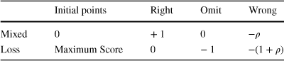
|
Initial points |
Right |
Omit |
Wrong |
|
|---|---|---|---|---|
|
Mixed |
0 |
+ 1 |
0 |
|
|
Loss |
Maximum Score |
0 |
− 1 |
|


Let
 denote the utility function of student i when receiving outcome
 from prospect j (item j). Without loss of generality, fix prospect j as the prospect being evaluated by the decision-maker. So, from now on, we refrain from using subscript j in the notation. Prospect Theory (Kahneman and Tversky Reference Kahneman and Tversky1979) assesses that decision-makers “perceive outcomes as gains and losses, rather than as final states” and “the location of the reference point, and the consequent coding of outcomes as gains or losses, can be affected by the formulation of the offered prospects” (Kahneman and Tversky Reference Kahneman and Tversky1979). According to these ideas, in our model students perceive each item as a potential gain or loss. In other words, their reference point depends on the assigned framing and corresponds to the expected score excluding the evaluated prospect.Footnote 5 According to this formulation, the argument of
 under each framing corresponds to the values presented in Table 1. Similar models have been considered in a testing context by Budescu and Bo (Reference Budescu and Bo2015) and Karle et al. (Reference Karle, Engelmann and Peitz2019).
For
 , we let
 where
where
 is twice differentiable with
 ,
,
 and
and
 . Following the widespread formulation by Kahneman and Tversky (Reference Kahneman and Tversky1979), for any
 let
let
 where
where
 is the loss-aversion parameter. A student is loss-averse if and only if
 . This formulation implies that concavity in the gain domain becomes convexity in the loss domain (Kahneman and Tversky Reference Kahneman and Tversky1979, call this phenomenon the reflection effect). Throughout the paper, we measure concavity according to Arrow-Pratt measure
 .
.
Let
 be student i’s perceived probability of choosing the correct answer with
 denoting student i’s knowledge of the topic evaluated and
 accounting for other characteristics, such as self-confidence, that may influence student i’s perceived probability of answering correctly. We assume the perceived probability
 to be independent of the particular scoring rule. To ease the exposition, we refrain from using the arguments determining the perceived probability and henceforth refer to it as
 .
.
In Prospect Theory probabilities are evaluated according to decision weights, which can differ from actual probabilities by overweighting small probabilities and underweighting moderate and large probabilities. Let
 and
and
 be the functions mapping student i’s perceived probability
 into the decision weights of correct and incorrect answers, respectively (i.e.,
 ,
,
 ). According to Prospect Theory (Kahneman and Tversky Reference Kahneman and Tversky1979), decisions weights are assumed to satisfy: i)
 and
and
 , ii)
, ii)
 and
and
 , iii)
 is increasing in
 , iv)
, iv)
 is decreasing in
 (i.e., increasing on
 ) and, v)
 . The latter assumption implies that the perceived probability of correct (
 ) and incorrect (
 ) answers can be simultaneously underweighted (i.e.,
 and
and
 ) but only one of the two can be overweighted (i.e., either
 or
or
 ).
).
Under the Mixed-framing, correct answers will result in a gain of 1 (normalized) point, wrong answers in a loss of
 points, and non-responses will receive zero points. So, a student is expected to provide an answer under the Mixed-framing if:

Since
 and
and
 are increasing and decreasing in
 , respectively, the left hand side of the latter inequality is increasing in
 . Thus, we can define
 as the minimum value for which the above inequality holds (i.e., the unique value of
 solving equation (1) with equality). Thus,
 represents the cut-off probability at which student i chooses to provide an answer under the Mixed-framing. Running comparative statics on
 we obtain the results in Lemma Footnote 1.
Lemma 1
Let
 for
for
 and
and
 for
for
 , where
 ,
,
 and
and
 . Under the Mixed-framing, non-response is increasing in the loss attitude parameter (
 ) and in the concavity of
 .
.
The proof of the lemma is in Appendix A. As
 is increasing in
 and in the concavity of
 , either loss-aversion and/or risk-aversion (in the positive domain) might be causing non-response in the Mixed-framing.
Under the Loss-framing, students are told they will start the exam with the maximum grade. Correct answers will result in no points loss, wrong answers in a loss of
 points and non-responses in a loss of 1 point. A student is expected to provide an answer if:

Similarly as before, we can define
 as the cut-off probability at which student i chooses to provide an answer under the Loss-framing.
Lemma 2
Let
 for
for
 and
and
 for
for
 , where
 ,
,
 and
and
 . Under the Loss-framing, non-response is independent from the loss attitude (
 ) and decreasing in the concavity of
 .
.
The proof of the lemma is in Appendix A. In contrast to the Mixed-framing, under Loss-framing, non-response is unaffected by loss attitude (
 ). Loss-framing eliminates the asymmetry between gains and losses that exists under Mixed-framing. As a consequence, the loss attitude does not affect non-response under Loss-framing.
At first glance, the second part of Lemma Footnote 2 might be surprising, as concavity is generally associated to a higher level of risk-aversion. However, according to Prospect Theory, this is only so in the gain domain. The reflection effect implies that “risk aversion in the positive domain is accompanied by risk seeking in the negative domain" (Kahneman and Tversky Reference Kahneman and Tversky1979). This implies that more risk-averse students in the gain domain, who are risk-seekers in the negative domain, should display lower levels of non-response under the Loss-framing.
Next, we compare the level of non-response under the two framings. As
 represents the cut-off probability at which a student chooses to provide an answer under each framing
 , a higher value indicates greater non-response, all else equal. By comparing the two cut-offs, we can obtain the following result.
Proposition 1
Let
 for
for
 and
and
 for
for
 , where
 ,
,
 and
and
 . The Loss-framing induces lower non-response if
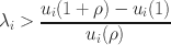
The proof is in Appendix A. Proposition Footnote 1 provides a sufficient condition for observing a reduction in non-response under the Loss-framing.
The left hand side of the expression in Proposition Footnote 1 is increasing in loss-aversion, while the right hand side is decreasing in the concavity of
 .Footnote 6 Thus, both loss-aversion and the concavity of
 can contribute to observe less omitted questions under the Loss-framing. The first effect is a consequence of canceling-out the effect of loss-aversion under the Loss-framing documented in Lemma Footnote 2. The second effect arises from the reflection effect, which makes individuals more willing to take risks when confronted with the Loss-framing. Moreover, for any degree of concavity of
 , it is always possible to find a degree of loss-aversion that induces less omitted questions under the Loss-framing (see Figure 1 for a graphic illustration).
Proposition Footnote 1 implies that mild conditions are sufficient for the Loss-framing to induce higher non-response than the Mixed-framing, as highlighted in the next corollary.
Fig. 1 Graphical illustration of Proposition Footnote 1 according to an exponential utility function (
 for
for
 ,
,
 for
for
 ) with
 and
and
 . The X-axis represents the degree of (absolute) risk aversion r. The Y-axis represents the degree of loss-aversion
 . The blue line shows the combinations of risk and loss attitudes for which
 . The area shaded in light gray shows the combination of parameters making
 and the area shaded in dark grey the combinations making

Corollary 1
Test-taker displaying simultaneously concavity of
 and loss-aversion is sufficient to observe lower non-response under the Loss-framing than under the Mixed-framing.
The proof of the corollary is in the Appendix A. Corollary Footnote 1 establishes a sufficient (but not necessary) condition for finding a positive treatment effect on response-rates. This sufficient condition is illustrated in Figure 1 where
 always holds for any combination
 (loss-aversion) and
 (concavity of
 ). Previous studies have shown that, although heterogeneous, the population displays both concavity in u(.) and loss-averse attitudes (Fishburn and Kochenberger Reference Fishburn and Kochenberger1979; Abdellaoui Reference Abdellaoui2000; Abdellaoui et al. Reference Abdellaoui, Bleichrodt and Paraschiv2007, Reference Abdellaoui, Bleichrodt and Haridon2008; Andersen et al. Reference Andersen, Harrison, Lau and Rutström2008; Booij and Van de Kuilen Reference Booij and Van de Kuilen2009; Harrison and Rutström Reference Harrison and Rutström2009; Gaechter et al. Reference Gaechter, Johnson and Herrmann2010; Von Gaudecker et al. Reference Von Gaudecker, Van Soest and Wengstrom2011), so we can expect the condition in Proposition Footnote 1 to hold more frequently than the opposite. These observations provide the theoretical background for our main hypothesis.
Hypothesis 1
Average non-response will be lower under the Loss-framing than under the Mixed-framing.
It also follows from lemmas Footnote 1 and Footnote 2 that the reduction in non-response under the Loss-framing would be greater the more risk- and loss-averse the decision-maker is.Footnote 7 This implies that women who have been found to be more risk-averse (e.g., Eckel and Grossman Reference Eckel and Grossman2002; Fehr-Duda et al. Reference Fehr-Duda, De Gennaro and Schubert2006) and more loss-averse than men (e.g., Schmidt and Traub Reference Schmidt and Traub2002; Booij et al. Reference Booij, Van Praag and Van De Kuilen2010; Rau Reference Rau2014) might exhibit a higher decrease in terms of non-responses under the Loss framing.
Next, we address the consequences of Hypothesis 1 on test performance. Let
 be student i’s actual probability of answering a specific item correctly.Footnote 8 If Hypothesis 1 is confirmed, the ratio of correct answers over the total number of questions must increase for any
 .
.
The condition for observing an increase in test scores is more demanding due to the penalties for wrong answers
 . Additional answers increase the score if and only if
 . Let
. Let
 be the number of alternatives in a test item. For all the MCTs considered in our intervention
 . By replacing the values of
 by its highest value
 in the expression for
 , we get that
 . Note that
 is the probability of answering correctly by choosing a random alternative. Thus, if Hypothesis 1 holds, a sufficient condition for an increase in test scores under the Loss-framing is that the probability that the additional answers are correct is greater than if choosing randomly. If these conditions hold, Hypothesis 2 automatically follows:
Hypothesis 2
Average scores will be higher under the Loss-framing than under the Mixed-framing.
Finally, note that an increase in the proportion of correct answers is necessary but not sufficient for observing an increase in test scores.
4 Experimental design
We conducted a field experiment with 554 students from the University of the Balearic Islands (Spain). All participants had to do a penalized MCT as a part of a course evaluation. The exams involved substantial stakes, accounting for between 20%-33% of their final course score. Test scores have important consequences for undergraduate students in terms of career prospects, grants, costly effort and tuition fees. Students’ attendance in the exams was almost 100% which confirms their importance for students.
The experiment consisted of modifying the framing of the MCT instructions. The design of the experiment was approved by the Ethics Committee of the University of the Balearic Islands under registration number 99CER19.
4.1 Treatments
The experiment consisted of modifying the framing of the exam instructions according to the score equivalent rules in Table 1. The treatments only varied in the instructions, where two framings were used to describe the scoring rule:
• Mixed-framing (control): Typical framing for a penalized MCT where each correct answer adds points to the score, omitted answers do not add or subtract points and wrong answers are penalized. Example:Footnote 9
The exam is a multiple-choice test with 20 questions and 5 possible answers for each question. Only one of the 5 potential answers is correct. The maximum grade is 100 points. Correct answers give you 5 points. Each incorrect answer subtracts 1.25 points and finally each unanswered (omitted) question does not subtract or add points. For instance, a student who answered 16 questions correctly, left 3 unanswered questions and answered 1 question incorrectly, would have a final score of 78.75 over 100 (16*5- 3*0 - 1*1.25 = 78.75).
• Loss-framing (treatment): We proposed a score equivalent manipulation of the Mixed-framing. Students were informed that they would start the test with the highest score. Correct answers would not add to or subtract anything from the initial score. Each wrong or omitted answer would decrease this initial maximum score by an amount equivalent to the one under the Mixed-framing. Example:
The exam is a multiple-choice test with 20 questions and 5 possible answers for each question. Only one of the 5 potential answers is correct. The maximum grade is 100 points. You start the exam with a grade equal to this maximum score. The correct answers do not subtract anything. Each incorrect answer will subtract 6.25 points and finally, each unanswered (omitted) question will subtract 5 points. For instance, a student who answered 16 questions correctly, left 3 unanswered questions and answered 1 question incorrectly, would have a final score of 78.75 over 100 (100-16*0- 3*5 - 1*6.25 = 78.75).
4.2 Implementation details
We conducted the field experiment in 14 different sessions. Each session related to a different exam. Within each session, half of the students were randomly assigned to the Mixed-framing and the other half to the Loss-framing. All the exams took place during the 2018-2019 academic year.Footnote 10
Table 2 presents the main features for each of the sessions. All exams in our study were part of the official evaluation of three different courses (Introduction to Business, Human Resource Management, and Business) taught by eight different members of the Department of Business Economics.Footnote 11 The exams lasted between 30 minutes and 1 hour. Stakes, penalty size, number of items and number of alternatives in each item varied slightly between exams and courses. Importantly, all were midterm exams accounting for between 20% and 33% of the final grade. None of these MCTs had a cut-off score or released material for the final exam. Thus, as in the model presented above, students should have been aiming to maximize their final scores.Footnote 12
All the students knew in advance that the exam was an MCT but they did not know the specific scoring rules. More importantly, students were not aware of the existence of different framings while doing the exam.Footnote 13 Each student participated in only one session and was only exposed to one of the two treatments.Footnote 14
Randomization was implemented in three different ways depending on organizational features of the exams. For computer-based exams, the on-line platform automatically and randomly assigned students to one of the framing conditions. In paper-based exams, hard copies of the grading instructions were delivered in such a way that immediate neighbors were assigned a different framing. This was done to ensure that the different framings were spread over the entire classroom to prevent the possibility that students’ seats were not random. Finally, in one of the courses, the treatments were assigned according to surnames in alphabetical order. Alphabetical order can be considered quasi-random. Since this course involved several sessions, to prevent surname effects, the mixed condition was implemented for the first half in alphabetical order in some sessions and for the second half in the remaining sessions.
For computer and surname-based randomization, whenever more than one classroom was available, students under the Mixed and Loss-framings took the exam in separate rooms. Students in these groups were assigned ex-ante (by the computer or their surname) to Mixed or Loss-framings and directed to take the exam in a particular room where all the other students were under the same treatment. Our aim was to avoid spillover effects. In case of taking the exam in a single classroom, an extra proctor was assigned to prevent spillovers between the different experimental conditions. Before starting the exam, students had 5 minutes to read the instructions (containing our treatments) and to privately ask any questions that they may have had regarding the evaluation method. After these 5 minutes, the exam started.
We also carried out a pilot study with 184 subjects from another course. In each exam, there were two shifts corresponding to different groups taking the course. The treatment was assigned at a group level. Despite the treatment being randomly assigned to each group, the group formation itself may not have been random. Therefore the observations from this pilot study are not included in our main results.Footnote 15
Finally, to gain better insights on the specific mechanisms driving the framing effect, we invited students to participate in an incentivized on-line survey. A total of 166 subjects who participated in the main study (30,9% of the total sample) filled in this survey. Participants were asked to complete 5 different incentivized tasks designed to measure their risk and loss preferences (see Appendix D for more information on the specific tasks). We present the survey and its results on Section 6.
Table 2 Description of the sessions/exams
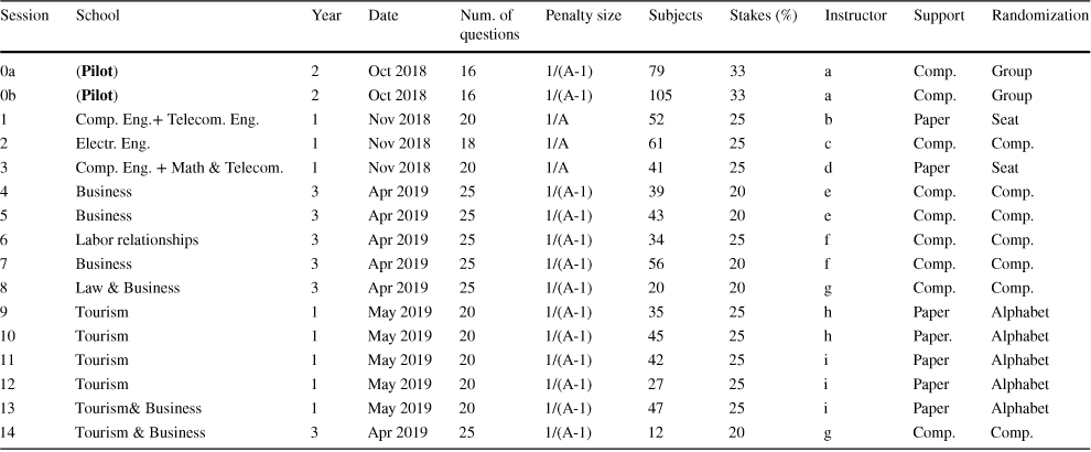
|
Session |
School |
Year |
Date |
Num. of questions |
Penalty size |
Subjects |
Stakes (%) |
Instructor |
Support |
Randomization |
|---|---|---|---|---|---|---|---|---|---|---|
|
0a |
(Pilot) |
2 |
Oct 2018 |
16 |
1/(A-1) |
79 |
33 |
a |
Comp. |
Group |
|
0b |
(Pilot) |
2 |
Oct 2018 |
16 |
1/(A-1) |
105 |
33 |
a |
Comp. |
Group |
|
1 |
Comp. Eng.+ Telecom. Eng. |
1 |
Nov 2018 |
20 |
1/A |
52 |
25 |
b |
Paper |
Seat |
|
2 |
Electr. Eng. |
1 |
Nov 2018 |
18 |
1/A |
61 |
25 |
c |
Comp. |
Comp. |
|
3 |
Comp. Eng. + Math & Telecom. |
1 |
Nov 2018 |
20 |
1/A |
41 |
25 |
d |
Paper |
Seat |
|
4 |
Business |
3 |
Apr 2019 |
25 |
1/(A-1) |
39 |
20 |
e |
Comp. |
Comp. |
|
5 |
Business |
3 |
Apr 2019 |
25 |
1/(A-1) |
43 |
20 |
e |
Comp. |
Comp. |
|
6 |
Labor relationships |
3 |
Apr 2019 |
25 |
1/(A-1) |
34 |
25 |
f |
Comp. |
Comp. |
|
7 |
Business |
3 |
Apr 2019 |
25 |
1/(A-1) |
56 |
20 |
f |
Comp. |
Comp. |
|
8 |
Law & Business |
3 |
Apr 2019 |
25 |
1/(A-1) |
20 |
20 |
g |
Comp. |
Comp. |
|
9 |
Tourism |
1 |
May 2019 |
20 |
1/(A-1) |
35 |
25 |
h |
Paper |
Alphabet |
|
10 |
Tourism |
1 |
May 2019 |
20 |
1/(A-1) |
45 |
25 |
h |
Paper. |
Alphabet |
|
11 |
Tourism |
1 |
May 2019 |
20 |
1/(A-1) |
42 |
25 |
i |
Paper |
Alphabet |
|
12 |
Tourism |
1 |
May 2019 |
20 |
1/(A-1) |
27 |
25 |
i |
Paper |
Alphabet |
|
13 |
Tourism& Business |
1 |
May 2019 |
20 |
1/(A-1) |
47 |
25 |
i |
Paper |
Alphabet |
|
14 |
Tourism & Business |
3 |
Apr 2019 |
25 |
1/(A-1) |
12 |
20 |
g |
Comp. |
Comp. |
Notes: Pilot was not within group randomized and is excluded from main estimations. Regarding randomization, alphabetical order is considered quasi-random but not-random. To prevent surname effects the treatment condition was implemented to first half of students in alphabetical order in sessions 10, 12 and to second half for sessions 9, 11, 13. In session 14 one student made a question referencing the grading system aloud compromising the validity of the data for that session
4.3 Data and descriptive statistics
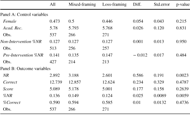
Our main sample consisted of 537 students.Footnote 16 266 students (49.53%) were assigned to the Mixed-framing and 271 (50.47%) to the Loss-framing. We observed their score in the test (Score), their total number of omitted questions (NR), the total number of correct answers (Correct), and the corresponding proportions (%NR and %Correct). We were also granted access to administrative data from the University of the Balearic Islands, including students’ academic record on a 0 to 10 scale (Acad. Rec.) and gender (Female). All data used in this study was conveniently anonymized by the IT services of the university.Footnote 17 To further check that the randomization worked correctly, we also retrieved information on test takers’ non-response from different computer-based MCTs other than the ones in the experiment (Non-Intervention %NR). These data were obtained from other exams performed during the 2018-2019 academic year and were available for 513 out of the 537 participating students.Footnote 18 We also constructed a pre-intervention non-response measure but in this case, we could only gather data for 427 students (80% of our sample).
Table 3 shows the overall average of our main variables (column 1) and the average for the Mixed-framing and Loss-framing (columns 2 and 3). It also shows the difference between treatments (column 4), standard errors (column 5), and the p-value for the two-sample t-test on means equality (column 6). Overall, Panel A in Table 3 shows no difference in gender composition or academic record between the students exposed to the Mixed and Loss-framings. More importantly, groups are also balanced in terms of non-response in tests outside the intervention, which can be considered a placebo test of our treatment (a proper placebo test is provided in Table B5 of Appendix B). Table B1 in Appendix B reports descriptive statistics by session. Though a few exceptions arise, treatment and control were balanced according to most of the observables at the session level. When presenting our results, we show they are robust when excluding sessions where any of the observables were not balanced between control and treatment. Taking all this together, we find support for our claim that randomization worked properly and that both groups are comparable ex-ante.
Table 3 Descriptive Statistics
|
All |
Mixed-framing |
Loss-framing |
Diff. |
Std.error |
p-value |
|
|---|---|---|---|---|---|---|
|
Panel A: Control variables |
||||||
|
Female |
0.473 |
0.5 |
0.446 |
0.054 |
0.043 |
0.215 |
|
Acad. Rec. |
5.78 |
5.793 |
5.768 |
0.026 |
0.120 |
0.831 |
|
Obs. |
537 |
266 |
271 |
|||
|
Non-Intervention %NR |
0.127 |
0.127 |
0.127 |
0.001 |
0.013 |
0.950 |
|
Obs. |
513 |
256 |
257 |
|||
|
Pre-Intervention %NR |
0.141 |
0.135 |
0.147 |
− 0.012 |
0.017 |
0.484 |
|
Obs. |
427 |
214 |
213 |
|||
|
Panel B: Outcome variables |
||||||
|
NR |
2.892 |
3.188 |
2.601 |
0.586 |
0.191 |
0.0023 |
|
Correct |
12.739 |
12.857 |
12.624 |
0.234 |
0.329 |
0.4787 |
|
Score |
5.089 |
5.178 |
5.001 |
0.177 |
0.158 |
0.2639 |
|
%NR |
0.136 |
0.149 |
0.124 |
0.025 |
0.0089 |
0.0059 |
|
%Correct |
0.590 |
0.594 |
0.585 |
0.01 |
0.0132 |
0.4736 |
|
Obs. |
537 |
266 |
271 |
|||
Female takes value 1 when the student is female and 0 otherwise. Acad. Rec. is the grade point average (GPA) of the student in the degree. Non-Intervention %NR is the average percentage of items omitted in other MCT different to the one of the intervention during the academic year 18-19. Non-Intervention %NR (Before the intervention) is the average percentage of items omitted in other MCT in the academic year 18-19 taking place before the intervention. NR (%NR) is the number (percentage) of omitted questions in the experiment. Correct (%Correct) is the number (percentage) of correct answers provided in the intervened exam. Score is the final grade in the intervened exam
Panel B in Table 3 presents the comparison between the Mixed and the Loss-framings for our main outcome variables. Raw averages show that non-response is significantly lower under the Loss than under the Mixed-framing both in total number (p-value=0.002) and as a percentage of the total number of questions in the exam (p-value=0.006). In other words, students under the Loss-framing answered more questions on average than students under the Mixed-framing. This finding is in line with our Hypothesis 1. By contrast, we find no evidence in favor of Hypothesis 2. When looking at the variable Score, we observe that the difference, although not significant, has the opposite sign to that predicted in Hypothesis 2. The same happens with the number and the proportion of correct answers.
In the next section, we present ordinary least squares (OLS) estimates of the treatment effect to provide a more accurate analysis by adding session-fixed effects and students’ controls. In what follows, results will be presented in terms of the non-response rate (% NR) but results are qualitatively the same by using the total number of omitted items.Footnote 19
5 Results
Firstly, we focus on the framing effects on risk-taking decisions by using the non-response rate as a (negative) measure of risk-taking. Then, we analyze the framing effects on performance (test scores and proportion of correct answers).
5.1 Treatment effect on non-response
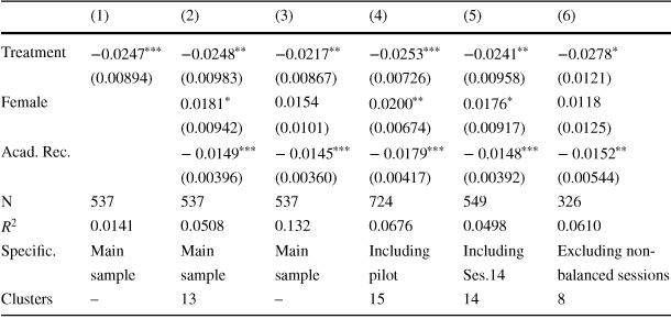
Table 4 reports the effects of the intervention on the non-response rate estimated by OLS. Changing from the Mixed-framing to the Loss-framing reduces the non-response rate. Column 1 does not control for group fixed effects. Without controlling for the specifics of each session, we found that non-response reduces by 2.47 percentage points under the intervention. In relative terms, changing the framing reduces non-response by 18.28%.
Table 4 OLS estimation of treatment effects on non-response (% NR)
|
(1) |
(2) |
(3) |
(4) |
(5) |
(6) |
|
|---|---|---|---|---|---|---|
|
Treatment |
−0.0247
|
−0.0248
|
−0.0217
|
−0.0253
|
−0.0241
|
−0.0278
|
|
(0.00894) |
(0.00983) |
(0.00867) |
(0.00726) |
(0.00958) |
(0.0121) |
|
|
Female |
0.0181
|
0.0154 |
0.0200
|
0.0176
|
0.0118 |
|
|
(0.00942) |
(0.0101) |
(0.00674) |
(0.00917) |
(0.0125) |
||
|
Acad. Rec. |
− 0.0149
|
− 0.0145
|
− 0.0179
|
− 0.0148
|
− 0.0152
|
|
|
(0.00396) |
(0.00360) |
(0.00417) |
(0.00392) |
(0.00544) |
||
|
N |
537 |
537 |
537 |
724 |
549 |
326 |
|
|
0.0141 |
0.0508 |
0.132 |
0.0676 |
0.0498 |
0.0610 |
|
Specific. |
Main |
Main |
Main |
Including |
Including |
Excluding non- |
|
sample |
sample |
sample |
pilot |
Ses.14 |
balanced sessions |
|
|
Clusters |
– |
13 |
– |
15 |
14 |
8 |


Notes: All regressions include session fixed effects except column 1. Standard errors (in parentheses) clustered at session level, except for columns 1 (robust standard errors) and 3 (a robust to outliers estimation using rreg command in Stata).

 ,
,

 ,
,


In subsequent columns, we add controls, session-fixed effects, and clustered standard errors at the exam level. By adding session-fixed effects, we are also controlling for language of the test, lecturers, degree, and subject. We consider this to be the most suitable specification for our model. Standard errors were corrected for heteroskedasticity and clustered at the session level to account for potential intra-group correlation.Footnote 20 Considering the fractional nature of our dependent variable, as a robustness check we replicated the above results following the method proposed by Papke and Wooldridge (Reference Papke and Wooldridge1996). Results remain the same (see Table B4 in Appendix B).
The size of the treatment effect and statistical significance remains comparable when adding group fixed effects, gender, and academic record controls (column 2). Column 3 provides an estimate which is robust to outliers and slightly reduces the size of the treatment effect.Footnote 21 Columns 4 and 5 add the data obtained in the two pilot sessions and in session 14 (the potentially contaminated session), respectively. Finally, Column 6 excludes the groups for which we found any statistically significant difference (10% level) in the balancing tests displayed in Table B1 in Appendix B. The result holds for all specifications.
As an additional robustness check, we conducted a placebo test considering session-homogeneous measures for out-of-intervention non-response (see Table B5 in Appendix B). This placebo test confirms that students under the Mixed and Loss-framing were comparable in out-of-intervention non-response.
In line with previous literature, we also observe that women tend to skip slightly more questions than men. Despite the subtle change in the instructions, in our sample, the change induced in non-response is larger than the highly studied gender differences in non-response. Finally, non-response is lower for students with better academic records. In terms of our model, this may be explained if the perceived probability of providing a correct answer increases with knowledge, which could be proxied by academic record.
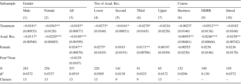
5.1.1 Heterogeneous effects on non-response
Table 5 OLS estimation of heterogeneous treatment effects on non-response (% NR)
|
Subsample |
Gender |
Tier of Acad. Rec. |
Course |
|||||||
|---|---|---|---|---|---|---|---|---|---|---|
|
Male |
Female |
All |
Lower |
Second |
Third |
Upper |
Business |
HHRR |
Introd |
|
|
(1) |
(2) |
(3) |
(4) |
(5) |
(6) |
(7) |
(8) |
(9) |
(10) |
|
|
Treatment |
−0.0181* |
−0.0363** |
−0.0187* |
−0.0273* |
−0.0161* |
−0.0278* |
−0.0216 |
−0.00237 |
−0.0512*** |
−0.0182 |
|
(0.00933) |
(0.0120) |
(0.00877) |
(0.0160) |
(0.00921) |
(0.0165) |
(0.0220) |
(0.0140) |
(0.0136) |
(0.0160) |
|
|
Acad. Rec. |
−0.0117* |
−0.0220*** |
−0.0149*** |
-0.00953** |
-0.0246*** |
-0.0158** |
||||
|
(0.00540) |
(0.00485) |
(0.00399) |
(0.00461) |
(0.00666) |
(0.00742) |
|||||
|
Female |
0.0247** |
0.0275* |
0.0183 |
0.0171** |
0.00197 |
-0.00555 |
0.0238 |
0.0236 |
||
|
(0.00870) |
(0.0165) |
(0.0191) |
(0.00706) |
(0.0189) |
(0.0230) |
(0.0146) |
(0.0170) |
|||
|
Fem*Treat |
−0.0129 |
|||||||||
|
(0.0107) |
||||||||||
|
N |
283 |
254 |
537 |
220 |
141 |
91 |
85 |
152 |
190 |
195 |
|
|
0.0372 |
0.0727 |
0.0519 |
0.0305 |
0.0138 |
0.0323 |
0.0172 |
0.0296 |
0.130 |
0.0372 |
|
Clusters |
13 |
13 |
13 |
13 |
9 |
9 |
13 |
– |
– |
– |

Notes: All regressions include session fixed effects except for columns 8 to 10. Standard errors (in parentheses) are clustered at session level, except in columns 8 to 10.

 ,
,

 ,
,


Now we explore the heterogeneous treatment effects for different groups of students. The size of the treatment effect is two times larger for women (Column 1 restricted for men and 2 for women in Table 5). However, by interacting the gender and treatment dummies in Column 3, we did not find any sufficiently strong evidence to claim that framing induces differential effects across genders. Nevertheless, gender effects may be attenuated by the highly unbalanced composition of some sessions (STEM degrees).
Columns 4-7 divide our sample according to students’ academic record.Footnote 22 The treatment effect is similar and significant across the different tiers of academic record, with the exception of the highest level. Non-response is already very small for students at the highest level of academic record (notice the negative coefficient for academic record in all our specifications in Table 4), which may explain their lower reaction to the treatment. Also, the group with the highest academic record is the smallest, so it might also be a matter of power.
In Columns 8-10, we report separate estimates for each of the courses evaluated in our sample. An interesting pattern emerges. The biggest effect arises from “Human Resource Management” (Column 9). We find the smallest one for “Business”, a course that was taught to engineers. Engineers seem to be unaffected by the treatment. Finally, Column 10 does not display statistically significant effects for the course “Introduction to Business” taught to students in the Business and Tourism schools. However, this non-significance seems to be driven by session 10, in which the control group was displaying statistically significant (5%) lower non-response before the treatment (see Table B1). The framing effect becomes statistically significant for “Introduction to Business” when that group is dropped.
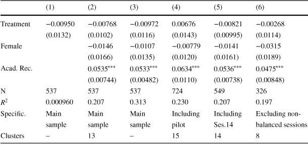
5.2 Treatment effect on performance
Hypothesis 2 predicts that test scores increase under the Loss-framing. This is especially likely to hold, after observing that the treatment increases students’ response rate.
Table 6 OLS estimation of treatment effects on correct answers (% Correct)
|
(1) |
(2) |
(3) |
(4) |
(5) |
(6) |
|
|---|---|---|---|---|---|---|
|
Treatment |
−0.00950 |
−0.00768 |
−0.00972 |
0.00676 |
−0.00821 |
−0.00268 |
|
(0.0132) |
(0.0102) |
(0.0116) |
(0.0143) |
(0.00995) |
(0.0114) |
|
|
Female |
−0.0146 |
−0.0107 |
−0.00779 |
−0.0141 |
−0.0315 |
|
|
(0.0166) |
(0.0135) |
(0.0120) |
(0.0161) |
(0.0189) |
||
|
Acad. Rec. |
0.0535
|
0.0533
|
0.0634
|
0.0536
|
0.0475
|
|
|
(0.00744) |
(0.00482) |
(0.0110) |
(0.00738) |
(0.00848) |
||
|
N |
537 |
537 |
537 |
724 |
549 |
326 |
|
|
0.000960 |
0.207 |
0.313 |
0.230 |
0.207 |
0.197 |
|
Specific. |
Main |
Main |
Main |
Including |
Including |
Excluding non- |
|
sample |
sample |
sample |
pilot |
Ses.14 |
balanced sessions |
|
|
Clusters |
– |
13 |
– |
15 |
14 |
8 |


Notes: All regressions include session fixed effects except column 1. Standard errors (in parentheses) clustered at session level, except for columns 1 (robust standard errors) and 3 (robust to outliers estimation using rreg command in Stata).

 ,
,

 ,
,


Table 6 contains the same specifications as Table 4 but using correct answers as the dependent variable. Remember that an increase in the proportion of correct answers is a necessary but not sufficient condition for an increase in test scores. Table 6 rejects Hypothesis 2. The treatment does not have a positive effect on the proportion of correct answers, so it cannot increase test scores (see Table B6 in the Appendix for the results on test scores). Even more strikingly, despite not being statistically significant, the treatment coefficient has the opposite sign than the one expected.
This result is surprising because, as omitted items are surely not correct, increasing the response rate has a positive mechanical effect on correct answers. This mechanical effect can be defined as:

Where
 is the average probability of answering correctly in marginal responses and
 is the framing effect on non-response. We know from Table 4 that
 , while by definition
 .
.
The mechanical effect implies that if the Loss-framing only affects performance throughout the change induced in non-response, then we cannot observe a negative effect on correct answers and indeed we might observe a positive effect if
 . These observations are at odds with the results in Table 4.
Indeed, if the Loss-framing only affects performance throughout the change induced in non-response, the results in Tables 4 and 6 can only be reconciled if
 is negative.Footnote 23 Despite being not-statistically significant, the negative coefficients are unfeasible and imply that the change in framing affected performance by a channel other than non-response. In other words, students under the Loss-framing seem to experience worse overall performance.
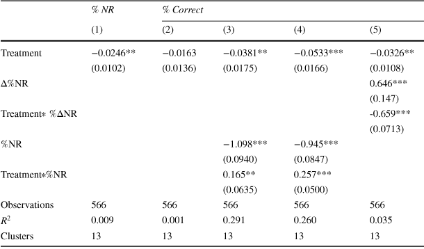
The main difficulty in analyzing the possibility of impaired performance relies on the existence of the mechanical effect described above. The mechanical effect and impaired performance work in opposite directions. Thus, the two effects may cancel each other out and result in a non-statistically significant effect on correct answers as in Table 6. However, by exploiting question-level data, we can partial-out the mechanical effect to further explore the possibility of impaired performance. To do so, we focus on those questions where the change induced in non-response by the treatment is small and, consequently, the mechanical effect is shut down or, at least, substantially reduced. These items offer the possibility of analyzing impaired performance after partialling out the mechanical effect.Footnote 24 The results of this analysis are presented in Table 7.
Table 7 OLS estimation for the Question Level Analysis
|
% NR |
% Correct |
||||
|---|---|---|---|---|---|
|
(1) |
(2) |
(3) |
(4) |
(5) |
|
|
Treatment |
−0.0246** |
−0.0163 |
−0.0381** |
−0.0533*** |
−0.0326** |
|
(0.0102) |
(0.0136) |
(0.0175) |
(0.0166) |
(0.0108) |
|
|
|
0.646*** |
||||
|
(0.147) |
|||||
|
Treatment
|
-0.659*** |
||||
|
(0.0713) |
|||||
|
%NR |
−1.098*** |
−0.945*** |
|||
|
(0.0940) |
(0.0847) |
||||
|
Treatment
|
0.165** |
0.257*** |
|||
|
(0.0635) |
(0.0500) |
||||
|
Observations |
566 |
566 |
566 |
566 |
566 |
|
|
0.009 |
0.001 |
0.291 |
0.260 |
0.035 |
|
Clusters |
13 |
13 |
13 |
13 |
13 |


Notes: Regressions at the question level for %NR in column 1 and for % Correct in columns 2-5. %NR computed as the total non-response rate in column 3 and as the non-response rate of students in the Mixed-treatment only in column 4. All regressions include session fixed effects. Standard errors clustered at session level in parentheses.

 ,
,

 ,
,


Columns 1 and 2 in Table 7 replicate the above results on framing effects using question-level data. Column 1 confirms that the Loss-framing reduces non-response by 2.4 percentage points while column 2 shows that it has a negative but not significant effect on correct answers. In columns 3, 4, and 5 we use the percentage of correct answers as the dependent variable and add explanatory variables intended to capture the mechanical effect and their interaction with the treatment dummy. Consequently, the uninteracted treatment dummy provides the coefficient of interest: the framing effect on the items where the mechanical effect is more likely to be inactive.
We use three different approaches to identify items where the mechanical effect is weaker. In columns 3 and 4, we exploit a natural cap on the mechanical effect. For items where non-response is close to zero, changing to the Loss-framing cannot further reduce non-response. Following this logic, in these two columns, we add the non-response rate as a regressor and its interaction with the treatment dummy. In column 3, the non-response rate was calculated using all subjects, while in column 4 it was calculated using only the control group (Mixed-framing).Footnote 25 Given that we are controlling for the proportion of non-response and its interaction with the treatment, the (uninteracted) treatment dummy provides an estimate on the framing effect for the questions where non-response was close to zero. In the two cases, this coefficient of interest is negative and statistically significant, thereby providing evidence of impaired performance on those items where the mechanical effect is inactive. In column 5, instead of using an exogenous cap, we directly consider the observed difference in non-response (
 ) for each test item j. The result is very similar to the ones in columns 3 and 4. The coefficients of the (uninteracted) treatment dummies are negative and statistically significant, showing evidence of impaired performance on those items where the mechanical effect is capped.
Impaired performance explains why in Table 6 we found that, despite answering more items, students under the Loss-framing did not get a higher percentage of correct answers and why we get a negative but not significant result: Students provide more answers under the Loss-framing but all answers, including the ones to the items that would have been answered even in the absence of the treatment, are of poorer quality.
6 Risk-aversion vs loss-aversion
Table 8 Treatment effects interacted with risk and loss attitude (% NR)
|
(1) |
(2) |
(3) |
(4) |
(5) |
(6) |
(7) |
(8) |
|
|---|---|---|---|---|---|---|---|---|
|
Treatment |
−0.0411
|
−0.123
|
-0.0526 |
-0.0713
|
-0.0609 |
−0.0401
|
−0.0403
|
−0.0584 |
|
(0.0211) |
(0.0381) |
(0.0335) |
(0.0313) |
(0.0539) |
(0.0210) |
(0.0202) |
(0.0511) |
|
|
SOEP |
0.00724
|
|||||||
|
(0.00386) |
||||||||
|
Treat
|
−0.0142
|
|||||||
|
(0.00589) |
||||||||
|
OLST |
0.00521 |
|||||||
|
(0.00912) |
||||||||
|
Treat
|
−0.00467 |
|||||||
|
(0.0107) |
||||||||
|
NOLST |
0.00747 |
|||||||
|
(0.00624) |
||||||||
|
Treat
|
−0.0121
|
|||||||
|
(0.00587) |
||||||||
|
BRET |
0.000642 |
|||||||
|
(0.000451) |
||||||||
|
Treat
|
−0.000490 |
|||||||
|
(0.00110) |
||||||||
|
Principal Component |
0.0171
|
|||||||
|
(0.00902) |
||||||||
|
Treat
|
−0.0224
|
|||||||
|
(0.0112) |
||||||||
|
COLST |
0.00277 |
|||||||
|
(0.00390) |
||||||||
|
Treat
|
−0.00717 |
|||||||
|
(0.00735) |
||||||||
|
NPOLST |
0.0168 |
|||||||
|
(0.0138) |
||||||||
|
Treat
|
0.00426 |
|||||||
|
(0.0272) |
||||||||
|
Other controls |
YES |
YES |
YES |
YES |
YES |
YES |
YES |
YES |
|
N |
166 |
166 |
166 |
166 |
166 |
166 |
166 |
140 |
|
|
0.0945 |
0.117 |
0.0979 |
0.107 |
0.104 |
0.117 |
0.1 |
0.142 |
|
Clusters |
13 |
13 |
13 |
13 |
13 |
13 |
13 |
13 |


Notes: SOEP refers to the self-reported measure of attitude toward risk (Dohmen et al. Reference Dohmen, Falk, Huffman, Sunde, Schupp and Wagner2005). OLST refers to Ordered Lottery Selection Task (Eckel and Grossman Reference Eckel and Grossman2002). NOLST refers to Negative Ordered Lottery Selection Task which is equivalent to OLST but in the loss domain. BRET refers to the Bomb Risk Elicitation Task (Crosetto and Filippin Reference Crosetto and Filippin2013). Principal Component refers to the first factor of the principal component analysis with loads 0.501 for SOEP, 0.614 OLST, 0.489 for NOLST, and 0.333 for BRET. COLST refers to Change in Ordered Lottery Selection Task and is computed as the difference NOLST and OLST. NPOLST refers to Negative and Positive Ordered Lottery Selection Task (Gaechter et al. Reference Gaechter, Johnson and Herrmann2010) considering only consistent subjects (see Appendix D). For all measures greater values indicate greater risk or loss aversion. See Appendix D for further details in each of the measures. Other controls include Female, Acad. Rec., and session fixed effects. Clustered standard errors at the session level in parentheses.

 ,
,

 ,
,


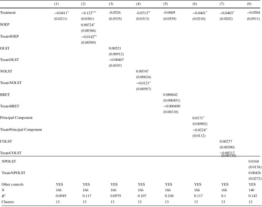
To gain better insights into the relative importance of risk and loss-aversion, we administered an incentivized survey. In this survey, students had to choose between different gambles that were specifically designed to measure their risk and loss attitudes (see Appendix D for a detailed description of each measure). Incentives were introduced by means of a lottery, where the winner effectively participated in the gamble and was paid according to his/her choices. Survey participation was voluntarily. Therefore, unfortunately, our sample reduces to 166 subjects (30.9% of the total sample) when these measures are taken into account. This restriction imposes a challenge in terms of the representativeness and power of this part of the study. Finally, we must recognize that obtaining separate measures for risk and loss-aversion can be problematic. These difficulties call for some caution when considering these results.
We collected 4 measures for risk-aversion, one for loss-aversion and one trying to capture reflection. We combined all 4 measures for risk aversion into one factor by using principal component analysis accounting for 41% of the variance. All these variables are codified such that greater values indicate greater risk or loss-aversion. Table 8 analyzes the effects of each of the measures on the treatment effect on non-response.
Firstly, none of the measures have a statistically significant effect on non-response (except for the self-reported measure and the factor that combines all four measures of risk). However, the sign of the coefficients is consistent with more risk-averse and/or loss-averse students omitting more questions under the Mixed-framing. Interestingly, we obtain statistically significant results for the interaction between the treatment (Loss-framing) and the risk-aversion measures but not for loss-aversion or reflection effect. In particular, all interaction terms with risk-aversion measures (three out of five being significant) present a negative point estimate, implying that the Loss-framing is more effective in reducing non-response among those students who are more risk-averse.
7 Conclusions
We ran a field experiment to analyze framing effects in penalized MCTs. Our intervention consisted of modifying the framing of rewards and penalties in real stakes MCTs that accounts for between 20% and 33% of students’ course grade. Under the Mixed-framing, the scoring rule was presented in a mixed gain and loss domain, while under the Loss-framing, the scoring rule was presented in the loss domain. Consistent with our theoretical predictions, we showed that non-response is greater under the Mixed than under the Loss-framing. By contrast, we did not find a positive effect on test scores or correct answers. We show that it is very plausible that students’ performance was indeed impaired under the Loss-framing.
Our paper contributes to generalizing framing effects on risk-taking from the lab to the field. However, the question of whether this result can be extended to other population groups remains open. Subjects participating in our experiment were higher education students performing a high stakes task. If we consider that high skills and stakes make decision-making more likely to be rational, then we can expect similar effects to hold in more general population. However, this is of course an open question that can only be answered by conducting more experiments of this type.
Despite our experiment not being able to identify the specific mechanism driving impaired performance, several previously documented mechanisms could be behind this finding. Higher education tests may have important and sometimes non-reversible consequences for the test taker. Students facing loss conditions may be exposed to higher levels of anxiety when they encounter unexpected evaluation methods. The link between loss framings and physical responses that indicate arousal or anxiety is well documented (Sokol-Hessner et al. Reference Sokol-Hessner, Hsu, Curley, Delgado, Camerer and Phelps2009; Hochman and Yechiam Reference Hochman and Yechiam2011; Hartley and Phelps Reference Hartley and Phelps2012), as it appears that higher anxiety levels can produce poor academic performance (Cassady and Johnson Reference Cassady and Johnson2002; Chapell et al. Reference Chapell, Blanding, Silverstein, Takahashi, Newman, Gubi and McCann2005). In addition, loss-averse subjects might perceive a greater importance of performing well under the Loss than under the Mixed-framing. If so, loss-averse subjects may choke under the extra pressure imposed by the Loss-framing, lowering their performance (Baumeister Reference Baumeister1984; Chib et al. Reference Chib, De Martino, Shimojo and O’Doherty2012).Footnote 26 Another plausible explanation is that by altering the instructions under the Loss-framing treatment, subjects may have suffered the effects of a cognitive load (Sweller et al. Reference Sweller, Van Merrienboer and Paas1998), thereby limiting their working memory and consequently impairing their performance (Baddeley Reference Baddeley1992; Carpenter et al. Reference Carpenter, Graham and Wolf2013; Deck and Jahedi Reference Deck and Jahedi2015). All these explanations are especially appealing when considering that the task performed by subjects is a one-shot cognitively demanding task where cognitive aspects, rather than effort and/or motivation, are key when it comes to determining performance. By contrast, these explanations might be irrelevant for non-cognitive or routine tasks. A limitation of the present study is its inability to find the exact mechanism that causes impaired performance. Indeed, this effect was unexpected, and our experiment was not designed to find the exact mechanism that drives it.Footnote 27
We conclude by listing the implications of our study in terms of MCT design. Loss framing in the instructions of a penalized MCT increases test takers response rate by reducing the influence of non-cognitive traits such as risk- or loss-aversion. Thus, it may provide a more accurate measure of knowledge on the evaluated topic. However, loss framing may also have unintended consequences on students’ performance. This possibility calls for some caution in scoring rule modifications. Further research on this topic might provide better insights on the reasons behind these negative effects.
Funding
Open Access funding provided thanks to the CRUE-CSIC agreement with Springer Nature.


 ui(x)=1-e-r·xr
 r≠0
r≠0 ui(x)=x
 r=0
r=0 ρ=0.25
 πiw(p~i)=1-πic(p~i)
 λ
λ p¯iMix=p¯iLoss
 p¯iMix and the area shaded in dark grey the combinations making
  p¯iMix>p¯iLoss


 Open access