


1 Introduction
Buoyancy-driven convection in porous media is a key environmental and technological process, with applications ranging from carbon dioxide storage in terrestrial aquifers to the design of compact heat exchangers (Phillips Reference Phillips1991, Reference Phillips2009; Metz et al.
Reference Metz, Davidson, de Coninck, Loos and Meyer2005; Nield & Bejan Reference Nield and Bejan2013). Porous medium convection (PMC) between plane parallel boundaries has been investigated since the 1940s, in part owing to its relative simplicity when compared with Rayleigh–Bénard convection of a pure fluid. In a sufficiently wide horizontal porous layer uniformly heated from below and cooled from above, convection sets in via a stationary bifurcation of the conduction solution at a critical Rayleigh number
 $Ra=4\unicode[STIX]{x03C0}^{2}$
, above which the layer becomes linearly unstable (Horton & Rogers Reference Horton and Rogers1945; Lapwood Reference Lapwood1948). In a two-dimensional (2D) domain, and for
$Ra=4\unicode[STIX]{x03C0}^{2}$
, above which the layer becomes linearly unstable (Horton & Rogers Reference Horton and Rogers1945; Lapwood Reference Lapwood1948). In a two-dimensional (2D) domain, and for
 $4\unicode[STIX]{x03C0}^{2}<Ra\lesssim 400$
, the convective flow manifests as steady
$4\unicode[STIX]{x03C0}^{2}<Ra\lesssim 400$
, the convective flow manifests as steady
 $\mathit{O}(1)$
aspect-ratio roll cells, each with a horizontal scale roughly equal to the layer thickness. For
$\mathit{O}(1)$
aspect-ratio roll cells, each with a horizontal scale roughly equal to the layer thickness. For
 $Ra\gtrsim 400$
, small-scale plumes, born in a supercritical Hopf bifurcation of the steady roll state, arise within the thermal boundary layers and are periodically advected around the cells by the large-scale rolls (Schubert & Straus Reference Schubert and Straus1982; Aidun & Steen Reference Aidun and Steen1987; Graham & Steen Reference Graham and Steen1992, Reference Graham and Steen1994). Following a series of transitions between periodic and quasiperiodic convective roll motions in the moderate-
$Ra\gtrsim 400$
, small-scale plumes, born in a supercritical Hopf bifurcation of the steady roll state, arise within the thermal boundary layers and are periodically advected around the cells by the large-scale rolls (Schubert & Straus Reference Schubert and Straus1982; Aidun & Steen Reference Aidun and Steen1987; Graham & Steen Reference Graham and Steen1992, Reference Graham and Steen1994). Following a series of transitions between periodic and quasiperiodic convective roll motions in the moderate-
 $Ra$
regime
$Ra$
regime
 $400\lesssim Ra\lesssim 1300$
(Kimura, Schubert & Straus Reference Kimura, Schubert and Straus1986, Reference Kimura, Schubert and Straus1987; Aidun & Steen Reference Aidun and Steen1987; Graham & Steen Reference Graham and Steen1992, Reference Graham and Steen1994), the large-scale cellular flow pattern is completely broken down for
$400\lesssim Ra\lesssim 1300$
(Kimura, Schubert & Straus Reference Kimura, Schubert and Straus1986, Reference Kimura, Schubert and Straus1987; Aidun & Steen Reference Aidun and Steen1987; Graham & Steen Reference Graham and Steen1992, Reference Graham and Steen1994), the large-scale cellular flow pattern is completely broken down for
 $Ra\gtrsim 1300$
. At sufficiently high
$Ra\gtrsim 1300$
. At sufficiently high
 $Ra$
, the flow self-organises into spatiotemporally chaotic, narrowly spaced columnar plumes (Otero et al.
Reference Otero, Dontcheva, Johnston, Worthing, Kurganov, Petrova and Doering2004; Hewitt, Neufeld & Lister Reference Hewitt, Neufeld and Lister2012; Wen, Corson & Chini Reference Wen, Corson and Chini2015b
).
$Ra$
, the flow self-organises into spatiotemporally chaotic, narrowly spaced columnar plumes (Otero et al.
Reference Otero, Dontcheva, Johnston, Worthing, Kurganov, Petrova and Doering2004; Hewitt, Neufeld & Lister Reference Hewitt, Neufeld and Lister2012; Wen, Corson & Chini Reference Wen, Corson and Chini2015b
).
In many practical applications, however, the layer may not be strictly horizontal. In carbon sequestration, for example, underground saline aquifers may be inclined with respect to the horizontal (MacMinn & Juanes Reference MacMinn and Juanes2013; Tsai, Riesing & Stone Reference Tsai, Riesing and Stone2013). Hence, it is of interest to investigate how the flow structure and transport properties are modified for convection in inclined porous layers. Consider a sloping three-dimensional (3D) porous layer with an inclination angle
 $\unicode[STIX]{x1D719}$
above the horizontal (see figure 1
a). Numerous experimental and numerical studies have revealed four types of flow near the onset of convection: the basic unicellular (shear) flow with an upward current near the lower (heated) wall and a downward current near the upper (cooled) wall; polyhedral cells with generating axes in the wall-normal (
$\unicode[STIX]{x1D719}$
above the horizontal (see figure 1
a). Numerous experimental and numerical studies have revealed four types of flow near the onset of convection: the basic unicellular (shear) flow with an upward current near the lower (heated) wall and a downward current near the upper (cooled) wall; polyhedral cells with generating axes in the wall-normal (
 $z$
) direction; longitudinal helicoidal cells resulting from the superposition of longitudinal rolls (with axes parallel to the sloping walls, i.e. to the
$z$
) direction; longitudinal helicoidal cells resulting from the superposition of longitudinal rolls (with axes parallel to the sloping walls, i.e. to the
 $x$
axis in this investigation) and the basic flow; and
$x$
axis in this investigation) and the basic flow; and
 $y$
-independent (2D) transverse rolls (Caltagirone, Cloupeau & Combarnous Reference Caltagirone, Cloupeau and Combarnous1971; Bories, Combarnous & Jaffrenou Reference Bories, Combarnous and Jaffrenou1972; Bories & Monferran Reference Bories and Monferran1972; Kaneko Reference Kaneko1972; Bories & Combarnous Reference Bories and Combarnous1973; Kaneko, Mohtadi & Aziz Reference Kaneko, Mohtadi and Aziz1974; Caltagirone & Bories Reference Caltagirone and Bories1985). The experimental studies indicate that for
$y$
-independent (2D) transverse rolls (Caltagirone, Cloupeau & Combarnous Reference Caltagirone, Cloupeau and Combarnous1971; Bories, Combarnous & Jaffrenou Reference Bories, Combarnous and Jaffrenou1972; Bories & Monferran Reference Bories and Monferran1972; Kaneko Reference Kaneko1972; Bories & Combarnous Reference Bories and Combarnous1973; Kaneko, Mohtadi & Aziz Reference Kaneko, Mohtadi and Aziz1974; Caltagirone & Bories Reference Caltagirone and Bories1985). The experimental studies indicate that for
 $Ra\cos \unicode[STIX]{x1D719}\leqslant 4\unicode[STIX]{x03C0}^{2}$
, only the basic unicellular flow survives, but when
$Ra\cos \unicode[STIX]{x1D719}\leqslant 4\unicode[STIX]{x03C0}^{2}$
, only the basic unicellular flow survives, but when
 $Ra\cos \unicode[STIX]{x1D719}$
is slightly greater than
$Ra\cos \unicode[STIX]{x1D719}$
is slightly greater than
 $4\unicode[STIX]{x03C0}^{2}$
, convection appears in the form of polyhedral cells for small inclination angles (
$4\unicode[STIX]{x03C0}^{2}$
, convection appears in the form of polyhedral cells for small inclination angles (
 $\unicode[STIX]{x1D719}\lesssim 15^{\circ }$
) and longitudinal helicoidal rolls for larger
$\unicode[STIX]{x1D719}\lesssim 15^{\circ }$
) and longitudinal helicoidal rolls for larger
 $\unicode[STIX]{x1D719}$
. If the influence of the sidewalls is ignored or in an infinitely extended layer, the unicellular base state becomes
$\unicode[STIX]{x1D719}$
. If the influence of the sidewalls is ignored or in an infinitely extended layer, the unicellular base state becomes
 $x$
- and
$x$
- and
 $y$
-independent (i.e.
$y$
-independent (i.e.
 $k_{x}=0$
and
$k_{x}=0$
and
 $k_{y}=0$
, where
$k_{y}=0$
, where
 $k_{x}$
and
$k_{x}$
and
 $k_{y}$
are Fourier wavenumbers in the
$k_{y}$
are Fourier wavenumbers in the
 $x$
and
$x$
and
 $y$
directions, respectively) and assumes the form of a laminar unidirectional shear flow. The longitudinal helicoidal cells then are
$y$
directions, respectively) and assumes the form of a laminar unidirectional shear flow. The longitudinal helicoidal cells then are
 $x$
-independent (i.e.
$x$
-independent (i.e.
 $k_{x}=0$
); however, for polyhedral cells, both
$k_{x}=0$
); however, for polyhedral cells, both
 $k_{x}$
and
$k_{x}$
and
 $k_{y}$
are non-zero.
$k_{y}$
are non-zero.
Beginning with the linear stability analysis of Caltagirone & Bories (Reference Caltagirone and Bories1985), a series of studies was performed to investigate the conditions for transitions among these various flow states. Caltagirone & Bories (Reference Caltagirone and Bories1985) demonstrated that in an infinitely long and wide 3D porous layer, the basic unidirectional shear flow is stable for
 $Ra\cos \unicode[STIX]{x1D719}\leqslant 4\unicode[STIX]{x03C0}^{2}$
, as indicated by regime I in figure 1(b). Moreover, their analysis also predicted a transition criterion from regime II (
$Ra\cos \unicode[STIX]{x1D719}\leqslant 4\unicode[STIX]{x03C0}^{2}$
, as indicated by regime I in figure 1(b). Moreover, their analysis also predicted a transition criterion from regime II (
 $k_{x}\neq 0$
, corresponding to the polyhedric cells or transverse rolls) to regime III (
$k_{x}\neq 0$
, corresponding to the polyhedric cells or transverse rolls) to regime III (
 $k_{x}=0$
,
$k_{x}=0$
,
 $k_{y}\neq 0$
, corresponding to the helicoidal cells), given by the dashed–dotted line in figure 1(b), and yielded an asymptotic transition angle
$k_{y}\neq 0$
, corresponding to the helicoidal cells), given by the dashed–dotted line in figure 1(b), and yielded an asymptotic transition angle
 $\unicode[STIX]{x1D719}_{t}\approx 31.8^{\circ }$
separating regimes II and III as
$\unicode[STIX]{x1D719}_{t}\approx 31.8^{\circ }$
separating regimes II and III as
 $Ra\rightarrow \infty$
. More recently, Rees & Bassom (Reference Rees and Bassom2000) performed a full numerical investigation of the marginal stability of an unstably thermally stratified unidirectional shear flow in a 2D inclined porous layer. Since no transverse (
$Ra\rightarrow \infty$
. More recently, Rees & Bassom (Reference Rees and Bassom2000) performed a full numerical investigation of the marginal stability of an unstably thermally stratified unidirectional shear flow in a 2D inclined porous layer. Since no transverse (
 $y$
) variation was permitted, the polyhedric cells and helicoidal rolls could not be realised, and the basic state was found to be linearly stable in both regimes I and III. Specifically, these authors demonstrated that, at large
$y$
) variation was permitted, the polyhedric cells and helicoidal rolls could not be realised, and the basic state was found to be linearly stable in both regimes I and III. Specifically, these authors demonstrated that, at large
 $Ra$
, 2D linear instability can only arise when
$Ra$
, 2D linear instability can only arise when
 $\unicode[STIX]{x1D719}\leqslant 31.30^{\circ }$
, while the maximum inclination below which this instability can occur is the slightly greater value of
$\unicode[STIX]{x1D719}\leqslant 31.30^{\circ }$
, while the maximum inclination below which this instability can occur is the slightly greater value of
 $31.49^{\circ }$
, corresponding to a critical
$31.49^{\circ }$
, corresponding to a critical
 $Ra=104.30$
. These findings are consistent with the mathematical proof by Gill (Reference Gill1969) that the basic flow is linearly stable in a vertical porous slab.
$Ra=104.30$
. These findings are consistent with the mathematical proof by Gill (Reference Gill1969) that the basic flow is linearly stable in a vertical porous slab.

Figure 1. (a) Geometry and boundary conditions for an unstably thermally stratified, 3D tilted porous cavity inclined at an angle
 $\unicode[STIX]{x1D719}$
to the horizontal, where the
$\unicode[STIX]{x1D719}$
to the horizontal, where the
 $x$
axis is taken in the longitudinal direction, the
$x$
axis is taken in the longitudinal direction, the
 $y$
axis in the transverse direction, with
$y$
axis in the transverse direction, with
 $L_{x}$
and
$L_{x}$
and
 $L_{y}$
the domain aspect ratios in
$L_{y}$
the domain aspect ratios in
 $x$
and
$x$
and
 $y$
, respectively, and
$y$
, respectively, and
 $z$
is the wall-normal coordinate. (b) Transition criteria, predicted theoretically by Caltagirone & Bories (Reference Caltagirone and Bories1985) using linear stability analysis, between different flow regimes in an infinitely extended inclined porous layer.
$z$
is the wall-normal coordinate. (b) Transition criteria, predicted theoretically by Caltagirone & Bories (Reference Caltagirone and Bories1985) using linear stability analysis, between different flow regimes in an infinitely extended inclined porous layer.
 $\unicode[STIX]{x1D719}_{t}$
is a weakly
$\unicode[STIX]{x1D719}_{t}$
is a weakly
 $Ra$
-dependent transition angle separating regime II from regime III. Caltagirone & Bories (Reference Caltagirone and Bories1985) estimated that
$Ra$
-dependent transition angle separating regime II from regime III. Caltagirone & Bories (Reference Caltagirone and Bories1985) estimated that
 $\unicode[STIX]{x1D719}_{t}\approx 31.8^{\circ }$
at large
$\unicode[STIX]{x1D719}_{t}\approx 31.8^{\circ }$
at large
 $Ra$
, while the precise value,
$Ra$
, while the precise value,
 $\unicode[STIX]{x1D719}_{t}=31.30^{\circ }$
, was reported subsequently by Rees & Bassom (Reference Rees and Bassom2000).
$\unicode[STIX]{x1D719}_{t}=31.30^{\circ }$
, was reported subsequently by Rees & Bassom (Reference Rees and Bassom2000).
These prior studies of inclined PMC focused on the conditions for the onset of convection and the flow patterns and transport properties at small and moderate
 $Ra$
, while the large-
$Ra$
, while the large-
 $Ra$
regime has remained largely unexplored. In the horizontal case, 2D DNS by Otero et al. (Reference Otero, Dontcheva, Johnston, Worthing, Kurganov, Petrova and Doering2004), Hewitt et al. (Reference Hewitt, Neufeld and Lister2012) and Wen et al. (Reference Wen, Corson and Chini2015b
) indicate that, at sufficiently large
$Ra$
regime has remained largely unexplored. In the horizontal case, 2D DNS by Otero et al. (Reference Otero, Dontcheva, Johnston, Worthing, Kurganov, Petrova and Doering2004), Hewitt et al. (Reference Hewitt, Neufeld and Lister2012) and Wen et al. (Reference Wen, Corson and Chini2015b
) indicate that, at sufficiently large
 $Ra$
, porous medium convection self-organises into closely spaced columnar plumes with a three-region asymptotic structure in the wall-normal direction. Moreover, as
$Ra$
, porous medium convection self-organises into closely spaced columnar plumes with a three-region asymptotic structure in the wall-normal direction. Moreover, as
 $Ra$
is increased, the time-mean spacing between the interior plumes
$Ra$
is increased, the time-mean spacing between the interior plumes
 $L_{m}$
decreases as a power of
$L_{m}$
decreases as a power of
 $Ra$
, and the heat transport enhancement factor (i.e. the Nusselt number)
$Ra$
, and the heat transport enhancement factor (i.e. the Nusselt number)
 $Nu\sim 0.0068Ra$
. In the present investigation of inclined 2D PMC at large
$Nu\sim 0.0068Ra$
. In the present investigation of inclined 2D PMC at large
 $Ra$
, three primary questions are addressed. (i) What flow structures are exhibited as the inclination angle
$Ra$
, three primary questions are addressed. (i) What flow structures are exhibited as the inclination angle
 $\unicode[STIX]{x1D719}$
is varied? More specifically: Does the three-region columnar flow pattern that characterises PMC in a horizontal layer persist in an inclined layer at sufficiently large
$\unicode[STIX]{x1D719}$
is varied? More specifically: Does the three-region columnar flow pattern that characterises PMC in a horizontal layer persist in an inclined layer at sufficiently large
 $Ra$
? (ii) How does the heat transport change as a function of
$Ra$
? (ii) How does the heat transport change as a function of
 $Ra$
and
$Ra$
and
 $\unicode[STIX]{x1D719}$
? (iii) What thermo-physical mechanisms drive these changes in flow structure and transport properties at different inclination angles?
$\unicode[STIX]{x1D719}$
? (iii) What thermo-physical mechanisms drive these changes in flow structure and transport properties at different inclination angles?
To address these questions, a systematic study of 2D PMC in an inclined porous layer is performed for
 $1991\leqslant Ra\leqslant 50\,000$
using DNS and stability and variational upper-bound analyses. As noted previously, at large
$1991\leqslant Ra\leqslant 50\,000$
using DNS and stability and variational upper-bound analyses. As noted previously, at large
 $Ra$
the base flow is linearly stable to
$Ra$
the base flow is linearly stable to
 $y$
-independent perturbations for
$y$
-independent perturbations for
 $\unicode[STIX]{x1D719}>31.30^{\circ }$
. Convection may nonetheless occur provided the base flow is unstable to sufficiently large-amplitude disturbances. As will be shown in §§ 3 and 4, at large
$\unicode[STIX]{x1D719}>31.30^{\circ }$
. Convection may nonetheless occur provided the base flow is unstable to sufficiently large-amplitude disturbances. As will be shown in §§ 3 and 4, at large
 $Ra$
the basic state is not, in fact, energy stable for
$Ra$
the basic state is not, in fact, energy stable for
 $\unicode[STIX]{x1D719}\leqslant 90^{\circ }$
, enabling large-scale (2D) convective travelling-wave states to exist at sufficiently large
$\unicode[STIX]{x1D719}\leqslant 90^{\circ }$
, enabling large-scale (2D) convective travelling-wave states to exist at sufficiently large
 $\unicode[STIX]{x1D719}$
. For
$\unicode[STIX]{x1D719}$
. For
 $\unicode[STIX]{x1D719}\leqslant 25^{\circ }$
, both our upper-bound analysis and DNS indicate that the inclination of the layer does not change the (unit) exponent in the
$\unicode[STIX]{x1D719}\leqslant 25^{\circ }$
, both our upper-bound analysis and DNS indicate that the inclination of the layer does not change the (unit) exponent in the
 $Nu\sim CRa$
scaling relationship but only the prefactor
$Nu\sim CRa$
scaling relationship but only the prefactor
 $C$
. Finally, our analysis of the structure and stability of steady (nonlinear) convective states in § 5 illuminates key physical features of inclined PMC observed in the DNS.
$C$
. Finally, our analysis of the structure and stability of steady (nonlinear) convective states in § 5 illuminates key physical features of inclined PMC observed in the DNS.
Figure 2. Dimensionless base state for 2D convection in a porous Rayleigh–Bénard cell inclined at an angle
 $\unicode[STIX]{x1D719}$
to the horizontal. The wall-parallel and wall-normal coordinates are
$\unicode[STIX]{x1D719}$
to the horizontal. The wall-parallel and wall-normal coordinates are
 $x$
and
$x$
and
 $z$
, respectively. The layer is heated from below at
$z$
, respectively. The layer is heated from below at
 $z=0$
(where the dimensionless temperature
$z=0$
(where the dimensionless temperature
 $T=1$
) and cooled from above at
$T=1$
) and cooled from above at
 $z=1$
(where
$z=1$
(where
 $T=0$
). In these coordinates, the (dimensional) acceleration of gravity
$T=0$
). In these coordinates, the (dimensional) acceleration of gravity
 $\boldsymbol{g}=-g\sin \unicode[STIX]{x1D719}\boldsymbol{e}_{x}-g\cos \unicode[STIX]{x1D719}\boldsymbol{e}_{z}$
, where
$\boldsymbol{g}=-g\sin \unicode[STIX]{x1D719}\boldsymbol{e}_{x}-g\cos \unicode[STIX]{x1D719}\boldsymbol{e}_{z}$
, where
 $g\approx 9.8~\text{m}~\text{s}^{-2}$
. When
$g\approx 9.8~\text{m}~\text{s}^{-2}$
. When
 $0^{\circ }\leqslant \unicode[STIX]{x1D719}<90^{\circ }$
, the basic-state temperature field is
$0^{\circ }\leqslant \unicode[STIX]{x1D719}<90^{\circ }$
, the basic-state temperature field is
 $1-z$
, i.e. the wall-normal conduction distribution. For
$1-z$
, i.e. the wall-normal conduction distribution. For
 $\unicode[STIX]{x1D719}>0$
, however, an
$\unicode[STIX]{x1D719}>0$
, however, an
 $x$
-directed base flow develops and strengthens as the angle of inclination
$x$
-directed base flow develops and strengthens as the angle of inclination
 $\unicode[STIX]{x1D719}$
is increased.
$\unicode[STIX]{x1D719}$
is increased.
Convection in actual porous media is, of course, a 3D phenomenon; nevertheless, under certain conditions, approximately 2D flows (e.g. the transverse rolls described above) can be realised both in applications and in the laboratory. Regardless, the 2D problem is of fundamental interest in its own right, and the results of our 2D investigation should provide a useful point of comparison for subsequent studies of inclined 3D PMC at large
 $Ra$
. In addition, we note that most prior investigations were performed in a sloping rectangular porous cavity with thermally insulated lateral walls, which may significantly impact the flow structure and transport properties if the aspect ratio of the domain is insufficiently large (Caltagirone & Bories Reference Caltagirone and Bories1985; Voss, Simmons & Robinson Reference Voss, Simmons and Robinson2010). Therefore, in this study we focus on convection in an inclined porous layer with large aspect ratio and periodic boundary conditions in the wall-parallel (
$Ra$
. In addition, we note that most prior investigations were performed in a sloping rectangular porous cavity with thermally insulated lateral walls, which may significantly impact the flow structure and transport properties if the aspect ratio of the domain is insufficiently large (Caltagirone & Bories Reference Caltagirone and Bories1985; Voss, Simmons & Robinson Reference Voss, Simmons and Robinson2010). Therefore, in this study we focus on convection in an inclined porous layer with large aspect ratio and periodic boundary conditions in the wall-parallel (
 $x$
) direction, as shown in figure 2.
$x$
) direction, as shown in figure 2.
The remainder of this paper is organised as follows. In the next section, we formulate the standard mathematical model of inclined PMC. In § 3, we revisit the linear stability analysis and perform nonlinear energy stability analysis of the structureless basic state; we then derive rigorous upper bounds on the Nusselt number
 $Nu$
for this system. In § 4, DNS of inclined PMC for
$Nu$
for this system. In § 4, DNS of inclined PMC for
 $1991\leqslant Ra\leqslant 50\,000$
and
$1991\leqslant Ra\leqslant 50\,000$
and
 $0^{\circ }\leqslant \unicode[STIX]{x1D719}\leqslant 35^{\circ }$
are described, and the statistics of the flow structures and transport properties underlying the observed dynamics are analysed. To investigate the physical mechanisms manifested in the DNS at modest
$0^{\circ }\leqslant \unicode[STIX]{x1D719}\leqslant 35^{\circ }$
are described, and the statistics of the flow structures and transport properties underlying the observed dynamics are analysed. To investigate the physical mechanisms manifested in the DNS at modest
 $\unicode[STIX]{x1D719}$
, the structure and stability of steady nonlinear convective states are studied numerically in § 5 using an iterative Newton scheme and spatial Floquet algorithm. Our conclusions are given in § 6.
$\unicode[STIX]{x1D719}$
, the structure and stability of steady nonlinear convective states are studied numerically in § 5 using an iterative Newton scheme and spatial Floquet algorithm. Our conclusions are given in § 6.
2 Problem formulation
Consider a 2D fluid-saturated porous layer inclined at an angle of inclination
 $\unicode[STIX]{x1D719}$
above the horizontal and having aspect ratio
$\unicode[STIX]{x1D719}$
above the horizontal and having aspect ratio
 $L$
, as shown in figure 2. The evolution of the (coarse-grained) velocity
$L$
, as shown in figure 2. The evolution of the (coarse-grained) velocity
 $\boldsymbol{u}(\boldsymbol{x},t)=(u,w)$
, temperature
$\boldsymbol{u}(\boldsymbol{x},t)=(u,w)$
, temperature
 $T(\boldsymbol{x},t)$
and pressure
$T(\boldsymbol{x},t)$
and pressure
 $p(\boldsymbol{x},t)$
is governed by the non-dimensional Darcy–Oberbeck–Boussinesq equations (Nield & Bejan Reference Nield and Bejan2013) in the infinite Darcy–Prandtl number limit:
$p(\boldsymbol{x},t)$
is governed by the non-dimensional Darcy–Oberbeck–Boussinesq equations (Nield & Bejan Reference Nield and Bejan2013) in the infinite Darcy–Prandtl number limit:
 $$\begin{eqnarray}\displaystyle & \displaystyle \unicode[STIX]{x2202}_{t}T+\boldsymbol{u}\boldsymbol{\cdot }\unicode[STIX]{x1D735}T=\unicode[STIX]{x1D6FB}^{2}T, & \displaystyle\end{eqnarray}$$
 $$\begin{eqnarray}\displaystyle & \displaystyle \boldsymbol{u}+\unicode[STIX]{x1D735}p=RaT(\sin \unicode[STIX]{x1D719}\boldsymbol{e}_{x}+\cos \unicode[STIX]{x1D719}\boldsymbol{e}_{z}), & \displaystyle\end{eqnarray}$$
 $$\begin{eqnarray}\displaystyle & \displaystyle \unicode[STIX]{x1D735}\boldsymbol{\cdot }\boldsymbol{u}=0, & \displaystyle\end{eqnarray}$$
where
 $\boldsymbol{e}_{x}$
and
$\boldsymbol{e}_{x}$
and
 $\boldsymbol{e}_{z}$
are unit vectors in the (wall-parallel)
$\boldsymbol{e}_{z}$
are unit vectors in the (wall-parallel)
 $x$
and (wall-normal)
$x$
and (wall-normal)
 $z$
directions, respectively, and
$z$
directions, respectively, and
 $\unicode[STIX]{x1D6FB}^{2}$
is the 2D Laplacian operator. These equations are solved subject to the boundary conditions
$\unicode[STIX]{x1D6FB}^{2}$
is the 2D Laplacian operator. These equations are solved subject to the boundary conditions
 $$\begin{eqnarray}\displaystyle T(x,0,t)=1,\quad T(x,1,t)=0,\quad w(x,0,t)=0,\quad w(x,1,t)=0 & & \displaystyle\end{eqnarray}$$
and the requirement that all fields satisfy an
 $L$
-periodicity condition in the
$L$
-periodicity condition in the
 $x$
direction. In addition to the inclination angle
$x$
direction. In addition to the inclination angle
 $\unicode[STIX]{x1D719}$
, two other dimensionless parameters govern the behaviour of this system: (i) the Rayleigh number
$\unicode[STIX]{x1D719}$
, two other dimensionless parameters govern the behaviour of this system: (i) the Rayleigh number
 $$\begin{eqnarray}\displaystyle Ra\equiv \frac{\unicode[STIX]{x1D6FC}g(T_{bot}-T_{top})KH}{\unicode[STIX]{x1D708}\unicode[STIX]{x1D705}}, & & \displaystyle\end{eqnarray}$$
representing the ratio of driving to damping forces, where
 $\unicode[STIX]{x1D6FC}$
is the thermal expansion coefficient,
$\unicode[STIX]{x1D6FC}$
is the thermal expansion coefficient,
 $g$
is the gravitational acceleration,
$g$
is the gravitational acceleration,
 $T_{bot}-T_{top}$
is the dimensional temperature difference across the layer,
$T_{bot}-T_{top}$
is the dimensional temperature difference across the layer,
 $K$
is the Darcy permeability coefficient,
$K$
is the Darcy permeability coefficient,
 $H$
is the layer depth,
$H$
is the layer depth,
 $\unicode[STIX]{x1D708}$
is the kinematic viscosity and
$\unicode[STIX]{x1D708}$
is the kinematic viscosity and
 $\unicode[STIX]{x1D705}$
is the thermal diffusivity; and (ii) the domain aspect ratio
$\unicode[STIX]{x1D705}$
is the thermal diffusivity; and (ii) the domain aspect ratio
 $L$
, the ratio of the wall-parallel to the wall-normal dimension of the container. A primary quantity of interest in convection is the heat transport enhancement factor, i.e. the Nusselt number
$L$
, the ratio of the wall-parallel to the wall-normal dimension of the container. A primary quantity of interest in convection is the heat transport enhancement factor, i.e. the Nusselt number
 $Nu$
, quantifying the strength of the convective motion in this system:
$Nu$
, quantifying the strength of the convective motion in this system:
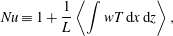 $$\begin{eqnarray}\displaystyle Nu\equiv 1+\frac{1}{L}\left\langle \int wT\,\text{d}x\,\text{d}z\right\rangle , & & \displaystyle\end{eqnarray}$$
where the angle brackets denote a long-time average; i.e. for some function
 $f$
,
$f$
,
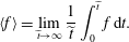 $$\begin{eqnarray}\displaystyle \langle f\rangle =\lim _{\widetilde{t}\rightarrow \infty }\frac{1}{\widetilde{t}}\int _{0}^{\widetilde{t}}f\,\text{d}t. & & \displaystyle\end{eqnarray}$$
From the equations of motion an alternative but equivalent expression for the Nusselt number can be derived (Doering & Constantin Reference Doering and Constantin1998),
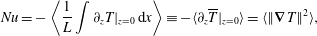 $$\begin{eqnarray}\displaystyle Nu=-\left\langle \frac{1}{L}\int \unicode[STIX]{x2202}_{z}T|_{z=0}\,\text{d}x\right\rangle \equiv -\langle \unicode[STIX]{x2202}_{z}\overline{T}|_{z=0}\rangle =\langle \Vert \unicode[STIX]{x1D735}T\Vert ^{2}\rangle , & & \displaystyle\end{eqnarray}$$
where
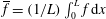 $\overline{f}=(1/L)\int _{0}^{L}f\,\text{d}x$
and
$\overline{f}=(1/L)\int _{0}^{L}f\,\text{d}x$
and
 $\Vert f\Vert =((1/L)\int _{0}^{1}\int _{0}^{L}|f|^{2}\,\text{d}x\,\text{d}z)^{1/2}$
.
$\Vert f\Vert =((1/L)\int _{0}^{1}\int _{0}^{L}|f|^{2}\,\text{d}x\,\text{d}z)^{1/2}$
.
Taking the curl of (2.2) yields the vorticity equation,
 $$\begin{eqnarray}\displaystyle \unicode[STIX]{x1D6FA}=-Ra(\unicode[STIX]{x2202}_{z}T\sin \unicode[STIX]{x1D719}-\unicode[STIX]{x2202}_{x}T\cos \unicode[STIX]{x1D719}), & & \displaystyle\end{eqnarray}$$
where the (negative) scalar vorticity
 $\unicode[STIX]{x1D6FA}=\unicode[STIX]{x2202}_{x}w-\unicode[STIX]{x2202}_{z}u$
. To solve these equations numerically, it is convenient to first introduce a stream function
$\unicode[STIX]{x1D6FA}=\unicode[STIX]{x2202}_{x}w-\unicode[STIX]{x2202}_{z}u$
. To solve these equations numerically, it is convenient to first introduce a stream function
 $\unicode[STIX]{x1D713}$
to describe the fluid motion, so that
$\unicode[STIX]{x1D713}$
to describe the fluid motion, so that
 $(u,w)=(\unicode[STIX]{x2202}_{z}\unicode[STIX]{x1D713},-\unicode[STIX]{x2202}_{x}\unicode[STIX]{x1D713})$
. The dimensionless equations (2.9) and (2.1) then can be expressed as
$(u,w)=(\unicode[STIX]{x2202}_{z}\unicode[STIX]{x1D713},-\unicode[STIX]{x2202}_{x}\unicode[STIX]{x1D713})$
. The dimensionless equations (2.9) and (2.1) then can be expressed as
 $$\begin{eqnarray}\displaystyle & \displaystyle \unicode[STIX]{x1D6FB}^{2}\unicode[STIX]{x1D713}=Ra(\unicode[STIX]{x2202}_{z}\unicode[STIX]{x1D703}\sin \unicode[STIX]{x1D719}-\sin \unicode[STIX]{x1D719}-\unicode[STIX]{x2202}_{x}\unicode[STIX]{x1D703}\cos \unicode[STIX]{x1D719}), & \displaystyle\end{eqnarray}$$
 $$\begin{eqnarray}\displaystyle & \displaystyle \unicode[STIX]{x2202}_{t}\unicode[STIX]{x1D703}+\unicode[STIX]{x2202}_{z}\unicode[STIX]{x1D713}\unicode[STIX]{x2202}_{x}\unicode[STIX]{x1D703}-\unicode[STIX]{x2202}_{x}\unicode[STIX]{x1D713}\unicode[STIX]{x2202}_{z}\unicode[STIX]{x1D703}=-\unicode[STIX]{x2202}_{x}\unicode[STIX]{x1D713}+\unicode[STIX]{x1D6FB}^{2}\unicode[STIX]{x1D703}, & \displaystyle\end{eqnarray}$$
where
 $\unicode[STIX]{x1D703}(x,z,t)=T(x,z,t)-(1-z)$
, and
$\unicode[STIX]{x1D703}(x,z,t)=T(x,z,t)-(1-z)$
, and
 $\unicode[STIX]{x1D703}$
and
$\unicode[STIX]{x1D703}$
and
 $\unicode[STIX]{x1D713}$
satisfy
$\unicode[STIX]{x1D713}$
satisfy
 $L$
-periodic boundary conditions in
$L$
-periodic boundary conditions in
 $x$
and homogeneous Dirichlet boundary conditions at
$x$
and homogeneous Dirichlet boundary conditions at
 $z=0,1$
.
$z=0,1$
.
Unlike the horizontal (i.e.
 $\unicode[STIX]{x1D719}=0^{\circ }$
) case, the inclination of the layer will induce a unidirectional shear flow, even in the absence of convection, which strengthens as
$\unicode[STIX]{x1D719}=0^{\circ }$
) case, the inclination of the layer will induce a unidirectional shear flow, even in the absence of convection, which strengthens as
 $\unicode[STIX]{x1D719}$
is increased. The corresponding (structureless) basic-state solution is given by
$\unicode[STIX]{x1D719}$
is increased. The corresponding (structureless) basic-state solution is given by
 $T=1-z$
,
$T=1-z$
,
 $\boldsymbol{u}=Ra\sin \unicode[STIX]{x1D719}(1/2-z)\boldsymbol{e}_{x}$
and
$\boldsymbol{u}=Ra\sin \unicode[STIX]{x1D719}(1/2-z)\boldsymbol{e}_{x}$
and
 $p=(1/2)Ra\sin \unicode[STIX]{x1D719}x+Ra\cos \unicode[STIX]{x1D719}(z-(1/2)z^{2})$
, as shown schematically in figure 2. As demonstrated in the following sections, the basic-state shear flow dramatically impacts the flow structure and heat transport properties as
$p=(1/2)Ra\sin \unicode[STIX]{x1D719}x+Ra\cos \unicode[STIX]{x1D719}(z-(1/2)z^{2})$
, as shown schematically in figure 2. As demonstrated in the following sections, the basic-state shear flow dramatically impacts the flow structure and heat transport properties as
 $\unicode[STIX]{x1D719}$
is increased.
$\unicode[STIX]{x1D719}$
is increased.
3 Stability and variational analyses
In this section, the results of our linear, nonlinear (i.e. energy) and variational upper-bound analyses of inclined PMC are summarised. These analyses complement our DNS of this phenomenon (described in § 4). Specifically, a gap in the threshold inclination angles for linear and energy stability is identified, indicating the possibility for subcritical instability and thereby accounting for the emergence of large-scale travelling-wave convective states observed in the DNS at values of
 $\unicode[STIX]{x1D719}$
for which the non-convective basic state is predicted to be linearly stable. In addition, the upper-bound analysis yields rigorous bounds on the maximum realisable heat flux in PMC, which cannot, of course, be established through DNS. Nevertheless, it is gratifying that the heat-flux bounds and the heat flux computed via our DNS are found to be in relatively close quantitative agreement.
$\unicode[STIX]{x1D719}$
for which the non-convective basic state is predicted to be linearly stable. In addition, the upper-bound analysis yields rigorous bounds on the maximum realisable heat flux in PMC, which cannot, of course, be established through DNS. Nevertheless, it is gratifying that the heat-flux bounds and the heat flux computed via our DNS are found to be in relatively close quantitative agreement.
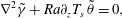
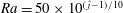
3.1 Linear stability analysis
In their 2D linear stability analysis of inclined PMC, Rees & Bassom (Reference Rees and Bassom2000) focused on the neutral stability of the basic state for
 $Ra\leqslant 1000$
. Here, we revisit the 2D linear stability problem to study the eigenspectrum for disturbances with different wavelengths from the onset of convection up to
$Ra\leqslant 1000$
. Here, we revisit the 2D linear stability problem to study the eigenspectrum for disturbances with different wavelengths from the onset of convection up to
 $Ra=50\,000$
. We also record the asymptotic behaviour of the high-wavenumber branch of marginal modes
$Ra=50\,000$
. We also record the asymptotic behaviour of the high-wavenumber branch of marginal modes
 $k_{l}(Ra)$
and the fastest-growing linear mode
$k_{l}(Ra)$
and the fastest-growing linear mode
 $k_{f}(Ra)$
at large
$k_{f}(Ra)$
at large
 $Ra$
.
$Ra$
.
Setting
 $T=(1-z)+\unicode[STIX]{x1D703}^{\ast }(x,z,t)$
and
$T=(1-z)+\unicode[STIX]{x1D703}^{\ast }(x,z,t)$
and
 $\unicode[STIX]{x1D713}=Ra\sin \unicode[STIX]{x1D719}(z-z^{2})/2+\unicode[STIX]{x1D713}^{\ast }(x,z,t)$
, where
$\unicode[STIX]{x1D713}=Ra\sin \unicode[STIX]{x1D719}(z-z^{2})/2+\unicode[STIX]{x1D713}^{\ast }(x,z,t)$
, where
 $\unicode[STIX]{x1D703}^{\ast }$
and
$\unicode[STIX]{x1D703}^{\ast }$
and
 $\unicode[STIX]{x1D713}^{\ast }$
are small perturbations satisfying periodic boundary conditions in
$\unicode[STIX]{x1D713}^{\ast }$
are small perturbations satisfying periodic boundary conditions in
 $x$
and homogeneous Dirichlet boundary conditions at
$x$
and homogeneous Dirichlet boundary conditions at
 $z=0,1$
, and linearising (2.10)–(2.11) about the basic state yields
$z=0,1$
, and linearising (2.10)–(2.11) about the basic state yields
 $$\begin{eqnarray}\displaystyle & \displaystyle \unicode[STIX]{x1D6FB}^{2}\unicode[STIX]{x1D713}^{\ast }=Ra(\unicode[STIX]{x2202}_{z}\unicode[STIX]{x1D703}^{\ast }\sin \unicode[STIX]{x1D719}-\unicode[STIX]{x2202}_{x}\unicode[STIX]{x1D703}^{\ast }\cos \unicode[STIX]{x1D719}), & \displaystyle\end{eqnarray}$$
 $$\begin{eqnarray}\displaystyle & \displaystyle \unicode[STIX]{x2202}_{t}\unicode[STIX]{x1D703}^{\ast }+{\textstyle \frac{1}{2}}Ra\sin \unicode[STIX]{x1D719}(1-2z)\unicode[STIX]{x2202}_{x}\unicode[STIX]{x1D703}^{\ast }=-\unicode[STIX]{x2202}_{x}\unicode[STIX]{x1D713}^{\ast }+\unicode[STIX]{x1D6FB}^{2}\unicode[STIX]{x1D703}^{\ast }. & \displaystyle\end{eqnarray}$$
The solution of (3.1) and (3.2) for disturbances with wall-parallel wavenumber
 $k$
can be expressed as
$k$
can be expressed as
 $$\begin{eqnarray}\left[\begin{array}{@{}c@{}}\unicode[STIX]{x1D703}^{\ast }\\ \unicode[STIX]{x1D713}^{\ast }\end{array}\right]=\left[\begin{array}{@{}c@{}}\hat{\unicode[STIX]{x1D703}}^{\ast }(z)\\ \hat{\unicode[STIX]{x1D713}}^{\ast }(z)\end{array}\right]\text{e}^{\text{i}kx}\text{e}^{\unicode[STIX]{x1D706}^{\ast }t}+\text{c.c.},\end{eqnarray}$$
where
 $\unicode[STIX]{x1D706}^{\ast }$
is the temporal growth rate and c.c. denotes complex conjugate. Substituting (3.3) into (3.1)–(3.2) yields
$\unicode[STIX]{x1D706}^{\ast }$
is the temporal growth rate and c.c. denotes complex conjugate. Substituting (3.3) into (3.1)–(3.2) yields
 $$\begin{eqnarray}\left[\begin{array}{@{}cc@{}}D_{zz}-k^{2}+\text{i}kRa\sin \unicode[STIX]{x1D719}(z-\frac{1}{2}) & -\text{i}k\\ Ra(\text{i}k\cos \unicode[STIX]{x1D719}-\sin \unicode[STIX]{x1D719}D_{z}) & D_{zz}-k^{2}\end{array}\right]\left[\begin{array}{@{}c@{}}\hat{\unicode[STIX]{x1D703}}^{\ast }\\ \hat{\unicode[STIX]{x1D713}}^{\ast }\end{array}\right]=\unicode[STIX]{x1D706}^{\ast }\left[\begin{array}{@{}cc@{}}I & 0\\ 0 & 0\end{array}\right]\left[\begin{array}{@{}c@{}}\hat{\unicode[STIX]{x1D703}}^{\ast }\\ \hat{\unicode[STIX]{x1D713}}^{\ast }\end{array}\right],\end{eqnarray}$$
where
 $D_{z}$
and
$D_{z}$
and
 $D_{zz}$
denote the first and second partial derivative operators with respect to
$D_{zz}$
denote the first and second partial derivative operators with respect to
 $z$
, respectively, and
$z$
, respectively, and
 $I$
is the identity operator. After discretisation of the
$I$
is the identity operator. After discretisation of the
 $z$
coordinate using a Chebyshev spectral collocation method, we solve (3.4) subject to the boundary conditions
$z$
coordinate using a Chebyshev spectral collocation method, we solve (3.4) subject to the boundary conditions
 $\hat{\unicode[STIX]{x1D703}}^{\ast }=\hat{\unicode[STIX]{x1D713}}^{\ast }=0$
at
$\hat{\unicode[STIX]{x1D703}}^{\ast }=\hat{\unicode[STIX]{x1D713}}^{\ast }=0$
at
 $z=0$
,
$z=0$
,
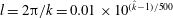
 $1$
using a global generalised eigenvalue routine. Computations are performed for a discrete set of
$1$
using a global generalised eigenvalue routine. Computations are performed for a discrete set of
 $Ra=50\times 10^{(\hat{\jmath }-1)/10}$
from
$Ra=50\times 10^{(\hat{\jmath }-1)/10}$
from
 $Ra=50$
to
$Ra=50$
to
 $Ra=50\,000$
and a discrete set of wall-parallel wavelengths
$Ra=50\,000$
and a discrete set of wall-parallel wavelengths
 $l=2\unicode[STIX]{x03C0}/k=0.01\times 10^{(\hat{k}-1)/500}$
from
$l=2\unicode[STIX]{x03C0}/k=0.01\times 10^{(\hat{k}-1)/500}$
from
 $l=0.01$
to
$l=0.01$
to
 $l=100$
(for integer
$l=100$
(for integer
 $\hat{\jmath }$
and
$\hat{\jmath }$
and
 $\hat{k}$
).
$\hat{k}$
).
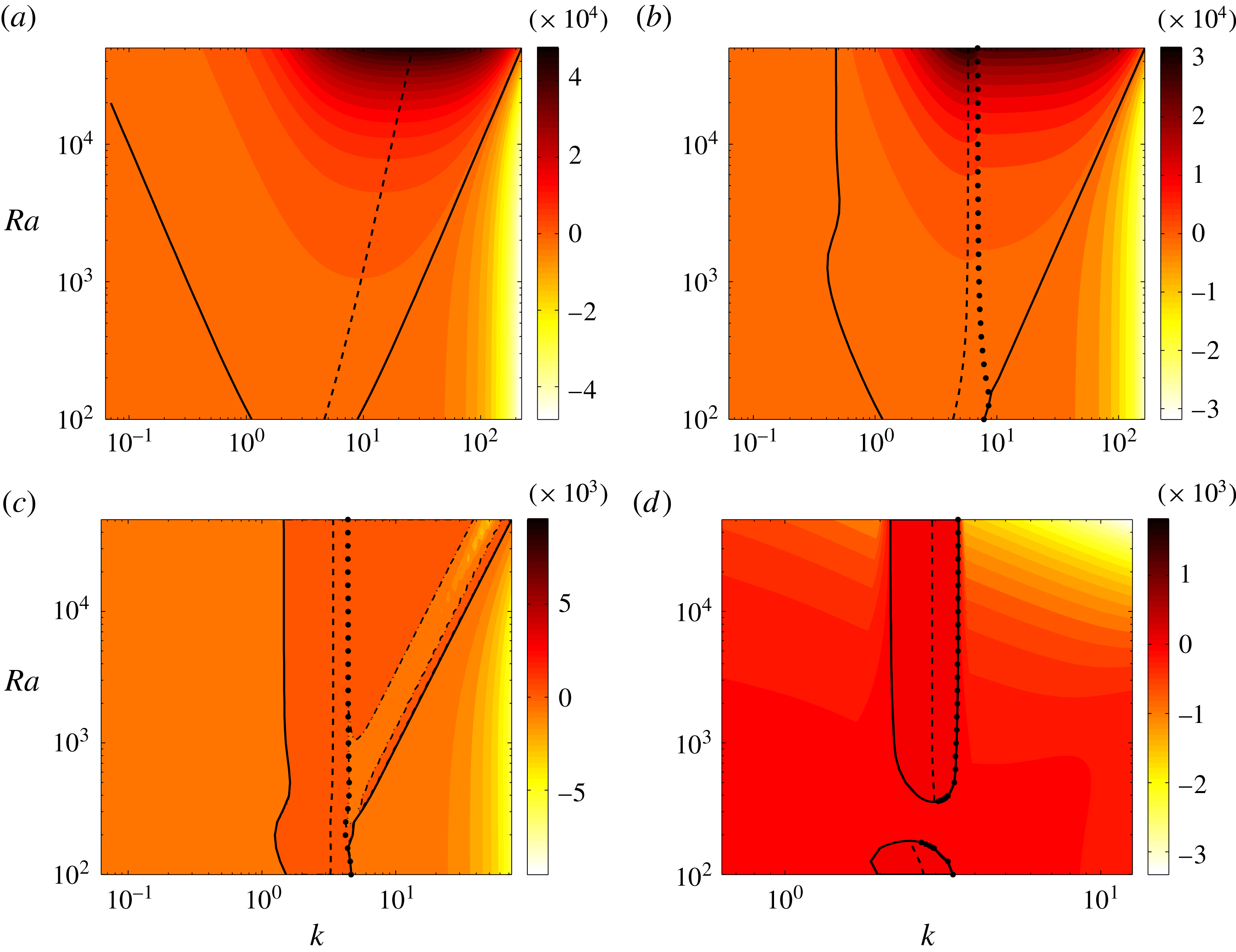
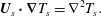
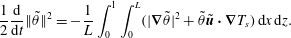
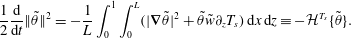
Figure 3. Linear stability results depicted by contour plots of the maximum growth rate
 $\text{Re}\{\unicode[STIX]{x1D706}_{m}^{\ast }\}$
as a function of wavenumber
$\text{Re}\{\unicode[STIX]{x1D706}_{m}^{\ast }\}$
as a function of wavenumber
 $k$
and Rayleigh number
$k$
and Rayleigh number
 $Ra$
: (a)
$Ra$
: (a)
 $\unicode[STIX]{x1D719}=0^{\circ }$
, (b)
$\unicode[STIX]{x1D719}=0^{\circ }$
, (b)
 $\unicode[STIX]{x1D719}=10^{\circ }$
, (c)
$\unicode[STIX]{x1D719}=10^{\circ }$
, (c)
 $\unicode[STIX]{x1D719}=25^{\circ }$
and (d)
$\unicode[STIX]{x1D719}=25^{\circ }$
and (d)
 $\unicode[STIX]{x1D719}=30^{\circ }$
. The solid lines denote the low- and high-wavenumber branches of marginal modes; the dashed line corresponds to the fastest-growing linear mode; and the dotted line separates parameter space into regimes with strictly real (left) and complex (right) eigenvalues. At
$\unicode[STIX]{x1D719}=30^{\circ }$
. The solid lines denote the low- and high-wavenumber branches of marginal modes; the dashed line corresponds to the fastest-growing linear mode; and the dotted line separates parameter space into regimes with strictly real (left) and complex (right) eigenvalues. At
 $\unicode[STIX]{x1D719}=25^{\circ }$
(c), the structure of the growth rate contours is more complicated: the modes between the dotted line and the high-wavenumber branch solid line are not all unstable; e.g. there exists a long narrow band (within the dashed–dotted lines), in which the growth rate is negative. At
$\unicode[STIX]{x1D719}=25^{\circ }$
(c), the structure of the growth rate contours is more complicated: the modes between the dotted line and the high-wavenumber branch solid line are not all unstable; e.g. there exists a long narrow band (within the dashed–dotted lines), in which the growth rate is negative. At
 $\unicode[STIX]{x1D719}=30^{\circ }$
(d), discontinuities in these curves arise because the basic state is linearly stable to all small disturbances for
$\unicode[STIX]{x1D719}=30^{\circ }$
(d), discontinuities in these curves arise because the basic state is linearly stable to all small disturbances for
 $175\lesssim Ra\lesssim 360$
.
$175\lesssim Ra\lesssim 360$
.
Figure 3 shows the contours of maximum growth rate,
 $\text{Re}\{\unicode[STIX]{x1D706}_{m}^{\ast }\}$
(the maximum real part of
$\text{Re}\{\unicode[STIX]{x1D706}_{m}^{\ast }\}$
(the maximum real part of
 $\unicode[STIX]{x1D706}^{\ast }$
), as a function of
$\unicode[STIX]{x1D706}^{\ast }$
), as a function of
 $k$
and
$k$
and
 $Ra$
for various
$Ra$
for various
 $\unicode[STIX]{x1D719}$
. At
$\unicode[STIX]{x1D719}$
. At
 $\unicode[STIX]{x1D719}=0^{\circ }$
, the analytical solution of (3.4) was recorded by Horton & Rogers (Reference Horton and Rogers1945) and Lapwood (Reference Lapwood1948); namely,
$\unicode[STIX]{x1D719}=0^{\circ }$
, the analytical solution of (3.4) was recorded by Horton & Rogers (Reference Horton and Rogers1945) and Lapwood (Reference Lapwood1948); namely,
 $$\begin{eqnarray}\displaystyle \unicode[STIX]{x1D706}^{\ast }=\frac{Ra\,k^{2}}{(m\unicode[STIX]{x03C0})^{2}+k^{2}}-[(m\unicode[STIX]{x03C0})^{2}+k^{2}],\quad \unicode[STIX]{x1D703}^{\ast }=\cos (kx)\sin (m\unicode[STIX]{x03C0}z)\text{e}^{\unicode[STIX]{x1D706}^{\ast }t}, & & \displaystyle\end{eqnarray}$$
where
 $m$
is the integer wall-normal mode number. As evident in (3.5a,b
), all the eigenvalues are strictly real. Moreover, when
$m$
is the integer wall-normal mode number. As evident in (3.5a,b
), all the eigenvalues are strictly real. Moreover, when
 $\unicode[STIX]{x1D719}=0^{\circ }$
and as
$\unicode[STIX]{x1D719}=0^{\circ }$
and as
 $Ra\rightarrow \infty$
, the high-wavenumber branch of marginal modes
$Ra\rightarrow \infty$
, the high-wavenumber branch of marginal modes
 $k_{l}\sim Ra^{1/2}$
and the wavenumber of the fastest-growing linear mode
$k_{l}\sim Ra^{1/2}$
and the wavenumber of the fastest-growing linear mode
 $k_{f}\sim \sqrt{\unicode[STIX]{x03C0}}Ra^{1/4}$
(also see figure 3
a). However, in the inclined case (
$k_{f}\sim \sqrt{\unicode[STIX]{x03C0}}Ra^{1/4}$
(also see figure 3
a). However, in the inclined case (
 $0^{\circ }<\unicode[STIX]{x1D719}<90^{\circ }$
), the linear operator on the left-hand side of (3.4) is no longer self-adjoint and may yield complex eigenvalues. In figure 3(b–d), the unstable eigenvalues (with positive
$0^{\circ }<\unicode[STIX]{x1D719}<90^{\circ }$
), the linear operator on the left-hand side of (3.4) is no longer self-adjoint and may yield complex eigenvalues. In figure 3(b–d), the unstable eigenvalues (with positive
 $\text{Re}\{\unicode[STIX]{x1D706}_{m}^{\ast }\}$
) between the left solid line (corresponding to the low-wavenumber branch of marginal modes) and the dotted line are real, and become complex between the dotted line and the right solid line (corresponding to the high-wavenumber branch of marginal modes). For
$\text{Re}\{\unicode[STIX]{x1D706}_{m}^{\ast }\}$
) between the left solid line (corresponding to the low-wavenumber branch of marginal modes) and the dotted line are real, and become complex between the dotted line and the right solid line (corresponding to the high-wavenumber branch of marginal modes). For
 $0^{\circ }\leqslant \unicode[STIX]{x1D719}\leqslant 25^{\circ }$
,
$0^{\circ }\leqslant \unicode[STIX]{x1D719}\leqslant 25^{\circ }$
,
 $k_{l}\sim C_{l}Ra^{1/2}$
in the high-
$k_{l}\sim C_{l}Ra^{1/2}$
in the high-
 $Ra$
regime, albeit with a
$Ra$
regime, albeit with a
 $\unicode[STIX]{x1D719}$
-dependent prefactor
$\unicode[STIX]{x1D719}$
-dependent prefactor
 $C_{l}$
. The wavenumber of the fastest-growing linear mode in inclined PMC, however, asymptotes to a constant at large values of the Rayleigh number. Furthermore, as
$C_{l}$
. The wavenumber of the fastest-growing linear mode in inclined PMC, however, asymptotes to a constant at large values of the Rayleigh number. Furthermore, as
 $\unicode[STIX]{x1D719}$
is increased, the unstable region (between the two solid lines in figure 3) shrinks and ultimately disappears when
$\unicode[STIX]{x1D719}$
is increased, the unstable region (between the two solid lines in figure 3) shrinks and ultimately disappears when
 $\unicode[STIX]{x1D719}>\unicode[STIX]{x1D719}_{t}$
(note, from the linear stability analysis of Rees & Bassom (Reference Rees and Bassom2000), that
$\unicode[STIX]{x1D719}>\unicode[STIX]{x1D719}_{t}$
(note, from the linear stability analysis of Rees & Bassom (Reference Rees and Bassom2000), that
 $\unicode[STIX]{x1D719}_{t}\approx 31.30^{\circ }$
at large
$\unicode[STIX]{x1D719}_{t}\approx 31.30^{\circ }$
at large
 $Ra$
), implying that the basic state is linearly stable to 2D disturbances at sufficiently large inclination angle.
$Ra$
), implying that the basic state is linearly stable to 2D disturbances at sufficiently large inclination angle.
3.2 Nonlinear energy stability analysis
The linear stability of the thermally stratified base shear flow at sufficiently large
 $\unicode[STIX]{x1D719}$
does not, of course, imply that this basic state is stable to finite-amplitude disturbances. In this section, we employ nonlinear energy stability theory (Doering & Constantin Reference Doering and Constantin1998) to analyse the stability of the basic state to arbitrarily large perturbations as a function of the inclination angle. Consider a 2D steady solution
$\unicode[STIX]{x1D719}$
does not, of course, imply that this basic state is stable to finite-amplitude disturbances. In this section, we employ nonlinear energy stability theory (Doering & Constantin Reference Doering and Constantin1998) to analyse the stability of the basic state to arbitrarily large perturbations as a function of the inclination angle. Consider a 2D steady solution
 $T_{s}(x,z)$
,
$T_{s}(x,z)$
,
 $\boldsymbol{U}_{s}(x,z)$
and
$\boldsymbol{U}_{s}(x,z)$
and
 $P_{s}(x,z)$
(for temperature, velocity and pressure, respectively) to the system
$P_{s}(x,z)$
(for temperature, velocity and pressure, respectively) to the system
 $$\begin{eqnarray}\displaystyle & \displaystyle \unicode[STIX]{x1D735}\boldsymbol{\cdot }\boldsymbol{U}_{s}=0, & \displaystyle\end{eqnarray}$$
 $$\begin{eqnarray}\displaystyle & \displaystyle \boldsymbol{U}_{s}+\unicode[STIX]{x1D735}P_{s}=RaT_{s}\left(\sin \unicode[STIX]{x1D719}\boldsymbol{e}_{x}+\cos \unicode[STIX]{x1D719}\boldsymbol{e}_{z}\right), & \displaystyle\end{eqnarray}$$
 $$\begin{eqnarray}\displaystyle & \displaystyle \boldsymbol{U}_{s}\boldsymbol{\cdot }\unicode[STIX]{x1D735}T_{s}=\unicode[STIX]{x1D6FB}^{2}T_{s}. & \displaystyle\end{eqnarray}$$
Then the equations governing the evolution of finite-amplitude disturbances
 $\tilde{\unicode[STIX]{x1D703}}(x,z,t)$
,
$\tilde{\unicode[STIX]{x1D703}}(x,z,t)$
,
 $\tilde{\boldsymbol{u}}(x,z,t)=\tilde{u} (x,z,t)\boldsymbol{e}_{x}+\tilde{w}(x,z,t)\boldsymbol{e}_{z}$
and
$\tilde{\boldsymbol{u}}(x,z,t)=\tilde{u} (x,z,t)\boldsymbol{e}_{x}+\tilde{w}(x,z,t)\boldsymbol{e}_{z}$
and
 $\tilde{p}(x,z,t)$
to this steady state are
$\tilde{p}(x,z,t)$
to this steady state are
 $$\begin{eqnarray}\displaystyle & \displaystyle \unicode[STIX]{x1D735}\boldsymbol{\cdot }\tilde{\boldsymbol{u}}=0, & \displaystyle\end{eqnarray}$$
 $$\begin{eqnarray}\displaystyle & \displaystyle \tilde{\boldsymbol{u}}+\unicode[STIX]{x1D735}\tilde{p}=Ra\tilde{\unicode[STIX]{x1D703}}\left(\sin \unicode[STIX]{x1D719}\boldsymbol{e}_{x}+\cos \unicode[STIX]{x1D719}\boldsymbol{e}_{z}\right), & \displaystyle\end{eqnarray}$$
 $$\begin{eqnarray}\displaystyle & \displaystyle \tilde{\unicode[STIX]{x1D703}}_{t}+\tilde{\boldsymbol{u}}\boldsymbol{\cdot }\unicode[STIX]{x1D735}\tilde{\unicode[STIX]{x1D703}}+\boldsymbol{U}_{s}\boldsymbol{\cdot }\unicode[STIX]{x1D735}\tilde{\unicode[STIX]{x1D703}}+\tilde{\boldsymbol{u}}\boldsymbol{\cdot }\unicode[STIX]{x1D735}T_{s}=\unicode[STIX]{x1D6FB}^{2}\tilde{\unicode[STIX]{x1D703}}. & \displaystyle\end{eqnarray}$$
The disturbance fields
 $\tilde{\unicode[STIX]{x1D703}}(x,z,t)$
and
$\tilde{\unicode[STIX]{x1D703}}(x,z,t)$
and
 $\tilde{w}(x,z,t)$
satisfy homogeneous Dirichlet boundary conditions at
$\tilde{w}(x,z,t)$
satisfy homogeneous Dirichlet boundary conditions at
 $z=0,1$
and a periodicity condition in
$z=0,1$
and a periodicity condition in
 $x$
. Multiplying equation (3.11) by
$x$
. Multiplying equation (3.11) by
 $\tilde{\unicode[STIX]{x1D703}}$
and integrating over the domain yields an expression for the evolution of the perturbation ‘energy’:
$\tilde{\unicode[STIX]{x1D703}}$
and integrating over the domain yields an expression for the evolution of the perturbation ‘energy’:
 $$\begin{eqnarray}\frac{1}{2}\frac{\text{d}}{\text{d}t}\Vert \tilde{\unicode[STIX]{x1D703}}\Vert ^{2}=-\frac{1}{L}\int _{0}^{1}\int _{0}^{L}(|\unicode[STIX]{x1D735}\tilde{\unicode[STIX]{x1D703}}|^{2}+\tilde{\unicode[STIX]{x1D703}}\tilde{\boldsymbol{u}}\boldsymbol{\cdot }\unicode[STIX]{x1D735}T_{s})\,\text{d}x\,\text{d}z.\end{eqnarray}$$
For any one-dimensional (1D) steady solution
 $T_{s}=T_{s}(z)$
, (3.12) becomes
$T_{s}=T_{s}(z)$
, (3.12) becomes
 $$\begin{eqnarray}\frac{1}{2}\frac{\text{d}}{\text{d}t}\Vert \tilde{\unicode[STIX]{x1D703}}\Vert ^{2}=-\frac{1}{L}\int _{0}^{1}\int _{0}^{L}(|\unicode[STIX]{x1D735}\tilde{\unicode[STIX]{x1D703}}|^{2}+\tilde{\unicode[STIX]{x1D703}}\tilde{w}\unicode[STIX]{x2202}_{z}T_{s})\,\text{d}x\,\text{d}z\equiv -{\mathcal{H}}^{T_{s}}\{\tilde{\unicode[STIX]{x1D703}}\}.\end{eqnarray}$$
As long as the right-hand side of (3.13) is negative (i.e.
 ${\mathcal{H}}^{T_{s}}\geqslant 0$
), arbitrarily large perturbations of the base state will vanish as
${\mathcal{H}}^{T_{s}}\geqslant 0$
), arbitrarily large perturbations of the base state will vanish as
 $t\rightarrow \infty$
. Since
$t\rightarrow \infty$
. Since
 $\tilde{w}$
is a linear non-local functional of
$\tilde{w}$
is a linear non-local functional of
 $\tilde{\unicode[STIX]{x1D703}}$
,
$\tilde{\unicode[STIX]{x1D703}}$
,
 ${\mathcal{H}}^{T_{s}}$
is a quadratic form in terms of
${\mathcal{H}}^{T_{s}}$
is a quadratic form in terms of
 $\tilde{\unicode[STIX]{x1D703}}$
. The positivity constraint for this quadratic form is equivalent to a spectral constraint for the self-adjoint operator inside
$\tilde{\unicode[STIX]{x1D703}}$
. The positivity constraint for this quadratic form is equivalent to a spectral constraint for the self-adjoint operator inside
 ${\mathcal{H}}^{T_{s}}$
: namely, the non-positivity of the ground state eigenvalue
${\mathcal{H}}^{T_{s}}$
: namely, the non-positivity of the ground state eigenvalue
 $\tilde{\unicode[STIX]{x1D706}}^{0}$
of the self-adjoint problem
$\tilde{\unicode[STIX]{x1D706}}^{0}$
of the self-adjoint problem
 $$\begin{eqnarray}\displaystyle & \displaystyle 2\unicode[STIX]{x1D6FB}^{2}\tilde{\unicode[STIX]{x1D703}}-\unicode[STIX]{x2202}_{z}T_{s}\,\tilde{w}+(\cos \unicode[STIX]{x1D719}\unicode[STIX]{x2202}_{x}^{2}\tilde{\unicode[STIX]{x1D6FE}}-\sin \unicode[STIX]{x1D719}\unicode[STIX]{x2202}_{xz}\tilde{\unicode[STIX]{x1D6FE}})=\tilde{\unicode[STIX]{x1D706}}\tilde{\unicode[STIX]{x1D703}}, & \displaystyle\end{eqnarray}$$
 $$\begin{eqnarray}\displaystyle & \displaystyle \unicode[STIX]{x1D6FB}^{2}\tilde{w}-Ra(\cos \unicode[STIX]{x1D719}\unicode[STIX]{x2202}_{x}^{2}\tilde{\unicode[STIX]{x1D703}}-\sin \unicode[STIX]{x1D719}\unicode[STIX]{x2202}_{xz}\tilde{\unicode[STIX]{x1D703}})=0, & \displaystyle\end{eqnarray}$$
 $$\begin{eqnarray}\displaystyle & \displaystyle \unicode[STIX]{x1D6FB}^{2}\tilde{\unicode[STIX]{x1D6FE}}+Ra\unicode[STIX]{x2202}_{z}T_{s}\,\tilde{\unicode[STIX]{x1D703}}=0, & \displaystyle\end{eqnarray}$$
where
 $\tilde{\unicode[STIX]{x1D6FE}}(x,z)$
is the Lagrange-multiplier field enforcing the local constraint (3.15), which can be obtained from (2.3) and (2.9), and (with a slight abuse of notation) the now time-independent
$\tilde{\unicode[STIX]{x1D6FE}}(x,z)$
is the Lagrange-multiplier field enforcing the local constraint (3.15), which can be obtained from (2.3) and (2.9), and (with a slight abuse of notation) the now time-independent
 $\tilde{\unicode[STIX]{x1D703}}(x,z)$
,
$\tilde{\unicode[STIX]{x1D703}}(x,z)$
,
 $\tilde{w}(x,z)$
and
$\tilde{w}(x,z)$
and
 $\tilde{\unicode[STIX]{x1D6FE}}(x,z)$
are eigenfunctions of the system (3.14)–(3.16). Therefore, in the energy stability formulation the spectral constraint
$\tilde{\unicode[STIX]{x1D6FE}}(x,z)$
are eigenfunctions of the system (3.14)–(3.16). Therefore, in the energy stability formulation the spectral constraint
 $\tilde{\unicode[STIX]{x1D706}}^{0}\leqslant 0$
ensures that the steady solution
$\tilde{\unicode[STIX]{x1D706}}^{0}\leqslant 0$
ensures that the steady solution
 $T_{s}(z)$
is energy stable for any perturbation
$T_{s}(z)$
is energy stable for any perturbation
 $\tilde{\unicode[STIX]{x1D703}}(x,z)$
at the given
$\tilde{\unicode[STIX]{x1D703}}(x,z)$
at the given
 $Ra$
.
$Ra$
.
In this section, we set
 $T_{s}=1-z$
(requiring
$T_{s}=1-z$
(requiring
 $U_{s}=Ra(1/2-z)\sin \unicode[STIX]{x1D719}$
) and numerically solve the eigenvalue problem (3.14)–(3.16) using a Chebyshev spectral collocation method to determine, for each
$U_{s}=Ra(1/2-z)\sin \unicode[STIX]{x1D719}$
) and numerically solve the eigenvalue problem (3.14)–(3.16) using a Chebyshev spectral collocation method to determine, for each
 $Ra$
, the inclination angle above which the basic state is energy stable and, for each
$Ra$
, the inclination angle above which the basic state is energy stable and, for each
 $\unicode[STIX]{x1D719}$
, the variation with
$\unicode[STIX]{x1D719}$
, the variation with
 $Ra$
of the wavenumber of the associated marginal energy stable mode
$Ra$
of the wavenumber of the associated marginal energy stable mode
 $k_{e}$
. To meet the first objective, the eigensystem (3.14)–(3.16) was solved for a discrete set of
$k_{e}$
. To meet the first objective, the eigensystem (3.14)–(3.16) was solved for a discrete set of
 $Ra$
,
$Ra$
,
 $\unicode[STIX]{x1D719}$
and
$\unicode[STIX]{x1D719}$
and
 $k$
ranging from
$k$
ranging from
 $Ra=40$
,
$Ra=40$
,
 $\unicode[STIX]{x1D719}=0^{\circ }$
and
$\unicode[STIX]{x1D719}=0^{\circ }$
and
 $k=0$
to
$k=0$
to
 $Ra=200$
,
$Ra=200$
,
 $\unicode[STIX]{x1D719}=90^{\circ }$
and
$\unicode[STIX]{x1D719}=90^{\circ }$
and
 $k=5\unicode[STIX]{x03C0}$
with uniform increments
$k=5\unicode[STIX]{x03C0}$
with uniform increments
 $\unicode[STIX]{x0394}Ra=1$
,
$\unicode[STIX]{x0394}Ra=1$
,
 $\unicode[STIX]{x0394}\unicode[STIX]{x1D719}=0.25^{\circ }$
and
$\unicode[STIX]{x0394}\unicode[STIX]{x1D719}=0.25^{\circ }$
and
 $\unicode[STIX]{x0394}k=0.02\unicode[STIX]{x03C0}$
; for the second, the eigenproblem was solved for a discrete set of
$\unicode[STIX]{x0394}k=0.02\unicode[STIX]{x03C0}$
; for the second, the eigenproblem was solved for a discrete set of
 $Ra=50\times 10^{(\hat{\jmath }-1)/10}$
from
$Ra=50\times 10^{(\hat{\jmath }-1)/10}$
from
 $Ra=50$
to
$Ra=50$
to
 $Ra=125594$
and different wavelengths
$Ra=125594$
and different wavelengths
 $l=2\unicode[STIX]{x03C0}/k=0.01\times 10^{(\hat{k}-1)/500}$
from
$l=2\unicode[STIX]{x03C0}/k=0.01\times 10^{(\hat{k}-1)/500}$
from
 $l=0.01$
to
$l=0.01$
to
 $l=10$
(for integer
$l=10$
(for integer
 $\hat{\jmath }$
and
$\hat{\jmath }$
and
 $\hat{k}$
).
$\hat{k}$
).
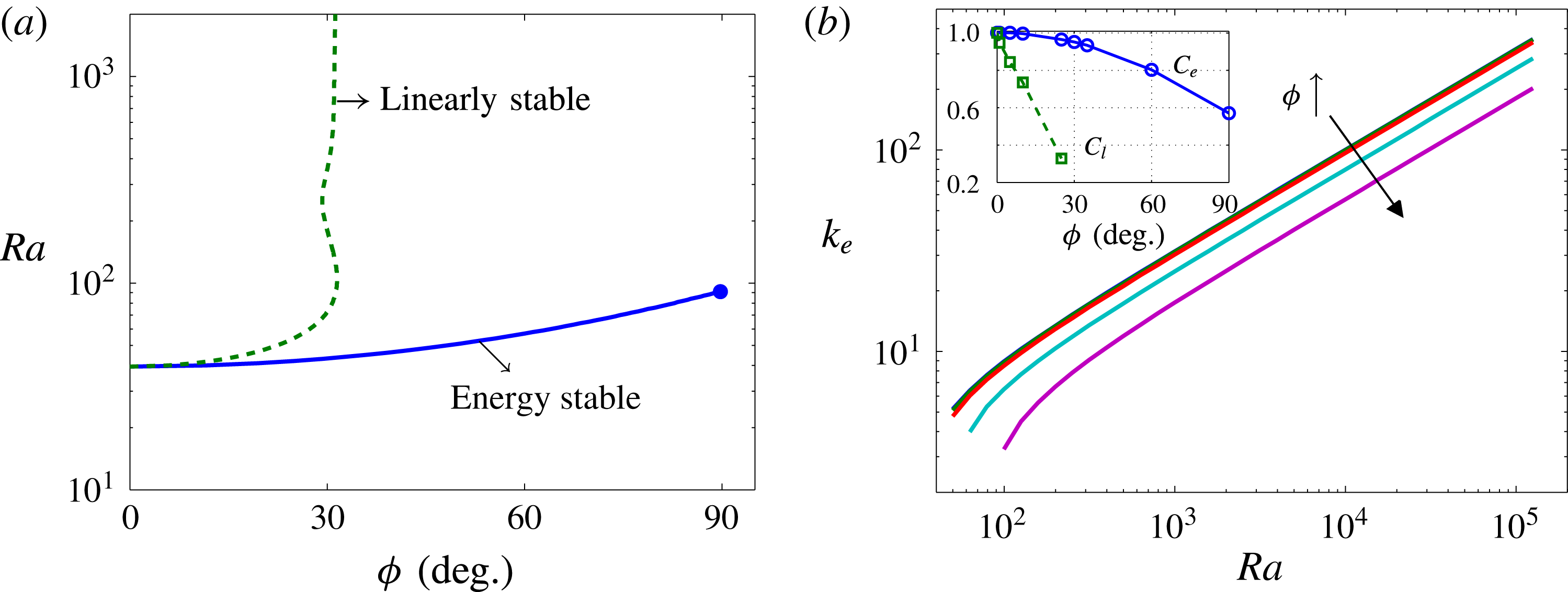
Figure 4. (a) Energy stability (solid curve) and linear stability (dashed curve) boundaries of the basic state
 $T_{s}=1-z$
,
$T_{s}=1-z$
,
 $U_{s}=Ra(1/2-z)\text{sin}\unicode[STIX]{x1D719}$
in the (
$U_{s}=Ra(1/2-z)\text{sin}\unicode[STIX]{x1D719}$
in the (
 $\unicode[STIX]{x1D719},Ra$
)-parameter space for perturbations with arbitrary horizontal wavelengths. At points below and to the right of the solid/dashed curve, the basic state is energy/linearly stable, respectively. At small
$\unicode[STIX]{x1D719},Ra$
)-parameter space for perturbations with arbitrary horizontal wavelengths. At points below and to the right of the solid/dashed curve, the basic state is energy/linearly stable, respectively. At small
 $Ra$
, the basic state is energy/linearly stable for all perturbations above a certain inclination angle. This transition angle for linear stability becomes
$Ra$
, the basic state is energy/linearly stable for all perturbations above a certain inclination angle. This transition angle for linear stability becomes
 $Ra$
-independent at large Rayleigh number:
$Ra$
-independent at large Rayleigh number:
 $\unicode[STIX]{x1D719}_{t}\sim 31.30^{\circ }$
. However, the basic state is not energy stable for any
$\unicode[STIX]{x1D719}_{t}\sim 31.30^{\circ }$
. However, the basic state is not energy stable for any
 $\unicode[STIX]{x1D719}$
when
$\unicode[STIX]{x1D719}$
when
 $Ra\gtrsim 91.6$
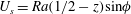
. (b) Variation of the wavenumber
$Ra\gtrsim 91.6$
. (b) Variation of the wavenumber
 $k_{e}$
of the marginal energy stable mode as a function of
$k_{e}$
of the marginal energy stable mode as a function of
 $Ra$
for
$Ra$
for
 $\unicode[STIX]{x1D719}=0^{\circ }$
,
$\unicode[STIX]{x1D719}=0^{\circ }$
,
 $10^{\circ }$
,
$10^{\circ }$
,
 $25^{\circ }$
,
$25^{\circ }$
,
 $60^{\circ }$
and
$60^{\circ }$
and
 $90^{\circ }$
. For
$90^{\circ }$
. For
 $L\leqslant 2\unicode[STIX]{x03C0}/k_{e}$
, the basic state is energy stable. At large
$L\leqslant 2\unicode[STIX]{x03C0}/k_{e}$
, the basic state is energy stable. At large
 $Ra$
,
$Ra$
,
 $k_{e}\sim C_{e}Ra^{1/2}$
, as for the high-wavenumber branch of marginal linear stability modes. The inset shows the variation of the prefactors
$k_{e}\sim C_{e}Ra^{1/2}$
, as for the high-wavenumber branch of marginal linear stability modes. The inset shows the variation of the prefactors
 $C_{l}$
and
$C_{l}$
and
 $C_{e}$
for the linear stability (dashed-square) and energy stability (solid-circle) results, respectively.
$C_{e}$
for the linear stability (dashed-square) and energy stability (solid-circle) results, respectively.
Figure 4(a) shows the energy stability and linear stability boundaries computed over all wavenumbers. Clearly, there exist transition angles for both energy stability and linear stability above which the basic state is energy stable and linearly stable, respectively, at each
 $Ra$
. Of course, if the base state is energy stable, it must be linearly stable. Linearly stable states, however, are not necessarily energy stable, as evident in figure 4(a): at small
$Ra$
. Of course, if the base state is energy stable, it must be linearly stable. Linearly stable states, however, are not necessarily energy stable, as evident in figure 4(a): at small
 $Ra$
, the transition angle for energy stability is much larger than that for linear stability, and for
$Ra$
, the transition angle for energy stability is much larger than that for linear stability, and for
 $0^{\circ }\leqslant \unicode[STIX]{x1D719}\leqslant 90^{\circ }$
, the basic state is not energy stable over all wavenumbers when
$0^{\circ }\leqslant \unicode[STIX]{x1D719}\leqslant 90^{\circ }$
, the basic state is not energy stable over all wavenumbers when
 $Ra\gtrsim 91.6$
; at large
$Ra\gtrsim 91.6$
; at large
 $Ra$
, the transition angle for the linear stability analysis converges to a fixed value independent of
$Ra$
, the transition angle for the linear stability analysis converges to a fixed value independent of
 $Ra$
, i.e.
$Ra$
, i.e.
 $\unicode[STIX]{x1D719}_{t}\sim 31.30^{\circ }$
, as reported in Rees & Bassom (Reference Rees and Bassom2000). The gap in
$\unicode[STIX]{x1D719}_{t}\sim 31.30^{\circ }$
, as reported in Rees & Bassom (Reference Rees and Bassom2000). The gap in
 $\unicode[STIX]{x1D719}$
(at fixed
$\unicode[STIX]{x1D719}$
(at fixed
 $Ra$
) between the linear and energy stability thresholds implies the possibility of subcritical instability: as shown in § 4, subcritical instability indeed manifests in inclined PMC in the form of large-scale travelling-wave convective states.
$Ra$
) between the linear and energy stability thresholds implies the possibility of subcritical instability: as shown in § 4, subcritical instability indeed manifests in inclined PMC in the form of large-scale travelling-wave convective states.
Figure 4(b) shows the marginally energy stable wavenumber
 $k_{e}$
as a function of
$k_{e}$
as a function of
 $Ra$
for a range of
$Ra$
for a range of
 $\unicode[STIX]{x1D719}$
values. As for the high-wavenumber marginal linear stability mode (for
$\unicode[STIX]{x1D719}$
values. As for the high-wavenumber marginal linear stability mode (for
 $\unicode[STIX]{x1D719}<30^{\circ }$
, see figure 3), the wavenumber of the marginal energy stability mode
$\unicode[STIX]{x1D719}<30^{\circ }$
, see figure 3), the wavenumber of the marginal energy stability mode
 $k_{e}\sim C_{e}Ra^{1/2}$
for
$k_{e}\sim C_{e}Ra^{1/2}$
for
 $0^{\circ }\leqslant \unicode[STIX]{x1D719}\leqslant 90^{\circ }$
at large Rayleigh number, with a prefactor
$0^{\circ }\leqslant \unicode[STIX]{x1D719}\leqslant 90^{\circ }$
at large Rayleigh number, with a prefactor
 $C_{e}$
that decreases as
$C_{e}$
that decreases as
 $\unicode[STIX]{x1D719}$
is increased; that is, for fixed
$\unicode[STIX]{x1D719}$
is increased; that is, for fixed
 $Ra$
, the (energy) marginal wavelength increases as
$Ra$
, the (energy) marginal wavelength increases as
 $\unicode[STIX]{x1D719}$
is increased. This large-
$\unicode[STIX]{x1D719}$
is increased. This large-
 $Ra$
wavenumber scaling of the marginal energy stability mode is compared later in § 4, figure 8 with the mean wavenumber scaling exhibited in spatiotemporally chaotic PMC as extracted from our DNS.
$Ra$
wavenumber scaling of the marginal energy stability mode is compared later in § 4, figure 8 with the mean wavenumber scaling exhibited in spatiotemporally chaotic PMC as extracted from our DNS.
3.3 Variational upper-bound analysis
Previous studies by Doering & Constantin (Reference Doering and Constantin1998), Otero et al. (Reference Otero, Dontcheva, Johnston, Worthing, Kurganov, Petrova and Doering2004) and Wen et al. (Reference Wen, Chini, Dianati and Doering2013) have shown that the Constantin–Doering–Hopf (CDH) variational upper-bound analysis yields the
 $Nu\sim Ra$
scaling observed in high-
$Nu\sim Ra$
scaling observed in high-
 $Ra$
PMC in a horizontal layer. Following these studies, we employ the CDH variational formalism to obtain rigorous bounds on the heat transport in inclined PMC, and provide an interpretation of this formalism using the energy stability theory discussed in § 3.2. We begin by decomposing the temperature
$Ra$
PMC in a horizontal layer. Following these studies, we employ the CDH variational formalism to obtain rigorous bounds on the heat transport in inclined PMC, and provide an interpretation of this formalism using the energy stability theory discussed in § 3.2. We begin by decomposing the temperature
 $T(x,z,t)$
into a time-independent 1D background profile
$T(x,z,t)$
into a time-independent 1D background profile
 $\unicode[STIX]{x1D70F}(z)$
carrying the inhomogeneous boundary conditions plus a nonlinear fluctuation
$\unicode[STIX]{x1D70F}(z)$
carrying the inhomogeneous boundary conditions plus a nonlinear fluctuation
 $\unicode[STIX]{x1D703}(x,z,t)$
satisfying periodic boundary conditions in
$\unicode[STIX]{x1D703}(x,z,t)$
satisfying periodic boundary conditions in
 $x$
and homogeneous Dirichlet boundary conditions in
$x$
and homogeneous Dirichlet boundary conditions in
 $z$
:
$z$
:
 $$\begin{eqnarray}T(x,z,t)=\unicode[STIX]{x1D70F}(z)+\unicode[STIX]{x1D703}(x,z,t),\end{eqnarray}$$
where
 $\unicode[STIX]{x1D70F}(0)=1$
,
$\unicode[STIX]{x1D70F}(0)=1$
,
 $\unicode[STIX]{x1D70F}(1)=0$
and
$\unicode[STIX]{x1D70F}(1)=0$
and
 $\unicode[STIX]{x1D703}(x,0,t)=\unicode[STIX]{x1D703}(x,1,t)=0$
. From the advection–diffusion equation (2.1), the temperature fluctuations
$\unicode[STIX]{x1D703}(x,0,t)=\unicode[STIX]{x1D703}(x,1,t)=0$
. From the advection–diffusion equation (2.1), the temperature fluctuations
 $\unicode[STIX]{x1D703}(x,z,t)$
satisfy
$\unicode[STIX]{x1D703}(x,z,t)$
satisfy
 $$\begin{eqnarray}\unicode[STIX]{x2202}_{t}\unicode[STIX]{x1D703}+\boldsymbol{u}\boldsymbol{\cdot }\unicode[STIX]{x1D735}\unicode[STIX]{x1D703}=-w\unicode[STIX]{x2202}_{z}\unicode[STIX]{x1D70F}+\unicode[STIX]{x1D6FB}^{2}\unicode[STIX]{x1D703}+\unicode[STIX]{x2202}_{z}^{2}\unicode[STIX]{x1D70F}.\end{eqnarray}$$
Multiplying (3.18) by
 $\unicode[STIX]{x1D703}$
and integrating over the domain yields
$\unicode[STIX]{x1D703}$
and integrating over the domain yields
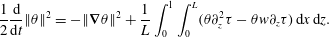 $$\begin{eqnarray}\displaystyle \frac{1}{2}\frac{\text{d}}{\text{d}t}\Vert \unicode[STIX]{x1D703}\Vert ^{2}=-\Vert \unicode[STIX]{x1D735}\unicode[STIX]{x1D703}\Vert ^{2}+\frac{1}{L}\int _{0}^{1}\int _{0}^{L}(\unicode[STIX]{x1D703}\unicode[STIX]{x2202}_{z}^{2}\unicode[STIX]{x1D70F}-\unicode[STIX]{x1D703}w\unicode[STIX]{x2202}_{z}\unicode[STIX]{x1D70F})\,\text{d}x\,\text{d}z. & & \displaystyle\end{eqnarray}$$
Recalling the definition of
 $\Vert \cdot \Vert$
and using (3.17), we have
$\Vert \cdot \Vert$
and using (3.17), we have
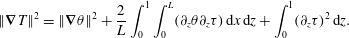 $$\begin{eqnarray}\Vert \unicode[STIX]{x1D735}T\Vert ^{2}=\Vert \unicode[STIX]{x1D735}\unicode[STIX]{x1D703}\Vert ^{2}+\frac{2}{L}\int _{0}^{1}\int _{0}^{L}(\unicode[STIX]{x2202}_{z}\unicode[STIX]{x1D703}\unicode[STIX]{x2202}_{z}\unicode[STIX]{x1D70F})\,\text{d}x\,\text{d}z+\int _{0}^{1}(\unicode[STIX]{x2202}_{z}\unicode[STIX]{x1D70F})^{2}\,\text{d}z.\end{eqnarray}$$
Finally, taking the long-time average of
 $c$
$c$
 $\times$
(3.19)
$\times$
(3.19)
 $+$
(3.20) with
$+$
(3.20) with
 $c>1$
produces
$c>1$
produces
 $$\begin{eqnarray}Nu=\int _{0}^{1}(\unicode[STIX]{x2202}_{z}\unicode[STIX]{x1D70F})^{2}\,\text{d}z-\left\langle \frac{1}{L}\int _{0}^{1}\int _{0}^{L}\left((c-1)|\unicode[STIX]{x1D735}\unicode[STIX]{x1D703}|^{2}+c\unicode[STIX]{x1D703}w\unicode[STIX]{x2202}_{z}\unicode[STIX]{x1D70F}+(2-c)\unicode[STIX]{x1D703}\unicode[STIX]{x2202}_{z}^{2}\unicode[STIX]{x1D70F}\right)\,\text{d}x\,\text{d}z\right\rangle .\end{eqnarray}$$
An upper bound on
 $Nu$
can be obtained by replacing the second term on the right-hand side of (3.21) by its minimum over all relevant
$Nu$
can be obtained by replacing the second term on the right-hand side of (3.21) by its minimum over all relevant
 $\unicode[STIX]{x1D703}(x,z)$
and
$\unicode[STIX]{x1D703}(x,z)$
and
 $w(x,z)$
, namely,
$w(x,z)$
, namely,
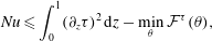 $$\begin{eqnarray}Nu\leqslant \int _{0}^{1}(\unicode[STIX]{x2202}_{z}\unicode[STIX]{x1D70F})^{2}\,\text{d}z-\min _{\unicode[STIX]{x1D703}}{\mathcal{F}}^{\unicode[STIX]{x1D70F}}(\unicode[STIX]{x1D703}),\end{eqnarray}$$
where
 $$\begin{eqnarray}{\mathcal{F}}^{\unicode[STIX]{x1D70F}}(\unicode[STIX]{x1D703})\equiv \frac{1}{L}\int _{0}^{1}\int _{0}^{L}\left((c-1)|\unicode[STIX]{x1D735}\unicode[STIX]{x1D703}|^{2}+c\unicode[STIX]{x1D703}w\unicode[STIX]{x2202}_{z}\unicode[STIX]{x1D70F}+(2-c)\unicode[STIX]{x1D703}\unicode[STIX]{x2202}_{z}^{2}\unicode[STIX]{x1D70F}\right)\,\text{d}x\,\text{d}z.\end{eqnarray}$$
The Euler–Lagrange equations for minimising
 ${\mathcal{F}}^{\unicode[STIX]{x1D70F}}(\unicode[STIX]{x1D703})$
can be obtained by taking the first variations (Frechet derivatives) of the Lagrange functional
${\mathcal{F}}^{\unicode[STIX]{x1D70F}}(\unicode[STIX]{x1D703})$
can be obtained by taking the first variations (Frechet derivatives) of the Lagrange functional
 $$\begin{eqnarray}{\mathcal{L}}^{F}={\mathcal{F}}^{\unicode[STIX]{x1D70F}}(\unicode[STIX]{x1D703})-\frac{1}{L}\int _{0}^{1}\int _{0}^{L}W\left[\unicode[STIX]{x1D6FB}^{2}w-Ra(\cos \unicode[STIX]{x1D719}\unicode[STIX]{x2202}_{x}^{2}\unicode[STIX]{x1D703}-\sin \unicode[STIX]{x1D719}\unicode[STIX]{x2202}_{xz}\unicode[STIX]{x1D703})\right]\,\text{d}x\,\text{d}z,\end{eqnarray}$$
with respect to
 $\unicode[STIX]{x1D703}$
,
$\unicode[STIX]{x1D703}$
,
 $w$
and the Lagrange-multiplier field
$w$
and the Lagrange-multiplier field
 $W$
, which also satisfies periodic boundary conditions in
$W$
, which also satisfies periodic boundary conditions in
 $x$
and homogeneous Dirichlet conditions at
$x$
and homogeneous Dirichlet conditions at
 $z=0,1$
:
$z=0,1$
:
 $$\begin{eqnarray}\displaystyle & \displaystyle -2(c-1)\unicode[STIX]{x1D6FB}^{2}\unicode[STIX]{x1D703}+cw\unicode[STIX]{x2202}_{z}\unicode[STIX]{x1D70F}+Ra(\cos \unicode[STIX]{x1D719}\unicode[STIX]{x2202}_{x}^{2}W-\sin \unicode[STIX]{x1D719}\unicode[STIX]{x2202}_{xz}W)+(2-c)\unicode[STIX]{x2202}_{z}^{2}\unicode[STIX]{x1D70F}=0, & \displaystyle\end{eqnarray}$$
 $$\begin{eqnarray}\displaystyle & \displaystyle \unicode[STIX]{x1D6FB}^{2}w-Ra(\cos \unicode[STIX]{x1D719}\unicode[STIX]{x2202}_{x}^{2}\unicode[STIX]{x1D703}-\sin \unicode[STIX]{x1D719}\unicode[STIX]{x2202}_{xz}\unicode[STIX]{x1D703})=0, & \displaystyle\end{eqnarray}$$
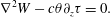 $$\begin{eqnarray}\displaystyle & \displaystyle \unicode[STIX]{x1D6FB}^{2}W-c\unicode[STIX]{x1D703}\unicode[STIX]{x2202}_{z}\unicode[STIX]{x1D70F}=0. & \displaystyle\end{eqnarray}$$
The horizontal mean of (3.25) is
 $$\begin{eqnarray}-2(c-1)\unicode[STIX]{x2202}_{z}^{2}\overline{\unicode[STIX]{x1D703}}+(2-c)\unicode[STIX]{x2202}_{z}^{2}\unicode[STIX]{x1D70F}=0.\end{eqnarray}$$
Integrating twice in
 $z$
yields
$z$
yields
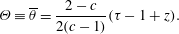 $$\begin{eqnarray}\unicode[STIX]{x1D6E9}\equiv \overline{\unicode[STIX]{x1D703}}=\frac{2-c}{2(c-1)}(\unicode[STIX]{x1D70F}-1+z).\end{eqnarray}$$
Equation (3.29) is a necessary but not sufficient condition to minimise
 ${\mathcal{F}}^{\unicode[STIX]{x1D70F}}$
. Substituting
${\mathcal{F}}^{\unicode[STIX]{x1D70F}}$
. Substituting
 $\unicode[STIX]{x1D703}=\unicode[STIX]{x1D6E9}+\unicode[STIX]{x1D717}$
(where
$\unicode[STIX]{x1D703}=\unicode[STIX]{x1D6E9}+\unicode[STIX]{x1D717}$
(where
 $\overline{\unicode[STIX]{x1D717}}=0$
) into (3.22) and letting
$\overline{\unicode[STIX]{x1D717}}=0$
) into (3.22) and letting
 $a=1-c^{-1}$
(so that
$a=1-c^{-1}$
(so that
 $0<a<1$
) yields
$0<a<1$
) yields
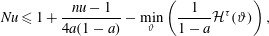 $$\begin{eqnarray}Nu\leqslant 1+\frac{nu-1}{4a(1-a)}-\min _{\unicode[STIX]{x1D717}}\left(\frac{1}{1-a}{\mathcal{H}}^{\unicode[STIX]{x1D70F}}(\unicode[STIX]{x1D717})\right),\end{eqnarray}$$
where
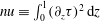 $nu\equiv \int _{0}^{1}(\unicode[STIX]{x2202}_{z}\unicode[STIX]{x1D70F})^{2}\,\text{d}z$
and
$nu\equiv \int _{0}^{1}(\unicode[STIX]{x2202}_{z}\unicode[STIX]{x1D70F})^{2}\,\text{d}z$
and
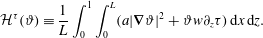 $$\begin{eqnarray}{\mathcal{H}}^{\unicode[STIX]{x1D70F}}(\unicode[STIX]{x1D717})\equiv \frac{1}{L}\int _{0}^{1}\int _{0}^{L}(a|\unicode[STIX]{x1D735}\unicode[STIX]{x1D717}|^{2}+\unicode[STIX]{x1D717}w\unicode[STIX]{x2202}_{z}\unicode[STIX]{x1D70F})\,\text{d}x\,\text{d}z.\end{eqnarray}$$
For any
 $\unicode[STIX]{x1D70F}(z)$
satisfying
$\unicode[STIX]{x1D70F}(z)$
satisfying
 $\unicode[STIX]{x1D70F}(0)=1$
and
$\unicode[STIX]{x1D70F}(0)=1$
and
 $\unicode[STIX]{x1D70F}(1)=0$
and for any
$\unicode[STIX]{x1D70F}(1)=0$
and for any
 $a\in (0,1)$
,
$a\in (0,1)$
,
 $$\begin{eqnarray}\displaystyle Nu\leqslant 1+\frac{nu-1}{4a(1-a)} & & \displaystyle\end{eqnarray}$$
if and only if the spectral constraint
 $$\begin{eqnarray}\displaystyle \min _{\unicode[STIX]{x1D717}}{\mathcal{H}}^{\unicode[STIX]{x1D70F}}(\unicode[STIX]{x1D717})\geqslant 0 & & \displaystyle\end{eqnarray}$$
holds for all test functions
 $\unicode[STIX]{x1D717}(x,z)$
and
$\unicode[STIX]{x1D717}(x,z)$
and
 $w(x,z)$
, where
$w(x,z)$
, where
 $\unicode[STIX]{x1D6FB}^{2}w=Ra(\cos \unicode[STIX]{x1D719}\unicode[STIX]{x2202}_{x}^{2}\unicode[STIX]{x1D717}-\sin \unicode[STIX]{x1D719}\unicode[STIX]{x2202}_{xz}\unicode[STIX]{x1D717})$
, satisfying homogeneous Dirichlet boundary conditions at
$\unicode[STIX]{x1D6FB}^{2}w=Ra(\cos \unicode[STIX]{x1D719}\unicode[STIX]{x2202}_{x}^{2}\unicode[STIX]{x1D717}-\sin \unicode[STIX]{x1D719}\unicode[STIX]{x2202}_{xz}\unicode[STIX]{x1D717})$
, satisfying homogeneous Dirichlet boundary conditions at
 $z=0,1$
and
$z=0,1$
and
 $L$
-periodic boundary conditions in
$L$
-periodic boundary conditions in
 $x$
. It should be noted that compared with those in the horizontal case (Doering & Constantin Reference Doering and Constantin1998; Otero et al.
Reference Otero, Dontcheva, Johnston, Worthing, Kurganov, Petrova and Doering2004), the expressions for the upper bound (3.32) and the spectral constraint (3.33) in the inclined case remain unchanged except that the local constraint (3.26) is more general by allowing for
$x$
. It should be noted that compared with those in the horizontal case (Doering & Constantin Reference Doering and Constantin1998; Otero et al.
Reference Otero, Dontcheva, Johnston, Worthing, Kurganov, Petrova and Doering2004), the expressions for the upper bound (3.32) and the spectral constraint (3.33) in the inclined case remain unchanged except that the local constraint (3.26) is more general by allowing for
 $\unicode[STIX]{x1D719}\neq 0^{\circ }$
.
$\unicode[STIX]{x1D719}\neq 0^{\circ }$
.
For PMC, the balance parameter
 $a$
can be scaled out by defining
$a$
can be scaled out by defining
 $ra=Ra/a$
and
$ra=Ra/a$
and
 $\widetilde{\unicode[STIX]{x1D717}}=a\unicode[STIX]{x1D717}$
, implying
$\widetilde{\unicode[STIX]{x1D717}}=a\unicode[STIX]{x1D717}$
, implying
 $\unicode[STIX]{x1D6FB}^{2}w=ra(\cos \unicode[STIX]{x1D719}\unicode[STIX]{x2202}_{x}^{2}\widetilde{\unicode[STIX]{x1D717}}-\sin \unicode[STIX]{x1D719}\unicode[STIX]{x2202}_{xz}\widetilde{\unicode[STIX]{x1D717}})$
, so that the spectral constraint becomes
$\unicode[STIX]{x1D6FB}^{2}w=ra(\cos \unicode[STIX]{x1D719}\unicode[STIX]{x2202}_{x}^{2}\widetilde{\unicode[STIX]{x1D717}}-\sin \unicode[STIX]{x1D719}\unicode[STIX]{x2202}_{xz}\widetilde{\unicode[STIX]{x1D717}})$
, so that the spectral constraint becomes
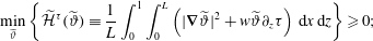 $$\begin{eqnarray}\displaystyle \min _{\widetilde{\unicode[STIX]{x1D717}}}\left\{\widetilde{{\mathcal{H}}}^{\unicode[STIX]{x1D70F}}(\widetilde{\unicode[STIX]{x1D717}})\equiv \frac{1}{L}\int _{0}^{1}\int _{0}^{L}\left(|\unicode[STIX]{x1D735}\widetilde{\unicode[STIX]{x1D717}}|^{2}+w\widetilde{\unicode[STIX]{x1D717}}\unicode[STIX]{x2202}_{z}\unicode[STIX]{x1D70F}\right)\,\text{d}x\,\text{d}z\right\}\geqslant 0; & & \displaystyle\end{eqnarray}$$
i.e. the functional
 $\widetilde{{\mathcal{H}}}^{\unicode[STIX]{x1D70F}}$
must be positive semi-definite for all test functions
$\widetilde{{\mathcal{H}}}^{\unicode[STIX]{x1D70F}}$
must be positive semi-definite for all test functions
 $\widetilde{\unicode[STIX]{x1D717}}(x,z)$
satisfying appropriate boundary conditions. As in § 3.2, the positivity constraint for the quadratic form
$\widetilde{\unicode[STIX]{x1D717}}(x,z)$
satisfying appropriate boundary conditions. As in § 3.2, the positivity constraint for the quadratic form
 $\widetilde{{\mathcal{H}}}^{\unicode[STIX]{x1D70F}}$
is equivalent to a spectral constraint for the self-adjoint operator inside
$\widetilde{{\mathcal{H}}}^{\unicode[STIX]{x1D70F}}$
is equivalent to a spectral constraint for the self-adjoint operator inside
 $\widetilde{{\mathcal{H}}}^{\unicode[STIX]{x1D70F}}$
, namely the non-positivity of the ground state eigenvalue
$\widetilde{{\mathcal{H}}}^{\unicode[STIX]{x1D70F}}$
, namely the non-positivity of the ground state eigenvalue
 $\unicode[STIX]{x1D706}^{0}$
of the self-adjoint problem
$\unicode[STIX]{x1D706}^{0}$
of the self-adjoint problem
 $$\begin{eqnarray}\displaystyle & \displaystyle 2\unicode[STIX]{x1D6FB}^{2}\widetilde{\unicode[STIX]{x1D717}}-\unicode[STIX]{x2202}_{z}\unicode[STIX]{x1D70F}\,w+(\cos \unicode[STIX]{x1D719}\unicode[STIX]{x2202}_{x}^{2}\unicode[STIX]{x1D6FE}-\sin \unicode[STIX]{x1D719}\unicode[STIX]{x2202}_{xz}\unicode[STIX]{x1D6FE})=\unicode[STIX]{x1D706}\widetilde{\unicode[STIX]{x1D717}}, & \displaystyle\end{eqnarray}$$
 $$\begin{eqnarray}\displaystyle & \displaystyle \unicode[STIX]{x1D6FB}^{2}w-ra(\cos \unicode[STIX]{x1D719}\unicode[STIX]{x2202}_{x}^{2}\widetilde{\unicode[STIX]{x1D717}}-\sin \unicode[STIX]{x1D719}\unicode[STIX]{x2202}_{xz}\widetilde{\unicode[STIX]{x1D717}})=0, & \displaystyle\end{eqnarray}$$
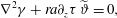 $$\begin{eqnarray}\displaystyle & \displaystyle \unicode[STIX]{x1D6FB}^{2}\unicode[STIX]{x1D6FE}+ra\unicode[STIX]{x2202}_{z}\unicode[STIX]{x1D70F}\,\widetilde{\unicode[STIX]{x1D717}}=0, & \displaystyle\end{eqnarray}$$
where
 $\unicode[STIX]{x1D6FE}(x,z)$
is the Lagrange-multiplier field enforcing the local constraint (3.36). To obtain the optimal upper bound,
$\unicode[STIX]{x1D6FE}(x,z)$
is the Lagrange-multiplier field enforcing the local constraint (3.36). To obtain the optimal upper bound,
 $nu$
is minimised subject to this rescaled spectral constraint
$nu$
is minimised subject to this rescaled spectral constraint
 $\unicode[STIX]{x1D706}^{0}\leqslant 0$
, which is independent of
$\unicode[STIX]{x1D706}^{0}\leqslant 0$
, which is independent of
 $a$
, for a range of
$a$
, for a range of
 $ra$
. Finally, varying
$ra$
. Finally, varying
 $a$
for each
$a$
for each
 $(ra,nu)$
pair produces a family of curves in the
$(ra,nu)$
pair produces a family of curves in the
 $Ra$
–
$Ra$
–
 $Nu$
plane whose lower envelope yields the best bound.
$Nu$
plane whose lower envelope yields the best bound.
In the energy stability formulation, satisfaction of the spectral constraint
 $\tilde{\unicode[STIX]{x1D706}}^{0}\leqslant 0$
ensures that the steady solution
$\tilde{\unicode[STIX]{x1D706}}^{0}\leqslant 0$
ensures that the steady solution
 $T_{s}$
is energy stable for any perturbation
$T_{s}$
is energy stable for any perturbation
 $\tilde{\unicode[STIX]{x1D703}}(x,z)$
at the given
$\tilde{\unicode[STIX]{x1D703}}(x,z)$
at the given
 $Ra$
. In the upper-bound formulation, however, the spectral constraint
$Ra$
. In the upper-bound formulation, however, the spectral constraint
 $\unicode[STIX]{x1D706}^{0}\leqslant 0$
indicates that for any
$\unicode[STIX]{x1D706}^{0}\leqslant 0$
indicates that for any
 $a\in (0,1)$
the right-hand side of (3.32) is a rigorous upper bound on
$a\in (0,1)$
the right-hand side of (3.32) is a rigorous upper bound on
 $Nu$
at the given
$Nu$
at the given
 $Ra$
. Interestingly, comparing (3.35)–(3.37) with (3.14)–(3.16) suggests the following alternative interpretation of the upper-bound spectral constraint:
$Ra$
. Interestingly, comparing (3.35)–(3.37) with (3.14)–(3.16) suggests the following alternative interpretation of the upper-bound spectral constraint:
 $\unicode[STIX]{x1D706}^{0}\leqslant 0$
implies
$\unicode[STIX]{x1D706}^{0}\leqslant 0$
implies
 $\unicode[STIX]{x1D70F}(z)$
is energy stable at
$\unicode[STIX]{x1D70F}(z)$
is energy stable at
 $ra\equiv Ra/a$
as if it were a steady, exact solution. Hence, for
$ra\equiv Ra/a$
as if it were a steady, exact solution. Hence, for
 $a=1$
(i.e.
$a=1$
(i.e.
 $ra=Ra$
), the spectral constraint
$ra=Ra$
), the spectral constraint
 $\unicode[STIX]{x1D706}^{0}\leqslant 0$
requires all fluctuations to the background profile
$\unicode[STIX]{x1D706}^{0}\leqslant 0$
requires all fluctuations to the background profile
 $\unicode[STIX]{x1D70F}(z)$
to be energy stable at the actual value of
$\unicode[STIX]{x1D70F}(z)$
to be energy stable at the actual value of
 $Ra$
as if
$Ra$
as if
 $\unicode[STIX]{x1D70F}(z)$
were a steady solution of the governing equations. Although the right-hand side of (3.32) clearly no longer provides a bound on
$\unicode[STIX]{x1D70F}(z)$
were a steady solution of the governing equations. Although the right-hand side of (3.32) clearly no longer provides a bound on
 $Nu$
for
$Nu$
for
 $a=1$
, this procedure (i.e. minimising the functional
$a=1$
, this procedure (i.e. minimising the functional
 $nu$
subject to
$nu$
subject to
 $\unicode[STIX]{x1D706}^{0}\leqslant 0$
with
$\unicode[STIX]{x1D706}^{0}\leqslant 0$
with
 $a=1$
) nevertheless yields a useful prediction of
$a=1$
) nevertheless yields a useful prediction of
 $Nu$
at the given
$Nu$
at the given
 $Ra$
; indeed, the minimum value of
$Ra$
; indeed, the minimum value of
 $nu$
will be shown to fall below the upper bound, and thus lie even closer to the true heat flux.
$nu$
will be shown to fall below the upper bound, and thus lie even closer to the true heat flux.
The solution (more properly, the global optimal) of the CDH variational problem can be obtained by solving the corresponding Euler–Lagrange equations. In this investigation, the appropriate Euler–Lagrange equations are solved numerically using a time-stepping algorithm developed in Wen et al. (Reference Wen, Chini, Dianati and Doering2013) for the CDH upper-bound problem. Wen et al. (Reference Wen, Chini, Kerswell and Doering2015a ) proved that for Rayleigh–Bénard convection in a horizontal porous layer the steady state reached by the numerical computations reported in Wen et al. (Reference Wen, Chini, Dianati and Doering2013) must be the desired global optimal (or true solution) of the relevant variational problem. Our numerical results suggest that this time-stepping approach also is applicable to the inclined case, although we have not endeavoured to extend the proof.
In this study, the computations were performed for a discrete set of
 $Ra=50\times 10^{(\hat{\jmath }-1)/10}$
from
$Ra=50\times 10^{(\hat{\jmath }-1)/10}$
from
 $Ra=50$
to
$Ra=50$
to
 $Ra=19\,905$
at different inclination angles, as shown in figure 5. Relative to the horizontal case, the inclination of the layer does not affect the unit power-law scaling of the heat-flux prediction (
$Ra=19\,905$
at different inclination angles, as shown in figure 5. Relative to the horizontal case, the inclination of the layer does not affect the unit power-law scaling of the heat-flux prediction (
 $nu\sim cRa$
) and upper bounds (
$nu\sim cRa$
) and upper bounds (
 $Nu\leqslant CRa$
) at large Rayleigh number. However, as
$Nu\leqslant CRa$
) at large Rayleigh number. However, as
 $\unicode[STIX]{x1D719}$
is increased, the prefactors for both the prediction and upper bounds decrease monotonically, and for each fixed
$\unicode[STIX]{x1D719}$
is increased, the prefactors for both the prediction and upper bounds decrease monotonically, and for each fixed
 $\unicode[STIX]{x1D719}$
the prefactor
$\unicode[STIX]{x1D719}$
the prefactor
 $C$
for the upper bounds is always 1.69 times larger than the prefactor
$C$
for the upper bounds is always 1.69 times larger than the prefactor
 $c$
for the prediction. It will be shown in the following section that the heat-flux predictions and bounds not only exhibit the same
$c$
for the prediction. It will be shown in the following section that the heat-flux predictions and bounds not only exhibit the same
 $Ra$
scaling exponent as extracted from the DNS, but lie within a factor of 2–3 and 3–5, respectively, of the heat flux realised in the simulations.
$Ra$
scaling exponent as extracted from the DNS, but lie within a factor of 2–3 and 3–5, respectively, of the heat flux realised in the simulations.
4 High-Rayleigh-number DNS results
To study the flow structures and heat transport that can be realised in high-
 $Ra$
inclined PMC, DNS were performed for
$Ra$
inclined PMC, DNS were performed for
 $Ra\leqslant 50\,000$
for a discrete set of inclination angles (
$Ra\leqslant 50\,000$
for a discrete set of inclination angles (
 $\unicode[STIX]{x1D719}=0^{\circ }$
,
$\unicode[STIX]{x1D719}=0^{\circ }$
,
 $1^{\circ }$
,
$1^{\circ }$
,
 $5^{\circ }$
,
$5^{\circ }$
,
 $10^{\circ }$
,
$10^{\circ }$
,
 $25^{\circ }$
,
$25^{\circ }$
,
 $30^{\circ }$
and
$30^{\circ }$
and
 $35^{\circ }$
). Equations (2.10) and (2.11) were solved numerically using a Fourier–Chebyshev-tau pseudospectral algorithm (Boyd Reference Boyd2000). Temporal discretisation was achieved by implementing a third-order-accurate semi-implicit Runge–Kutta scheme (Nikitin Reference Nikitin2006) for the first three time steps, followed by application of a four-step fourth-order-accurate semi-implicit Adams–Bashforth/Backward-Differentiation scheme (Peyret Reference Peyret2002) for all subsequent time steps. At each
$35^{\circ }$
). Equations (2.10) and (2.11) were solved numerically using a Fourier–Chebyshev-tau pseudospectral algorithm (Boyd Reference Boyd2000). Temporal discretisation was achieved by implementing a third-order-accurate semi-implicit Runge–Kutta scheme (Nikitin Reference Nikitin2006) for the first three time steps, followed by application of a four-step fourth-order-accurate semi-implicit Adams–Bashforth/Backward-Differentiation scheme (Peyret Reference Peyret2002) for all subsequent time steps. At each
 $Ra$
, the final state from a simulation at a smaller value of
$Ra$
, the final state from a simulation at a smaller value of
 $\unicode[STIX]{x1D719}$
was used to initialise a simulation at a larger
$\unicode[STIX]{x1D719}$
was used to initialise a simulation at a larger
 $\unicode[STIX]{x1D719}$
value.
$\unicode[STIX]{x1D719}$
value.
Figure 5. Variation of (a) predictions of and (b) bounds on
 $Nu$
with
$Nu$
with
 $Ra$
at
$Ra$
at
 $L=2$
for
$L=2$
for
 $\unicode[STIX]{x1D719}=0^{\circ }$
,
$\unicode[STIX]{x1D719}=0^{\circ }$
,
 $10^{\circ }$
,
$10^{\circ }$
,
 $30^{\circ }$
,
$30^{\circ }$
,
 $60^{\circ }$
and
$60^{\circ }$
and
 $90^{\circ }$
. At large
$90^{\circ }$
. At large
 $Ra$
, the prediction
$Ra$
, the prediction
 $nu\sim cRa$
and upper bound
$nu\sim cRa$
and upper bound
 $Nu\sim CRa$
, where the prefactors
$Nu\sim CRa$
, where the prefactors
 $c$
and
$c$
and
 $C$
decrease monotonically as the inclination angle
$C$
decrease monotonically as the inclination angle
 $\unicode[STIX]{x1D719}$
is increased, and
$\unicode[STIX]{x1D719}$
is increased, and
 $C\approx 1.69c$
for each fixed
$C\approx 1.69c$
for each fixed
 $\unicode[STIX]{x1D719}$
. (The prefactors are reported subsequently in table 1 in § 4 to facilitate comparisons with the DNS results.)
$\unicode[STIX]{x1D719}$
. (The prefactors are reported subsequently in table 1 in § 4 to facilitate comparisons with the DNS results.)
4.1 Flow structure
Figure 6. Snapshots of temperature fields from DNS at
 $Ra=9976$
and
$Ra=9976$
and
 $L=5.01$
: (a)
$L=5.01$
: (a)
 $\unicode[STIX]{x1D719}=0^{\circ }$
, (b)
$\unicode[STIX]{x1D719}=0^{\circ }$
, (b)
 $\unicode[STIX]{x1D719}=10^{\circ }$
, (c)
$\unicode[STIX]{x1D719}=10^{\circ }$
, (c)
 $\unicode[STIX]{x1D719}=25^{\circ }$
and (d)
$\unicode[STIX]{x1D719}=25^{\circ }$
and (d)
 $\unicode[STIX]{x1D719}=30^{\circ }$
. As
$\unicode[STIX]{x1D719}=30^{\circ }$
. As
 $Ra$
is increased, the three-region columnar flow is more well organised at small inclination angles. As
$Ra$
is increased, the three-region columnar flow is more well organised at small inclination angles. As
 $\unicode[STIX]{x1D719}$
is increased, the plumes become increasingly tilted, aligning with the direction of gravity.
$\unicode[STIX]{x1D719}$
is increased, the plumes become increasingly tilted, aligning with the direction of gravity.
Figure 7. Snapshots of streamlines from DNS at
 $Ra=9976$
and
$Ra=9976$
and
 $L=5.01$
. (a)
$L=5.01$
. (a)
 $\unicode[STIX]{x1D719}=0^{\circ }$
, (b)
$\unicode[STIX]{x1D719}=0^{\circ }$
, (b)
 $\unicode[STIX]{x1D719}=10^{\circ }$
, (c)
$\unicode[STIX]{x1D719}=10^{\circ }$
, (c)
 $\unicode[STIX]{x1D719}=25^{\circ }$
and (d)
$\unicode[STIX]{x1D719}=25^{\circ }$
and (d)
 $\unicode[STIX]{x1D719}=30^{\circ }$
. These streamlines correspond to the flows depicted in figure 6. The streamlines of the natural (positive
$\unicode[STIX]{x1D719}=30^{\circ }$
. These streamlines correspond to the flows depicted in figure 6. The streamlines of the natural (positive
 $\unicode[STIX]{x1D713}$
) and antinatural (negative
$\unicode[STIX]{x1D713}$
) and antinatural (negative
 $\unicode[STIX]{x1D713}$
) rolls are shown in red and blue, respectively.
$\unicode[STIX]{x1D713}$
) rolls are shown in red and blue, respectively.
As in the horizontal case, inclined PMC also exhibits spatiotemporally chaotic dynamics at
 $Ra>1300$
. Figures 6 and 7 show snapshots of the temperature fields and the corresponding streamlines at
$Ra>1300$
. Figures 6 and 7 show snapshots of the temperature fields and the corresponding streamlines at
 $Ra=9976$
for different inclination angles. For
$Ra=9976$
for different inclination angles. For
 $0^{\circ }<\unicode[STIX]{x1D719}\lesssim 25^{\circ }$
, the flow retains the three-region columnar structure that is evident in the horizontal case: spatiotemporally chaotic plumes generated from thermal boundary layers are continually swept into and thus merge with interior plumes, but the interior plumes and, hence, the overall flow pattern gradually inclines in the direction of buoyancy with increasing
$0^{\circ }<\unicode[STIX]{x1D719}\lesssim 25^{\circ }$
, the flow retains the three-region columnar structure that is evident in the horizontal case: spatiotemporally chaotic plumes generated from thermal boundary layers are continually swept into and thus merge with interior plumes, but the interior plumes and, hence, the overall flow pattern gradually inclines in the direction of buoyancy with increasing
 $\unicode[STIX]{x1D719}$
. For consistency with previous small-
$\unicode[STIX]{x1D719}$
. For consistency with previous small-
 $Ra$
studies of PMC by Moya, Ramos & Sen (Reference Moya, Ramos and Sen1987) and Sen, Vasseur & Robillard (Reference Sen, Vasseur and Robillard1987), we refer to convection cells having counterclockwise circulation (positive
$Ra$
studies of PMC by Moya, Ramos & Sen (Reference Moya, Ramos and Sen1987) and Sen, Vasseur & Robillard (Reference Sen, Vasseur and Robillard1987), we refer to convection cells having counterclockwise circulation (positive
 $\unicode[STIX]{x1D713}$
) as the ‘natural’ convection rolls, while cells with clockwise circulation (negative
$\unicode[STIX]{x1D713}$
) as the ‘natural’ convection rolls, while cells with clockwise circulation (negative
 $\unicode[STIX]{x1D713}$
) are referred to as ‘antinatural’ convection rolls. Since the counterclockwise circulation associated with the purely conductive basic state, which becomes more vigorous as
$\unicode[STIX]{x1D713}$
) are referred to as ‘antinatural’ convection rolls. Since the counterclockwise circulation associated with the purely conductive basic state, which becomes more vigorous as
 $\unicode[STIX]{x1D719}$
is increased, reinforces the natural rolls and suppresses the antinatural rolls (as will be further demonstrated subsequently), the antinatural rolls begin to detach from the upper and lower walls at large
$\unicode[STIX]{x1D719}$
is increased, reinforces the natural rolls and suppresses the antinatural rolls (as will be further demonstrated subsequently), the antinatural rolls begin to detach from the upper and lower walls at large
 $\unicode[STIX]{x1D719}$
; i.e. the contact area between the antinatural rolls and the two walls is reduced, as can be gleaned from a careful inspection of figure 7 and as is quantified in figure 15 in the following subsection.
$\unicode[STIX]{x1D719}$
; i.e. the contact area between the antinatural rolls and the two walls is reduced, as can be gleaned from a careful inspection of figure 7 and as is quantified in figure 15 in the following subsection.
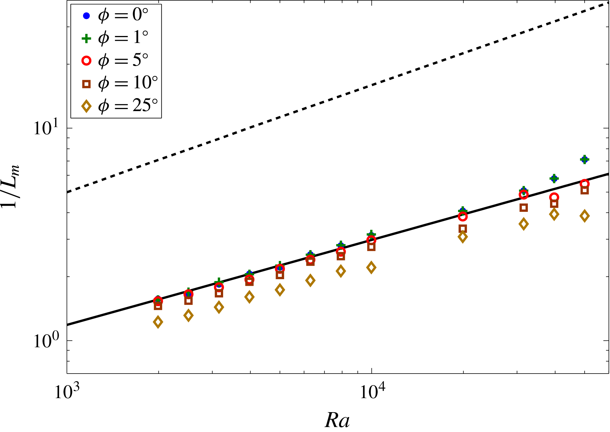
Figure 8. Variation of time-mean interplume spacing (
 $L_{m}$
) with
$L_{m}$
) with
 $Ra$
and
$Ra$
and
 $\unicode[STIX]{x1D719}$
.
$\unicode[STIX]{x1D719}$
.
 $L_{m}$
is computed by time-averaging the horizontal projection of the wall-parallel (
$L_{m}$
is computed by time-averaging the horizontal projection of the wall-parallel (
 $x$
) wavelength of the most energetic Fourier mode at the mid-plane
$x$
) wavelength of the most energetic Fourier mode at the mid-plane
 $z=0.5$
(see, for example, figures 14
b and 21
g), i.e.
$z=0.5$
(see, for example, figures 14
b and 21
g), i.e.
 $L_{m}=\langle L\cos \unicode[STIX]{x1D719}/n_{d}\rangle$
, where
$L_{m}=\langle L\cos \unicode[STIX]{x1D719}/n_{d}\rangle$
, where
 $n_{d}$
is the mode number of the dominant wall-parallel mode. The dashed line reproduces the inverse-wavelength scaling (
$n_{d}$
is the mode number of the dominant wall-parallel mode. The dashed line reproduces the inverse-wavelength scaling (
 ${\sim}Ra^{1/2}$
) of the marginal energy stability mode for
${\sim}Ra^{1/2}$
) of the marginal energy stability mode for
 $\unicode[STIX]{x1D719}=0^{\circ }$
from figure 4(b); the solid line reproduces the mean interplume spacing
$\unicode[STIX]{x1D719}=0^{\circ }$
from figure 4(b); the solid line reproduces the mean interplume spacing
 $L_{m}=(2\unicode[STIX]{x03C0}/0.47)Ra^{-0.4}$
fit to data extracted from the DNS of Hewitt et al. (Reference Hewitt, Neufeld and Lister2012) at
$L_{m}=(2\unicode[STIX]{x03C0}/0.47)Ra^{-0.4}$
fit to data extracted from the DNS of Hewitt et al. (Reference Hewitt, Neufeld and Lister2012) at
 $\unicode[STIX]{x1D719}=0^{\circ }$
; and the symbols denote data points taken from the DNS in the present study for various values of
$\unicode[STIX]{x1D719}=0^{\circ }$
; and the symbols denote data points taken from the DNS in the present study for various values of
 $\unicode[STIX]{x1D719}$
. The same aspect ratio
$\unicode[STIX]{x1D719}$
. The same aspect ratio
 $L$
as in Wen et al. (Reference Wen, Corson and Chini2015b
) (i.e. a domain sufficiently wide to encompass more than 15 pairs of plumes at
$L$
as in Wen et al. (Reference Wen, Corson and Chini2015b
) (i.e. a domain sufficiently wide to encompass more than 15 pairs of plumes at
 $\unicode[STIX]{x1D719}=0^{\circ }$
) is used here, and for each
$\unicode[STIX]{x1D719}=0^{\circ }$
) is used here, and for each
 $Ra$
the statistically steady fields from simulations performed at smaller
$Ra$
the statistically steady fields from simulations performed at smaller
 $\unicode[STIX]{x1D719}$
are utilised as the initial conditions for simulations at larger
$\unicode[STIX]{x1D719}$
are utilised as the initial conditions for simulations at larger
 $\unicode[STIX]{x1D719}$
. It can be seen that as
$\unicode[STIX]{x1D719}$
. It can be seen that as
 $\unicode[STIX]{x1D719}$
is increased the time-mean interplume spacing also is substantially increased for each
$\unicode[STIX]{x1D719}$
is increased the time-mean interplume spacing also is substantially increased for each
 $Ra$
.
$Ra$
.
An important question concerns the variation of the time-mean interplume spacing
 $L_{m}$
with
$L_{m}$
with
 $Ra$
and
$Ra$
and
 $\unicode[STIX]{x1D719}$
in the high-
$\unicode[STIX]{x1D719}$
in the high-
 $Ra$
regime. From figure 8, it can be concluded that, for fixed
$Ra$
regime. From figure 8, it can be concluded that, for fixed
 $\unicode[STIX]{x1D719}$
, the mean interplume spacing decreases as the Rayleigh number is increased at a rate bounded above by
$\unicode[STIX]{x1D719}$
, the mean interplume spacing decreases as the Rayleigh number is increased at a rate bounded above by
 $Ra^{-1/2}$
as in the horizontal case and, for finite
$Ra^{-1/2}$
as in the horizontal case and, for finite
 $\unicode[STIX]{x1D719}$
, as anticipated by the wavenumber scaling of the marginal energy stability mode (figure 4
b). Moreover, when the inclination is sufficiently small, e.g.
$\unicode[STIX]{x1D719}$
, as anticipated by the wavenumber scaling of the marginal energy stability mode (figure 4
b). Moreover, when the inclination is sufficiently small, e.g.
 $\unicode[STIX]{x1D719}=1^{\circ }$
,
$\unicode[STIX]{x1D719}=1^{\circ }$
,
 $L_{m}$
essentially remains unchanged. However, for each fixed
$L_{m}$
essentially remains unchanged. However, for each fixed
 $Ra$
, as
$Ra$
, as
 $\unicode[STIX]{x1D719}$
is increased the time-mean spacing between neighbouring interior plumes also is substantially increased. To clearly describe this pattern coarsening process, DNS initialised using a metastable, highly ordered columnar flow computed for horizontal PMC at
$\unicode[STIX]{x1D719}$
is increased the time-mean spacing between neighbouring interior plumes also is substantially increased. To clearly describe this pattern coarsening process, DNS initialised using a metastable, highly ordered columnar flow computed for horizontal PMC at
 $Ra=50\,000$
are performed for inclined PMC at the same
$Ra=50\,000$
are performed for inclined PMC at the same
 $Ra$
. As shown in figure 9, initially there exist 17 pairs of narrow columnar plumes (each consisting of a single rising and descending interior plume), which are statistically steady in the horizontal case. However, when the layer is inclined, the narrow plumes become distorted (see figure 9
b), and subsequently become unstable: as is evident in figure 9(c,d), there are localised regions in which cold plumes overlie hot ones and, as time evolves, the narrow plumes are broken down and merge to form wider ones (see figure 9
e,f). This process, namely, distorted narrow columnar flow
$Ra$
. As shown in figure 9, initially there exist 17 pairs of narrow columnar plumes (each consisting of a single rising and descending interior plume), which are statistically steady in the horizontal case. However, when the layer is inclined, the narrow plumes become distorted (see figure 9
b), and subsequently become unstable: as is evident in figure 9(c,d), there are localised regions in which cold plumes overlie hot ones and, as time evolves, the narrow plumes are broken down and merge to form wider ones (see figure 9
e,f). This process, namely, distorted narrow columnar flow
 $\rightarrow$
instability
$\rightarrow$
instability
 $\rightarrow$
wider columnar flow, is robust in inclined PMC when the mean interplume spacing is too small. The physical mechanisms underlying this trend of increasing
$\rightarrow$
wider columnar flow, is robust in inclined PMC when the mean interplume spacing is too small. The physical mechanisms underlying this trend of increasing
 $L_{m}$
with increasing
$L_{m}$
with increasing
 $\unicode[STIX]{x1D719}$
at large
$\unicode[STIX]{x1D719}$
at large
 $Ra$
will be discussed in detail in § 5.
$Ra$
will be discussed in detail in § 5.
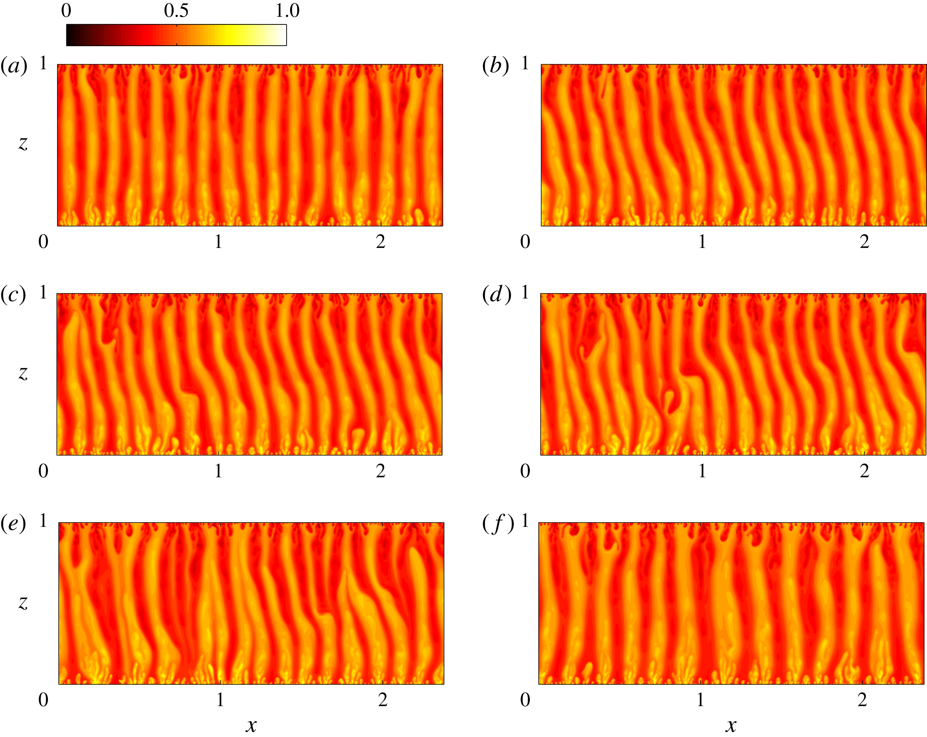
Figure 9. Snapshots of temperature fields from DNS showing the coarsening process of the columnar flow in inclined PMC at
 $Ra=50\,000$
,
$Ra=50\,000$
,
 $\unicode[STIX]{x1D719}=5^{\circ }$
and
$\unicode[STIX]{x1D719}=5^{\circ }$
and
 $L=2.387$
: (a)
$L=2.387$
: (a)
 ${\mathcal{T}}=0$
; (b)
${\mathcal{T}}=0$
; (b)
 ${\mathcal{T}}=47.4$
; (c)
${\mathcal{T}}=47.4$
; (c)
 ${\mathcal{T}}=51.15$
; (d)
${\mathcal{T}}=51.15$
; (d)
 ${\mathcal{T}}=53.4$
; (e)
${\mathcal{T}}=53.4$
; (e)
 ${\mathcal{T}}=59.25$
; and (f)
${\mathcal{T}}=59.25$
; and (f)
 ${\mathcal{T}}=495$
, where the convective time
${\mathcal{T}}=495$
, where the convective time
 ${\mathcal{T}}\equiv Ra\,t$
. Statistically steady fields extracted from DNS of horizontal PMC at the same
${\mathcal{T}}\equiv Ra\,t$
. Statistically steady fields extracted from DNS of horizontal PMC at the same
 $Ra$
and
$Ra$
and
 $L$
are utilised as initial conditions. As time evolves, 17 pairs of narrow columnar plumes are distorted, then become unstable, and finally merge into 13 pairs of wider columnar plumes.
$L$
are utilised as initial conditions. As time evolves, 17 pairs of narrow columnar plumes are distorted, then become unstable, and finally merge into 13 pairs of wider columnar plumes.
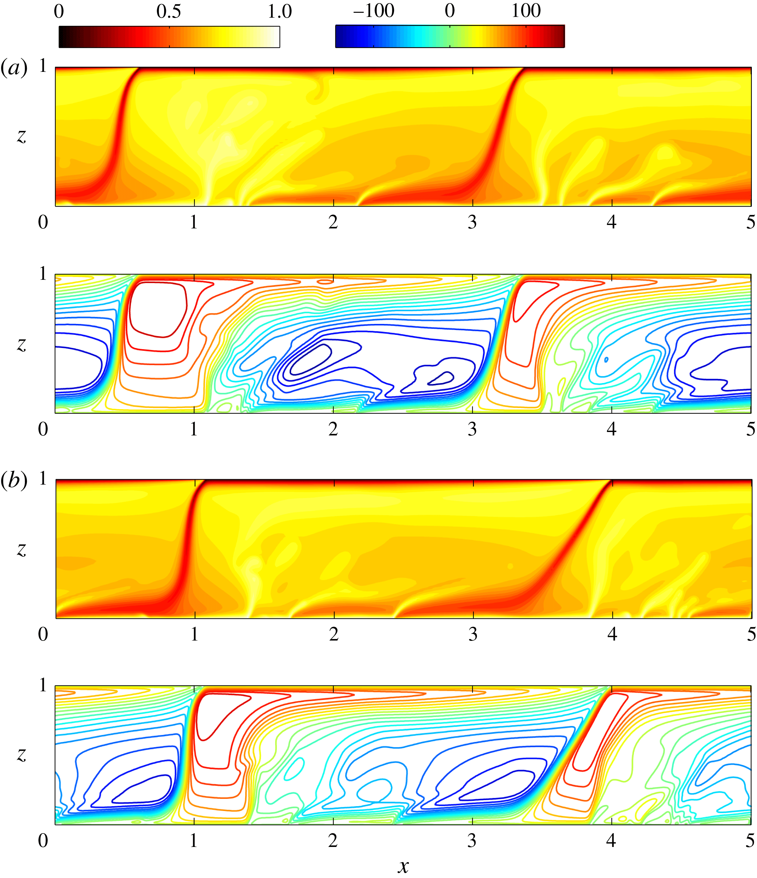
Figure 10. Large-scale convective travelling wave. Snapshots of temperature fields (upper panels) and corresponding streamlines (lower panels) for TW I from DNS at
 $Ra=9976$
,
$Ra=9976$
,
 $L=5.01$
and
$L=5.01$
and
 $\unicode[STIX]{x1D719}=32^{\circ }$
. Time evolves from (a)
$\unicode[STIX]{x1D719}=32^{\circ }$
. Time evolves from (a)
 ${\mathcal{T}}=575.17$
to (b)
${\mathcal{T}}=575.17$
to (b)
 ${\mathcal{T}}=624.06$
. For TW I, there exist four large-scale cells in the domain: two natural rolls (red
${\mathcal{T}}=624.06$
. For TW I, there exist four large-scale cells in the domain: two natural rolls (red
 $\unicode[STIX]{x1D713}$
) and two antinatural rolls (blue
$\unicode[STIX]{x1D713}$
) and two antinatural rolls (blue
 $\unicode[STIX]{x1D713}$
). The lower boundary layers of the antinatural rolls are unstable: small plumes generated from the heated wall owing to the boundary-layer instability are continually swept to the left (
$\unicode[STIX]{x1D713}$
). The lower boundary layers of the antinatural rolls are unstable: small plumes generated from the heated wall owing to the boundary-layer instability are continually swept to the left (
 $-x$
) and merge with the large-scale hot plumes. The natural rolls are tightly attached to the cooled wall, the upper boundary layer is stable, and as time evolves the entire flow pattern moves to the right (
$-x$
) and merge with the large-scale hot plumes. The natural rolls are tightly attached to the cooled wall, the upper boundary layer is stable, and as time evolves the entire flow pattern moves to the right (
 $+x$
).
$+x$
).
As shown in figure 10, there is a fundamental change in the structure of the convection at large
 $Ra$
when
$Ra$
when
 $\unicode[STIX]{x1D719}\approx 32^{\circ }$
, with the flow transitioning to a large-scale travelling-wave (TW) state. Unlike the quasicoherent cellular flows arising at moderate
$\unicode[STIX]{x1D719}\approx 32^{\circ }$
, with the flow transitioning to a large-scale travelling-wave (TW) state. Unlike the quasicoherent cellular flows arising at moderate
 $Ra$
in horizontal PMC, however, the resulting large-scale convective flow at
$Ra$
in horizontal PMC, however, the resulting large-scale convective flow at
 $Ra=9976$
and
$Ra=9976$
and
 $\unicode[STIX]{x1D719}=32^{\circ }$
manifests as one of two types of quasirelative periodic orbits (i.e. quasitime-periodic flow structures travelling at some velocity in
$\unicode[STIX]{x1D719}=32^{\circ }$
manifests as one of two types of quasirelative periodic orbits (i.e. quasitime-periodic flow structures travelling at some velocity in
 $\pm x$
) that lack statistical centrosymmetry, hereafter referred to as TW I and TW II (see figures 10 and 11). For each flow state, there exist four large-scale (two natural and two antinatural) rolls in a domain with
$\pm x$
) that lack statistical centrosymmetry, hereafter referred to as TW I and TW II (see figures 10 and 11). For each flow state, there exist four large-scale (two natural and two antinatural) rolls in a domain with
 $L=5.01$
, and the natural rolls are tightly attached either to the upper wall (see figure 10) or to the lower wall (see figure 11), with a stable upper or lower boundary layer, respectively. Near the opposite walls (the lower for TW I and upper for TW II), small-scale protoplumes quasiperiodically grow from the unstable boundary layers, and are continually swept into and merge with the large-scale plumes in the interior. Interestingly, for both TW I and II, the large-scale wave pattern travels in the direction opposite to that of the protoplumes.
$L=5.01$
, and the natural rolls are tightly attached either to the upper wall (see figure 10) or to the lower wall (see figure 11), with a stable upper or lower boundary layer, respectively. Near the opposite walls (the lower for TW I and upper for TW II), small-scale protoplumes quasiperiodically grow from the unstable boundary layers, and are continually swept into and merge with the large-scale plumes in the interior. Interestingly, for both TW I and II, the large-scale wave pattern travels in the direction opposite to that of the protoplumes.
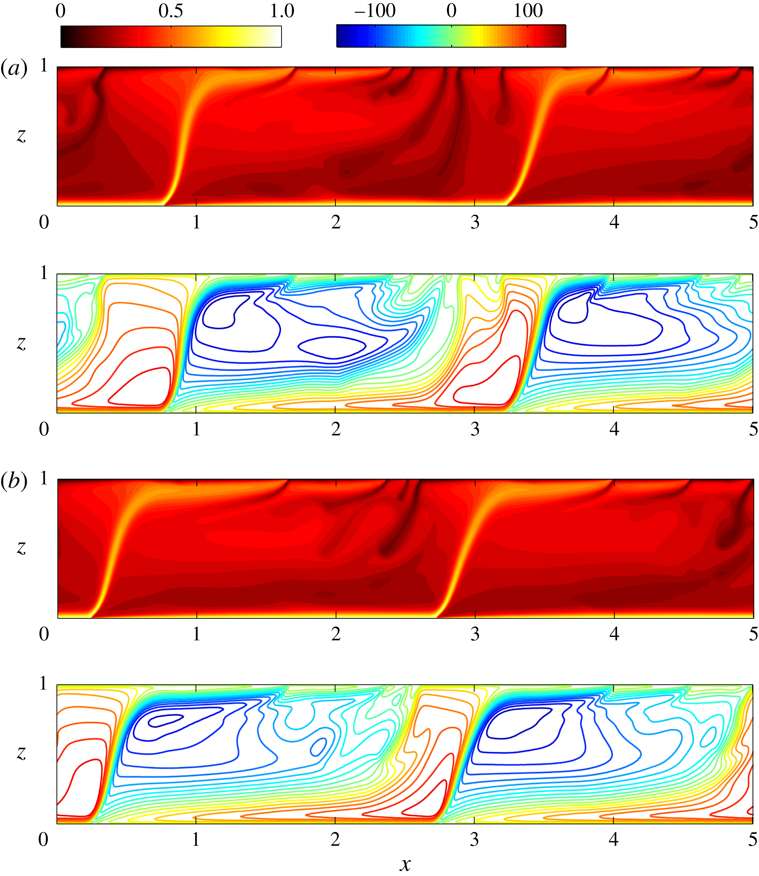
Figure 11. Large-scale convective travelling wave. Snapshots of temperature fields (upper panels) and corresponding streamlines (lower panels) for TW II from DNS at
 $Ra=9976$
,
$Ra=9976$
,
 $L=5.01$
and
$L=5.01$
and
 $\unicode[STIX]{x1D719}=32^{\circ }$
. Time evolves from (a)
$\unicode[STIX]{x1D719}=32^{\circ }$
. Time evolves from (a)
 ${\mathcal{T}}=502.81$
to (b)
${\mathcal{T}}=502.81$
to (b)
 ${\mathcal{T}}=551.69$
. For TW II, there also exist four large-scale cells in the domain: two natural rolls (red
${\mathcal{T}}=551.69$
. For TW II, there also exist four large-scale cells in the domain: two natural rolls (red
 $\unicode[STIX]{x1D713}$
) and two antinatural rolls (blue
$\unicode[STIX]{x1D713}$
) and two antinatural rolls (blue
 $\unicode[STIX]{x1D713}$
). However, unlike TW I, the upper boundary layers of the antinatural rolls are unstable: small plumes generated from the cooled wall owing to the boundary-layer instability are continually swept to the right (
$\unicode[STIX]{x1D713}$
). However, unlike TW I, the upper boundary layers of the antinatural rolls are unstable: small plumes generated from the cooled wall owing to the boundary-layer instability are continually swept to the right (
 $+x$
) and merge with the large-scale cold plumes. The natural rolls are tightly attached to the heated wall, the lower boundary layer is stable, and as time evolves the entire flow pattern moves to the left (
$+x$
) and merge with the large-scale cold plumes. The natural rolls are tightly attached to the heated wall, the lower boundary layer is stable, and as time evolves the entire flow pattern moves to the left (
 $-x$
).
$-x$
).
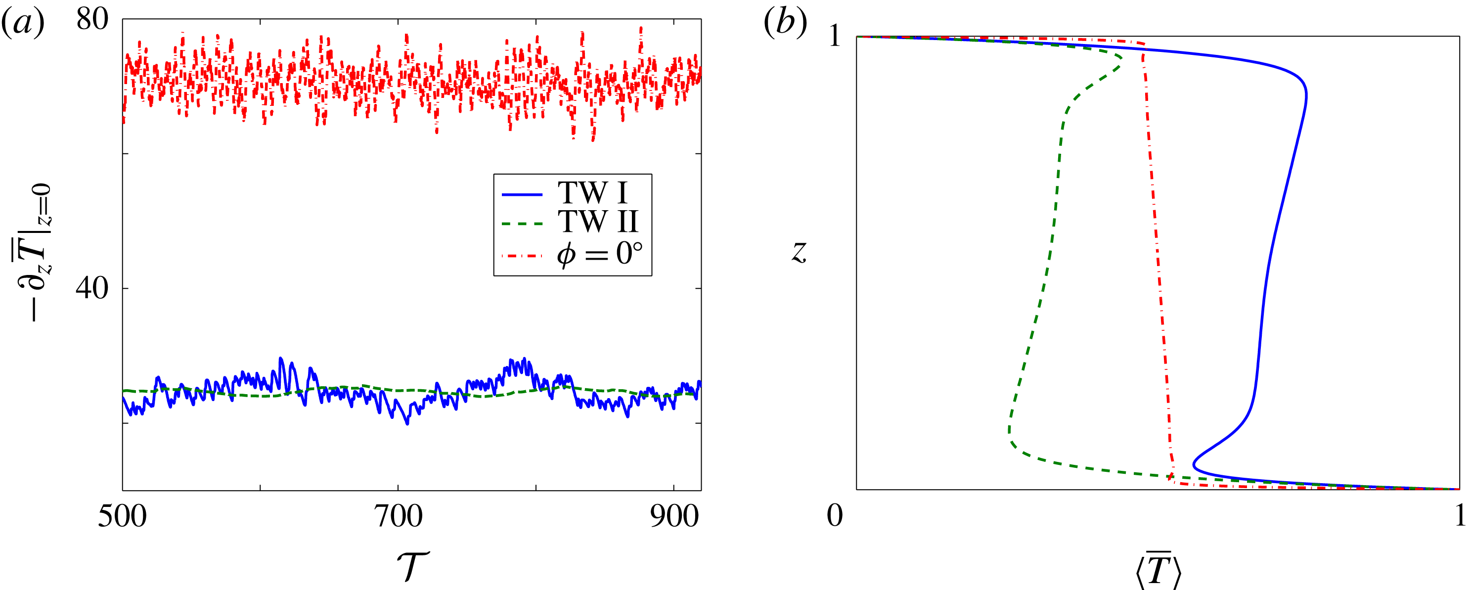
Figure 12. Time series of the instantaneous Nusselt number
 $-\unicode[STIX]{x2202}_{z}\overline{T}|_{z=0}$
and the time- and wall-parallel-mean temperature profiles
$-\unicode[STIX]{x2202}_{z}\overline{T}|_{z=0}$
and the time- and wall-parallel-mean temperature profiles
 $\langle \overline{T}\rangle$
from DNS at
$\langle \overline{T}\rangle$
from DNS at
 $Ra=9976$
,
$Ra=9976$
,
 $L=5.01$
and
$L=5.01$
and
 $\unicode[STIX]{x1D719}=32^{\circ }$
. (a) Variation of
$\unicode[STIX]{x1D719}=32^{\circ }$
. (a) Variation of
 $-\unicode[STIX]{x2202}_{z}\overline{T}|_{z=0}$
with convective time
$-\unicode[STIX]{x2202}_{z}\overline{T}|_{z=0}$
with convective time
 ${\mathcal{T}}=Ra\,t$
for both TW I and TW II. (b) Neither mean temperature profile (TW I or TW II) is antisymmetric about the mid-plane. Nevertheless,
${\mathcal{T}}=Ra\,t$
for both TW I and TW II. (b) Neither mean temperature profile (TW I or TW II) is antisymmetric about the mid-plane. Nevertheless,
 $Nu=24.7$
for both TW I and II. For reference, the corresponding results for
$Nu=24.7$
for both TW I and II. For reference, the corresponding results for
 $\unicode[STIX]{x1D719}=0^{\circ }$
are also plotted.
$\unicode[STIX]{x1D719}=0^{\circ }$
are also plotted.
Figure 12 shows the time series of the instantaneous Nusselt number
 $-\unicode[STIX]{x2202}_{z}\overline{T}|_{z=0}$
and the time- and wall-parallel-mean temperature profiles
$-\unicode[STIX]{x2202}_{z}\overline{T}|_{z=0}$
and the time- and wall-parallel-mean temperature profiles
 $\langle \overline{T}\rangle$
for these two states at
$\langle \overline{T}\rangle$
for these two states at
 $\unicode[STIX]{x1D719}=32^{\circ }$
. Clearly, the instantaneous Nusselt number varies less vigorously for both TW I and TW II than it does for the columnar flow realised at
$\unicode[STIX]{x1D719}=32^{\circ }$
. Clearly, the instantaneous Nusselt number varies less vigorously for both TW I and TW II than it does for the columnar flow realised at
 $\unicode[STIX]{x1D719}=0^{\circ }$
. Moreover, the mean temperature profile for each state exhibits a loss of antisymmetry about the mid-plane (
$\unicode[STIX]{x1D719}=0^{\circ }$
. Moreover, the mean temperature profile for each state exhibits a loss of antisymmetry about the mid-plane (
 $z=0.5$
). For TW I, the hot plume occupies a majority of the area of the interior domain so that the magnitude of
$z=0.5$
). For TW I, the hot plume occupies a majority of the area of the interior domain so that the magnitude of
 $\langle \overline{T}\rangle$
is greater than
$\langle \overline{T}\rangle$
is greater than
 $1/2$
in the core; conversely, for TW II, the cold plume dominates the interior so that the magnitude of
$1/2$
in the core; conversely, for TW II, the cold plume dominates the interior so that the magnitude of
 $\langle \overline{T}\rangle$
is less than
$\langle \overline{T}\rangle$
is less than
 $1/2$
in the core. These two states transport heat at the same rate, however, as evident in figure 12.
$1/2$
in the core. These two states transport heat at the same rate, however, as evident in figure 12.
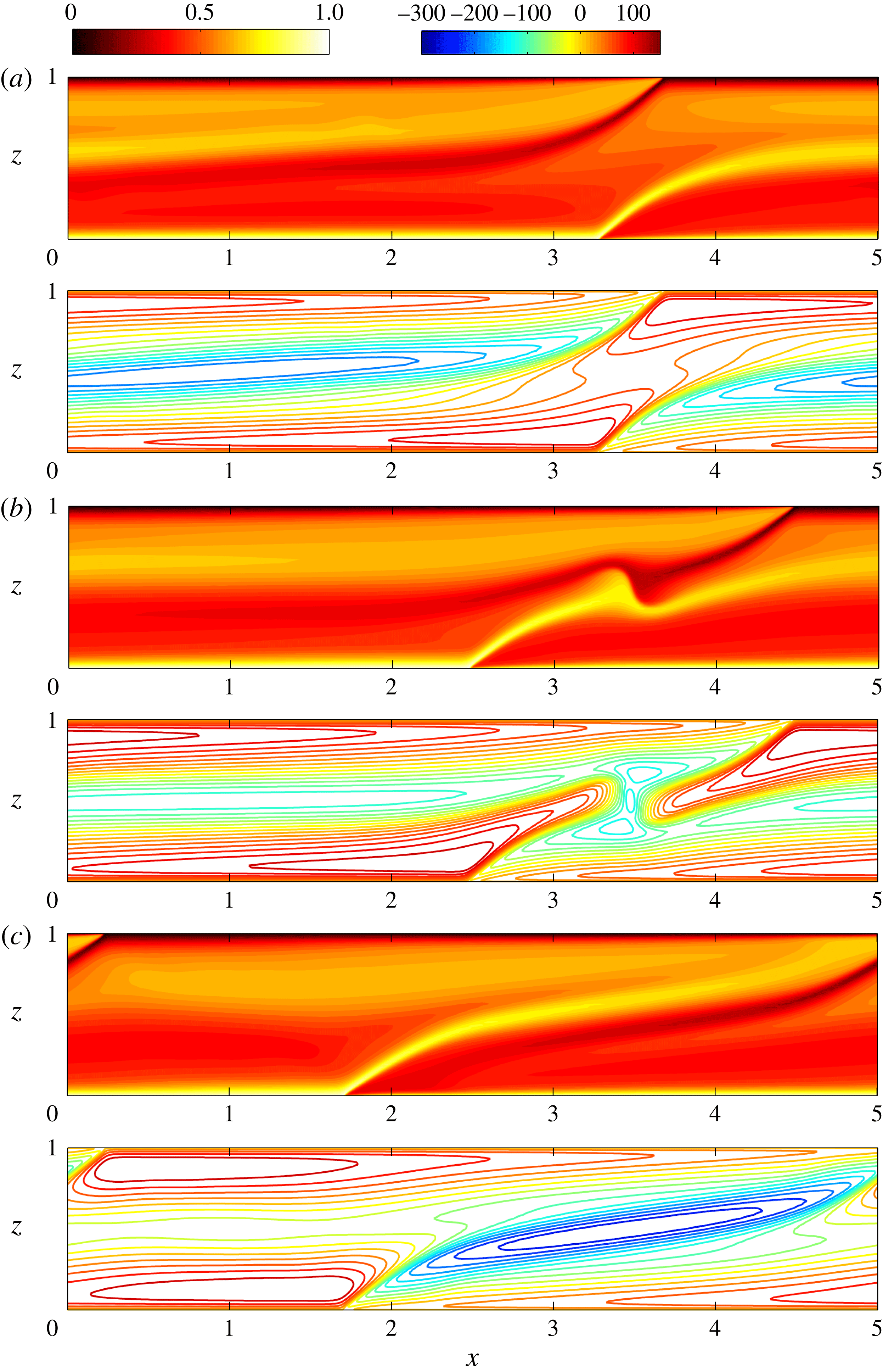
Figure 13. Modified large-scale convective travelling wave. Snapshots of temperature fields (upper panels) and corresponding streamlines (lower panels) from DNS at
 $Ra=9976$
,
$Ra=9976$
,
 $L=5.01$
and
$L=5.01$
and
 $\unicode[STIX]{x1D719}=35^{\circ }$
. Time evolves from panel (a)
$\unicode[STIX]{x1D719}=35^{\circ }$
. Time evolves from panel (a)
 ${\mathcal{T}}=1393.89$
to (b)
${\mathcal{T}}=1393.89$
to (b)
 ${\mathcal{T}}=1424.62$
to (c)
${\mathcal{T}}=1424.62$
to (c)
 ${\mathcal{T}}=1439.98$
. The hot (rising) plume is travelling to the left while the cold (descending) plume propagates to the right. At some instant, the plumes collide and then exchange their positions.
${\mathcal{T}}=1439.98$
. The hot (rising) plume is travelling to the left while the cold (descending) plume propagates to the right. At some instant, the plumes collide and then exchange their positions.
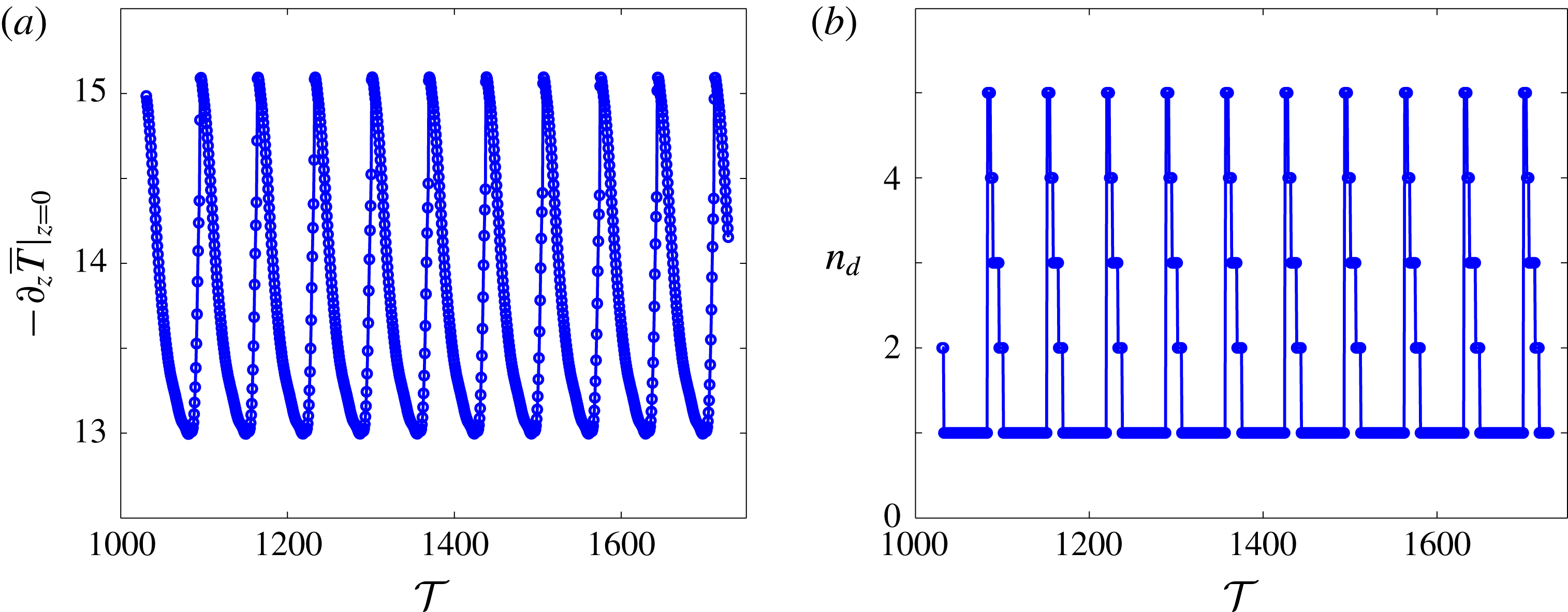
Figure 14. Time series of instantaneous (a) Nusselt number
 $-\unicode[STIX]{x2202}_{z}\overline{T}|_{z=0}$
and (b) dominant wall-parallel mode number
$-\unicode[STIX]{x2202}_{z}\overline{T}|_{z=0}$
and (b) dominant wall-parallel mode number
 $n_{d}$
in the core (
$n_{d}$
in the core (
 $z=0.5$
) at
$z=0.5$
) at
 $Ra=9976$
,
$Ra=9976$
,
 $L=5.01$
and
$L=5.01$
and
 $\unicode[STIX]{x1D719}=35^{\circ }$
. In these plots,
$\unicode[STIX]{x1D719}=35^{\circ }$
. In these plots,
 $-\unicode[STIX]{x2202}_{z}\overline{T}|_{z=0}$
and
$-\unicode[STIX]{x2202}_{z}\overline{T}|_{z=0}$
and
 $n_{d}$
vary periodically with the convective time
$n_{d}$
vary periodically with the convective time
 ${\mathcal{T}}$
defined as in figure 12. In the domain interior, the flow consists of several Fourier modes but is dominated by the first mode (
${\mathcal{T}}$
defined as in figure 12. In the domain interior, the flow consists of several Fourier modes but is dominated by the first mode (
 $n_{d}=1$
) except when the two plumes collide.
$n_{d}=1$
) except when the two plumes collide.
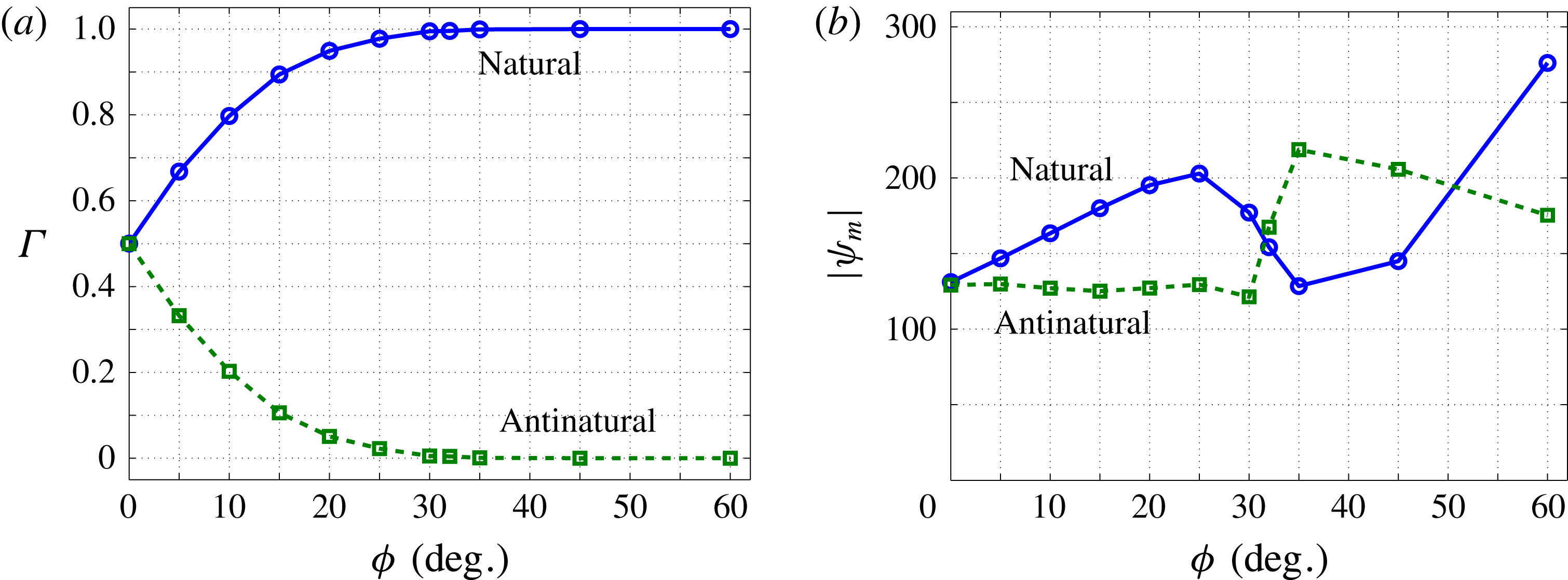
Figure 15. Statistical properties of the natural and antinatural rolls at
 $Ra=9976$
as a function of inclination angle. (a)
$Ra=9976$
as a function of inclination angle. (a)
 $\unicode[STIX]{x1D6E4}$
denotes the fractional contact area of the natural/antinatural roll at the first Chebyshev grid points near the upper and lower walls:
$\unicode[STIX]{x1D6E4}$
denotes the fractional contact area of the natural/antinatural roll at the first Chebyshev grid points near the upper and lower walls:
 $\unicode[STIX]{x1D6E4}=L_{{\unicode[STIX]{x1D713}>0\atop \unicode[STIX]{x1D713}<0}}/L$
is formed using the
$\unicode[STIX]{x1D6E4}=L_{{\unicode[STIX]{x1D713}>0\atop \unicode[STIX]{x1D713}<0}}/L$
is formed using the
 $\unicode[STIX]{x1D713}$
data (
$\unicode[STIX]{x1D713}$
data (
 $\unicode[STIX]{x1D713}>0$
for the natural roll and
$\unicode[STIX]{x1D713}>0$
for the natural roll and
 $\unicode[STIX]{x1D713}<0$
for the antinatural roll) at these grid points. As the inclination of the layer is increased, the antinatural rolls gradually become detached from the walls, while the natural rolls attach to the walls ever more tightly. (b)
$\unicode[STIX]{x1D713}<0$
for the antinatural roll) at these grid points. As the inclination of the layer is increased, the antinatural rolls gradually become detached from the walls, while the natural rolls attach to the walls ever more tightly. (b)
 $|\unicode[STIX]{x1D713}_{m}|$
denotes the magnitude of extremum
$|\unicode[STIX]{x1D713}_{m}|$
denotes the magnitude of extremum
 $\unicode[STIX]{x1D713}$
value for the natural/antinatural roll. For
$\unicode[STIX]{x1D713}$
value for the natural/antinatural roll. For
 $\unicode[STIX]{x1D719}\leqslant 25^{\circ }$
, the extremum
$\unicode[STIX]{x1D719}\leqslant 25^{\circ }$
, the extremum
 $\unicode[STIX]{x1D713}$
value for the natural rolls increases almost linearly, while this value for the antinatural rolls remains nearly constant. However, the flow structure changes dramatically for
$\unicode[STIX]{x1D713}$
value for the natural rolls increases almost linearly, while this value for the antinatural rolls remains nearly constant. However, the flow structure changes dramatically for
 $25^{\circ }<\unicode[STIX]{x1D719}<35^{\circ }$
.
$25^{\circ }<\unicode[STIX]{x1D719}<35^{\circ }$
.
The four-cell convective flows depicted in figures 10 and 11 propagate strictly in one direction (
 $+x$
or
$+x$
or
 $-x$
). For
$-x$
). For
 $\unicode[STIX]{x1D719}\gtrsim 35^{\circ }$
, there is a transition to a large-scale two-cell convective state in which the natural and antinatural rolls travel in opposite directions. As shown in figure 13, the hot and cold plumes are strained in the wall-parallel direction under the effect of inclined buoyancy. During the straining process, the root of the cold/hot plume is pushed by the hot/cold plume towards the
$\unicode[STIX]{x1D719}\gtrsim 35^{\circ }$
, there is a transition to a large-scale two-cell convective state in which the natural and antinatural rolls travel in opposite directions. As shown in figure 13, the hot and cold plumes are strained in the wall-parallel direction under the effect of inclined buoyancy. During the straining process, the root of the cold/hot plume is pushed by the hot/cold plume towards the
 $+x/-x$
direction (see figure 13
a). At a particular instant, the two plumes meet, then collide and thus interchange their relative positions (see figure 13
b). In a sufficiently wide,
$+x/-x$
direction (see figure 13
a). At a particular instant, the two plumes meet, then collide and thus interchange their relative positions (see figure 13
b). In a sufficiently wide,
 $L$
-periodic domain, this process occurs time-periodically for
$L$
-periodic domain, this process occurs time-periodically for
 $5000\leqslant Ra\leqslant 9976$
(see figure 14) and becomes spatiotemporally chaotic for
$5000\leqslant Ra\leqslant 9976$
(see figure 14) and becomes spatiotemporally chaotic for
 $Ra>9976$
. The time scale of these large-scale travelling-wave flows for
$Ra>9976$
. The time scale of these large-scale travelling-wave flows for
 $\unicode[STIX]{x1D719}\gtrsim 32^{\circ }$
is much larger than the convective eddy turnover time of the three-region columnar flows arising for
$\unicode[STIX]{x1D719}\gtrsim 32^{\circ }$
is much larger than the convective eddy turnover time of the three-region columnar flows arising for
 $\unicode[STIX]{x1D719}\lesssim 25^{\circ }$
; i.e. the unsteadiness induced by the travelling-wave flow is relatively mild.
$\unicode[STIX]{x1D719}\lesssim 25^{\circ }$
; i.e. the unsteadiness induced by the travelling-wave flow is relatively mild.
To quantitatively describe how the flow structure changes with the inclination angle of the layer at large Rayleigh number, we measured the fractional contact area
 $\unicode[STIX]{x1D6E4}$
of the natural and antinatural rolls near the upper and lower walls and the magnitude of the extremum
$\unicode[STIX]{x1D6E4}$
of the natural and antinatural rolls near the upper and lower walls and the magnitude of the extremum
 $\unicode[STIX]{x1D713}$
values for these rolls at different inclination angles. As shown in figure 15(a), as
$\unicode[STIX]{x1D713}$
values for these rolls at different inclination angles. As shown in figure 15(a), as
 $\unicode[STIX]{x1D719}$
is increased, the contact area between the antinatural rolls and two walls decreases monotonically; i.e. the antinatural rolls gradually detach from the walls. Specifically,
$\unicode[STIX]{x1D719}$
is increased, the contact area between the antinatural rolls and two walls decreases monotonically; i.e. the antinatural rolls gradually detach from the walls. Specifically,
 $\unicode[STIX]{x1D6E4}$
decreases to
$\unicode[STIX]{x1D6E4}$
decreases to
 $2.2\,\%$
at
$2.2\,\%$
at
 $\unicode[STIX]{x1D719}=25^{\circ }$
and to
$\unicode[STIX]{x1D719}=25^{\circ }$
and to
 $0.1\,\%$
at
$0.1\,\%$
at
 $\unicode[STIX]{x1D719}=35^{\circ }$
, with the antinatural rolls then making contact with the heated and cooled walls only at certain localised points. Concomitantly, the natural rolls become attached to the walls more tightly. Figure 15(b) indicates that for
$\unicode[STIX]{x1D719}=35^{\circ }$
, with the antinatural rolls then making contact with the heated and cooled walls only at certain localised points. Concomitantly, the natural rolls become attached to the walls more tightly. Figure 15(b) indicates that for
 $\unicode[STIX]{x1D719}\leqslant 25^{\circ }$
the inclination of the layer intensifies the natural-roll motions. Although the inclination of the layer should also suppress the antinatural-roll motions, the DNS reveal that the magnitude of the extremum
$\unicode[STIX]{x1D719}\leqslant 25^{\circ }$
the inclination of the layer intensifies the natural-roll motions. Although the inclination of the layer should also suppress the antinatural-roll motions, the DNS reveal that the magnitude of the extremum
 $\unicode[STIX]{x1D713}$
value for the antinatural roll remains nearly constant for
$\unicode[STIX]{x1D713}$
value for the antinatural roll remains nearly constant for
 $\unicode[STIX]{x1D719}\leqslant 25^{\circ }$
. This is partly because, as
$\unicode[STIX]{x1D719}\leqslant 25^{\circ }$
. This is partly because, as
 $\unicode[STIX]{x1D719}$
is increased, the interior plumes widen (e.g. see figure 8) and the rolls strengthen, which increases the extremum
$\unicode[STIX]{x1D719}$
is increased, the interior plumes widen (e.g. see figure 8) and the rolls strengthen, which increases the extremum
 $\unicode[STIX]{x1D713}$
value to a certain extent.
$\unicode[STIX]{x1D713}$
value to a certain extent.
In summary, our DNS show that for
 $0^{\circ }<\unicode[STIX]{x1D719}\lesssim 25^{\circ }$
the flow at large
$0^{\circ }<\unicode[STIX]{x1D719}\lesssim 25^{\circ }$
the flow at large
 $Ra$
exhibits a three-region columnar structure similar to that arising in the horizontal case. When the inclination angle
$Ra$
exhibits a three-region columnar structure similar to that arising in the horizontal case. When the inclination angle
 $\unicode[STIX]{x1D719}$
exceeds some critical value
$\unicode[STIX]{x1D719}$
exceeds some critical value
 $\unicode[STIX]{x1D719}_{t}$
, the columnar flow structure is completely broken down and the flow then transitions to a large-scale travelling-wave convective roll state (see figures 10, 11 and 13). We have performed DNS at other large values of
$\unicode[STIX]{x1D719}_{t}$
, the columnar flow structure is completely broken down and the flow then transitions to a large-scale travelling-wave convective roll state (see figures 10, 11 and 13). We have performed DNS at other large values of
 $Ra$
that also confirm this trend and suggest that
$Ra$
that also confirm this trend and suggest that
 $30^{\circ }<\unicode[STIX]{x1D719}_{t}<32^{\circ }$
independently of
$30^{\circ }<\unicode[STIX]{x1D719}_{t}<32^{\circ }$
independently of
 $Ra$
once
$Ra$
once
 $Ra$
is sufficiently large: namely, for
$Ra$
is sufficiently large: namely, for
 $\unicode[STIX]{x1D719}\leqslant 30^{\circ }$
, the convection takes the form of a three-region turbulent flow, while for
$\unicode[STIX]{x1D719}\leqslant 30^{\circ }$
, the convection takes the form of a three-region turbulent flow, while for
 $\unicode[STIX]{x1D719}\geqslant 32^{\circ }$
, the convection transitions to a large-scale travelling-wave convective flow. Interestingly, as discussed in § 3.1, the linear stability analysis performed by Rees & Bassom (Reference Rees and Bassom2000) also predicts a transition angle
$\unicode[STIX]{x1D719}\geqslant 32^{\circ }$
, the convection transitions to a large-scale travelling-wave convective flow. Interestingly, as discussed in § 3.1, the linear stability analysis performed by Rees & Bassom (Reference Rees and Bassom2000) also predicts a transition angle
 $\unicode[STIX]{x1D719}_{t}=31.30^{\circ }$
above which the basic state is linearly stable to 2D disturbances for all
$\unicode[STIX]{x1D719}_{t}=31.30^{\circ }$
above which the basic state is linearly stable to 2D disturbances for all
 $Ra$
. Although it is not yet clear whether these two transition angles are precisely equivalent, our data suggest that they are at least very close.
$Ra$
. Although it is not yet clear whether these two transition angles are precisely equivalent, our data suggest that they are at least very close.
Table 1. Prefactors
 $C$
in the
$C$
in the
 $Nu\sim CRa$
scaling relationship obtained from DNS (for
$Nu\sim CRa$
scaling relationship obtained from DNS (for
 $0^{\circ }\leqslant \unicode[STIX]{x1D719}\leqslant 30^{\circ }$
) and variational upper-bound analysis (for
$0^{\circ }\leqslant \unicode[STIX]{x1D719}\leqslant 30^{\circ }$
) and variational upper-bound analysis (for
 $0^{\circ }\leqslant \unicode[STIX]{x1D719}\leqslant 90^{\circ }$
) in the high-
$0^{\circ }\leqslant \unicode[STIX]{x1D719}\leqslant 90^{\circ }$
) in the high-
 $Ra$
regime. In the DNS, the prefactor is increased approximately by
$Ra$
regime. In the DNS, the prefactor is increased approximately by
 $2.2\,\%$
at
$2.2\,\%$
at
 $\unicode[STIX]{x1D719}=10^{\circ }$
; however, in the variational upper-bound analysis, the prefactors for both the predictions and the upper bounds monotonically decrease as
$\unicode[STIX]{x1D719}=10^{\circ }$
; however, in the variational upper-bound analysis, the prefactors for both the predictions and the upper bounds monotonically decrease as
 $\unicode[STIX]{x1D719}$
is increased.
$\unicode[STIX]{x1D719}$
is increased.
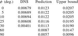
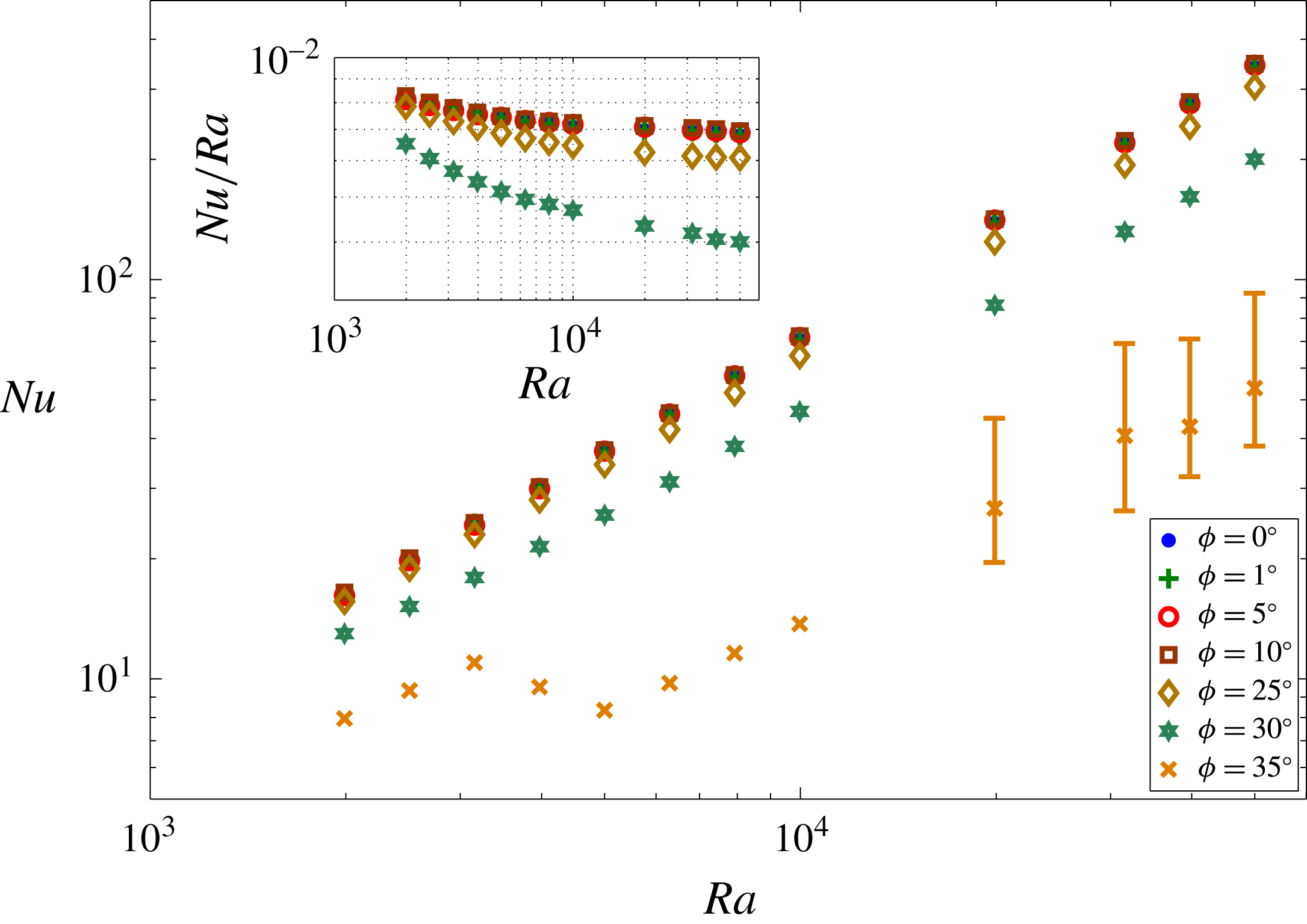
Figure 16. Variation of
 $Nu$
with
$Nu$
with
 $Ra$
and
$Ra$
and
 $\unicode[STIX]{x1D719}$
in the high-
$\unicode[STIX]{x1D719}$
in the high-
 $Ra$
regime. The inset shows the scaled
$Ra$
regime. The inset shows the scaled
 $Nu$
for
$Nu$
for
 $\unicode[STIX]{x1D719}\leqslant 30^{\circ }$
. At large
$\unicode[STIX]{x1D719}\leqslant 30^{\circ }$
. At large
 $Ra$
, the heat transport is nearly unaffected by the inclination of the layer until
$Ra$
, the heat transport is nearly unaffected by the inclination of the layer until
 $\unicode[STIX]{x1D719}\geqslant 25^{\circ }$
. For
$\unicode[STIX]{x1D719}\geqslant 25^{\circ }$
. For
 $\unicode[STIX]{x1D719}\leqslant 30^{\circ }$
,
$\unicode[STIX]{x1D719}\leqslant 30^{\circ }$
,
 $Nu\sim CRa$
as
$Nu\sim CRa$
as
 $Ra\rightarrow \infty$
with the prefactors shown in table 1. The sharp change in
$Ra\rightarrow \infty$
with the prefactors shown in table 1. The sharp change in
 $Nu$
at
$Nu$
at
 $\unicode[STIX]{x1D719}=35^{\circ }$
for
$\unicode[STIX]{x1D719}=35^{\circ }$
for
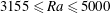 $3155\leqslant Ra\leqslant 5000$
is due to the flow transition from a four-cell pattern at
$3155\leqslant Ra\leqslant 5000$
is due to the flow transition from a four-cell pattern at
 $Ra=3155$
, as in figures 10 and 11, to a similar two-cell pattern at
$Ra=3155$
, as in figures 10 and 11, to a similar two-cell pattern at
 $Ra=3972$
, and then to another two-cell pattern as in figure 13 for
$Ra=3972$
, and then to another two-cell pattern as in figure 13 for
 $Ra\geqslant 5000$
. For
$Ra\geqslant 5000$
. For
 $Ra\geqslant 19\,905$
and at
$Ra\geqslant 19\,905$
and at
 $\unicode[STIX]{x1D719}=35^{\circ }$
, the slow large-scale convective motions require extremely long computing times to obtain accurate values of
$\unicode[STIX]{x1D719}=35^{\circ }$
, the slow large-scale convective motions require extremely long computing times to obtain accurate values of
 $Nu$
, so error bars are included to show the range of variation of the instantaneous Nusselt number in these computations (for which the averaging times are not sufficiently long).
$Nu$
, so error bars are included to show the range of variation of the instantaneous Nusselt number in these computations (for which the averaging times are not sufficiently long).
4.2 Heat transport
Figure 16 shows the variation of
 $Nu$
with
$Nu$
with
 $Ra$
and
$Ra$
and
 $\unicode[STIX]{x1D719}$
at large Rayleigh number. For
$\unicode[STIX]{x1D719}$
at large Rayleigh number. For
 $\unicode[STIX]{x1D719}\leqslant 10^{\circ }$
(actually
$\unicode[STIX]{x1D719}\leqslant 10^{\circ }$
(actually
 $\unicode[STIX]{x1D719}\lesssim 20^{\circ }$
as shown in figure 17
a),
$\unicode[STIX]{x1D719}\lesssim 20^{\circ }$
as shown in figure 17
a),
 $Nu$
is nearly independent of
$Nu$
is nearly independent of
 $\unicode[STIX]{x1D719}$
. For
$\unicode[STIX]{x1D719}$
. For
 $\unicode[STIX]{x1D719}\geqslant 25^{\circ }$
, however, the antinatural rolls begin to detach from the upper and lower walls, so that the organised columnar flow structure is destroyed and less heat is transported. Moreover, when
$\unicode[STIX]{x1D719}\geqslant 25^{\circ }$
, however, the antinatural rolls begin to detach from the upper and lower walls, so that the organised columnar flow structure is destroyed and less heat is transported. Moreover, when
 $\unicode[STIX]{x1D719}>\unicode[STIX]{x1D719}_{t}$
, where
$\unicode[STIX]{x1D719}>\unicode[STIX]{x1D719}_{t}$
, where
 $30^{\circ }<\unicode[STIX]{x1D719}_{t}<32^{\circ }$
, the columnar flow structure is completely broken down: the flow transitions to the large-scale travelling-wave convective roll state, and the heat transport is significantly reduced. More precisely, the DNS indicate that for
$30^{\circ }<\unicode[STIX]{x1D719}_{t}<32^{\circ }$
, the columnar flow structure is completely broken down: the flow transitions to the large-scale travelling-wave convective roll state, and the heat transport is significantly reduced. More precisely, the DNS indicate that for
 $\unicode[STIX]{x1D719}\leqslant 30^{\circ }$
,
$\unicode[STIX]{x1D719}\leqslant 30^{\circ }$
,
 $Nu\sim CRa$
with a
$Nu\sim CRa$
with a
 $\unicode[STIX]{x1D719}$
-dependent prefactor
$\unicode[STIX]{x1D719}$
-dependent prefactor
 $C$
(see table 1). Owing to the extremely long computing times (more than
$C$
(see table 1). Owing to the extremely long computing times (more than
 $10^{4}$
convective time units) required to ensure a converged value of
$10^{4}$
convective time units) required to ensure a converged value of
 $Nu$
is obtained, it is unclear whether this linear scaling with
$Nu$
is obtained, it is unclear whether this linear scaling with
 $Ra$
holds for
$Ra$
holds for
 $\unicode[STIX]{x1D719}\geqslant 35^{\circ }$
.
$\unicode[STIX]{x1D719}\geqslant 35^{\circ }$
.
Figure 17. Variation of (a)
 $Nu$
and (b)
$Nu$
and (b)
 $\langle \overline{T}\rangle$
with
$\langle \overline{T}\rangle$
with
 $\unicode[STIX]{x1D719}$
at
$\unicode[STIX]{x1D719}$
at
 $Ra=9976$
and
$Ra=9976$
and
 $L=5.01$
. (a)
$L=5.01$
. (a)
 $Nu$
is only weakly dependent on
$Nu$
is only weakly dependent on
 $\unicode[STIX]{x1D719}$
for
$\unicode[STIX]{x1D719}$
for
 $\unicode[STIX]{x1D719}\lesssim 20^{\circ }$
, although there is a slight increase up to a maximum around
$\unicode[STIX]{x1D719}\lesssim 20^{\circ }$
, although there is a slight increase up to a maximum around
 $\unicode[STIX]{x1D719}=10^{\circ }$
. For
$\unicode[STIX]{x1D719}=10^{\circ }$
. For
 $\unicode[STIX]{x1D719}\geqslant 25^{\circ }$
, the columnar flow structure begins to break down and
$\unicode[STIX]{x1D719}\geqslant 25^{\circ }$
, the columnar flow structure begins to break down and
 $Nu$
decreases rapidly as
$Nu$
decreases rapidly as
 $\unicode[STIX]{x1D719}$
is increased further. (b) The primary features of the mean temperature profile at
$\unicode[STIX]{x1D719}$
is increased further. (b) The primary features of the mean temperature profile at
 $\unicode[STIX]{x1D719}=0^{\circ }$
are retained for
$\unicode[STIX]{x1D719}=0^{\circ }$
are retained for
 $\unicode[STIX]{x1D719}\leqslant 30^{\circ }$
.
$\unicode[STIX]{x1D719}\leqslant 30^{\circ }$
.
Figure 17 shows the variation of both
 $Nu$
and
$Nu$
and
 $\langle \overline{T}\rangle$
with
$\langle \overline{T}\rangle$
with
 $\unicode[STIX]{x1D719}$
at
$\unicode[STIX]{x1D719}$
at
 $Ra=9976$
. Interestingly, the variation of
$Ra=9976$
. Interestingly, the variation of
 $Nu$
with
$Nu$
with
 $\unicode[STIX]{x1D719}$
at large Rayleigh number (figure 17
a) exhibits a very similar trend to that computed by Caltagirone & Bories (Reference Caltagirone and Bories1985) at
$\unicode[STIX]{x1D719}$
at large Rayleigh number (figure 17
a) exhibits a very similar trend to that computed by Caltagirone & Bories (Reference Caltagirone and Bories1985) at
 $Ra=100$
except that the flow patterns reported here are quite different. For instance, as
$Ra=100$
except that the flow patterns reported here are quite different. For instance, as
 $\unicode[STIX]{x1D719}$
is increased, the flow at large
$\unicode[STIX]{x1D719}$
is increased, the flow at large
 $Ra$
transitions from a turbulent columnar flow to a large-scale travelling-wave state, while in Caltagirone & Bories (Reference Caltagirone and Bories1985) the flow at
$Ra$
transitions from a turbulent columnar flow to a large-scale travelling-wave state, while in Caltagirone & Bories (Reference Caltagirone and Bories1985) the flow at
 $Ra=100$
changes from a multicellular steady state to the basic unicellular state. Moreover, it is seen in figure 17(a) that moderate inclination of the layer slightly enhances the heat transport (also see table 1). Finally, figure 17(b) indicates that for
$Ra=100$
changes from a multicellular steady state to the basic unicellular state. Moreover, it is seen in figure 17(a) that moderate inclination of the layer slightly enhances the heat transport (also see table 1). Finally, figure 17(b) indicates that for
 $\unicode[STIX]{x1D719}\leqslant 30^{\circ }$
the main characteristics of the mean temperature profiles, including the emergence of thin thermal boundary layers and an unstably stratified core, are unchanged relative to the horizontal case. At
$\unicode[STIX]{x1D719}\leqslant 30^{\circ }$
the main characteristics of the mean temperature profiles, including the emergence of thin thermal boundary layers and an unstably stratified core, are unchanged relative to the horizontal case. At
 $\unicode[STIX]{x1D719}=35^{\circ }$
, however, the core becomes stably stratified.
$\unicode[STIX]{x1D719}=35^{\circ }$
, however, the core becomes stably stratified.
5 Mechanisms: structure and stability of steady convective solutions
The DNS described in § 4 reveal that the instantaneous flow self-organises into different recurrent quasicoherent structures at large
 $Ra$
, i.e. narrow columnar plumes and large-scale travelling waves, suggesting that the basic physics can be understood by studying related exact coherent states: steady, periodic orbit and/or travelling-wave solutions of the governing equations. In horizontal porous medium convection, the studies of steady columnar flows by Hewitt, Neufeld & Lister (Reference Hewitt, Neufeld and Lister2013), Wen et al. (Reference Wen, Corson and Chini2015b
) and Hewitt & Lister (Reference Hewitt and Lister2017) do, indeed, shed light on the development of high-
$Ra$
, i.e. narrow columnar plumes and large-scale travelling waves, suggesting that the basic physics can be understood by studying related exact coherent states: steady, periodic orbit and/or travelling-wave solutions of the governing equations. In horizontal porous medium convection, the studies of steady columnar flows by Hewitt, Neufeld & Lister (Reference Hewitt, Neufeld and Lister2013), Wen et al. (Reference Wen, Corson and Chini2015b
) and Hewitt & Lister (Reference Hewitt and Lister2017) do, indeed, shed light on the development of high-
 $Ra$
spatiotemporally chaotic convection. In this section, the structure and stability of steady nonlinear convective states are investigated numerically to gain a more detailed mechanistic insight into the physics of inclined PMC at large
$Ra$
spatiotemporally chaotic convection. In this section, the structure and stability of steady nonlinear convective states are investigated numerically to gain a more detailed mechanistic insight into the physics of inclined PMC at large
 $Ra$
and relatively modest
$Ra$
and relatively modest
 $\unicode[STIX]{x1D719}$
.
$\unicode[STIX]{x1D719}$
.
5.1 Steady convective states
The steady version of the governing equations (2.10)–(2.11) can be solved numerically using a Newton-GMRES (generalised minimal residual) iterative scheme. First, following the Newton–Kantorovich formulation used by Wen et al. (Reference Wen, Corson and Chini2015b ) to compute steady convective states in horizontal PMC, we express the linear differential equations for the corrections in the inclined case as
 $$\begin{eqnarray}\displaystyle \left[\begin{array}{@{}cc@{}}\unicode[STIX]{x1D6FB}^{2} & Ra(\cos \unicode[STIX]{x1D719}D_{x}-\sin \unicode[STIX]{x1D719}D_{z})\\ -D_{x}+\unicode[STIX]{x1D703}_{z}^{i}D_{x}-\unicode[STIX]{x1D703}_{x}^{i}D_{z} & \unicode[STIX]{x1D6FB}^{2}-\unicode[STIX]{x1D713}_{z}^{i}D_{x}+\unicode[STIX]{x1D713}_{x}^{i}D_{z}\end{array}\right]\left[\begin{array}{@{}c@{}}\unicode[STIX]{x0394}^{\unicode[STIX]{x1D713}}\\ \unicode[STIX]{x0394}^{\unicode[STIX]{x1D703}}\end{array}\right]=\left[\begin{array}{@{}c@{}}-F_{res}^{\unicode[STIX]{x1D713}}\\ -F_{res}^{\unicode[STIX]{x1D703}}\end{array}\right]^{i}, & & \displaystyle\end{eqnarray}$$
where the superscript
 $i$
denotes the
$i$
denotes the
 $i$
th Newton iterate;
$i$
th Newton iterate;
 $D_{x}$
and
$D_{x}$
and
 $D_{z}$
denote the first partial derivative operators with respect to
$D_{z}$
denote the first partial derivative operators with respect to
 $x$
and
$x$
and
 $z$
; the correction terms
$z$
; the correction terms
 $\unicode[STIX]{x0394}^{\unicode[STIX]{x1D713}}$
and
$\unicode[STIX]{x0394}^{\unicode[STIX]{x1D713}}$
and
 $\unicode[STIX]{x0394}^{\unicode[STIX]{x1D703}}$
are defined by
$\unicode[STIX]{x0394}^{\unicode[STIX]{x1D703}}$
are defined by
 $$\begin{eqnarray}\displaystyle \unicode[STIX]{x0394}^{\unicode[STIX]{x1D713}}=\unicode[STIX]{x1D713}^{i+1}-\unicode[STIX]{x1D713}^{i},\quad \unicode[STIX]{x0394}^{\unicode[STIX]{x1D703}}=\unicode[STIX]{x1D703}^{i+1}-\unicode[STIX]{x1D703}^{i}; & & \displaystyle\end{eqnarray}$$
and
 $$\begin{eqnarray}\displaystyle & \displaystyle F_{res}^{\unicode[STIX]{x1D713}}=\unicode[STIX]{x1D6FB}^{2}\unicode[STIX]{x1D713}+Ra(\cos \unicode[STIX]{x1D719}\unicode[STIX]{x2202}_{x}-\sin \unicode[STIX]{x1D719}\unicode[STIX]{x2202}_{z})\unicode[STIX]{x1D703}+Ra\sin \unicode[STIX]{x1D719}, & \displaystyle\end{eqnarray}$$
 $$\begin{eqnarray}\displaystyle & \displaystyle F_{res}^{\unicode[STIX]{x1D703}}=\unicode[STIX]{x1D6FB}^{2}\unicode[STIX]{x1D703}-(\unicode[STIX]{x2202}_{z}\unicode[STIX]{x1D713}\unicode[STIX]{x2202}_{x}\unicode[STIX]{x1D703}-\unicode[STIX]{x2202}_{x}\unicode[STIX]{x1D713}\unicode[STIX]{x2202}_{z}\unicode[STIX]{x1D703}+\unicode[STIX]{x2202}_{x}\unicode[STIX]{x1D713}) & \displaystyle\end{eqnarray}$$
correspond to the residuals of the steady governing equations. To simplify the iterative scheme,
 $F_{res}^{\unicode[STIX]{x1D713}}$
can be set to
$F_{res}^{\unicode[STIX]{x1D713}}$
can be set to
 $0$
since, for a given
$0$
since, for a given
 $\unicode[STIX]{x0394}^{\unicode[STIX]{x1D703}}$
,
$\unicode[STIX]{x0394}^{\unicode[STIX]{x1D703}}$
,
 $\unicode[STIX]{x0394}^{\unicode[STIX]{x1D713}}$
can be obtained by solving
$\unicode[STIX]{x0394}^{\unicode[STIX]{x1D713}}$
can be obtained by solving
 $$\begin{eqnarray}\displaystyle \unicode[STIX]{x1D6FB}^{2}\unicode[STIX]{x0394}^{\unicode[STIX]{x1D713}}=Ra(\sin \unicode[STIX]{x1D719}D_{z}-\cos \unicode[STIX]{x1D719}D_{x})\unicode[STIX]{x0394}^{\unicode[STIX]{x1D703}}. & & \displaystyle\end{eqnarray}$$
Thus, (5.1) becomes
 $$\begin{eqnarray}\displaystyle \left[\begin{array}{@{}cc@{}}-D_{x}+\unicode[STIX]{x1D703}_{z}^{i}D_{x}-\unicode[STIX]{x1D703}_{x}^{i}D_{z} & \unicode[STIX]{x1D6FB}^{2}-\unicode[STIX]{x1D713}_{z}^{i}D_{x}+\unicode[STIX]{x1D713}_{x}^{i}D_{z}\end{array}\right]\left[\begin{array}{@{}c@{}}\unicode[STIX]{x0394}^{\unicode[STIX]{x1D713}}\\ \unicode[STIX]{x0394}^{\unicode[STIX]{x1D703}}\end{array}\right]=\left[\begin{array}{@{}c@{}}-F_{res}^{\unicode[STIX]{x1D703}}\end{array}\right]^{i}, & & \displaystyle\end{eqnarray}$$
and the only unknown is
 $\unicode[STIX]{x0394}^{\unicode[STIX]{x1D703}}$
. For a given wall-parallel wavenumber
$\unicode[STIX]{x0394}^{\unicode[STIX]{x1D703}}$
. For a given wall-parallel wavenumber
 $nk_{s}$
(where
$nk_{s}$
(where
 $k_{s}$
is the fundamental wavenumber of the spatially periodic steady solution), (5.6) becomes
$k_{s}$
is the fundamental wavenumber of the spatially periodic steady solution), (5.6) becomes
 $$\begin{eqnarray}\displaystyle \hat{\mathbb{L}}_{n}^{i}(\unicode[STIX]{x0394}^{\unicode[STIX]{x1D703}})=\hat{f}_{n}^{i}, & & \displaystyle\end{eqnarray}$$
where
 $\hat{\mathbb{L}}_{n}^{i}$
and
$\hat{\mathbb{L}}_{n}^{i}$
and
 $\hat{f}_{n}^{i}$
represent the Fourier coefficients of the left- and right-hand sides of (5.6) at the
$\hat{f}_{n}^{i}$
represent the Fourier coefficients of the left- and right-hand sides of (5.6) at the
 $i$
th Newton iterate, respectively. For each Newton iterate, (5.7) is solved iteratively in the Krylov subspace using the GMRES method (Trefethen & Bau Reference Trefethen and Bau1997). Spatial discretisation in
$i$
th Newton iterate, respectively. For each Newton iterate, (5.7) is solved iteratively in the Krylov subspace using the GMRES method (Trefethen & Bau Reference Trefethen and Bau1997). Spatial discretisation in
 $z$
is achieved using a Chebyshev spectral collocation method. In order to improve the convergence rate of the GMRES iterations, a preconditioner
$z$
is achieved using a Chebyshev spectral collocation method. In order to improve the convergence rate of the GMRES iterations, a preconditioner
 $\unicode[STIX]{x1D648}=\unicode[STIX]{x1D6FB}^{2}$
is chosen for solving (5.7). Hence the actual computational linear algebra problem is
$\unicode[STIX]{x1D648}=\unicode[STIX]{x1D6FB}^{2}$
is chosen for solving (5.7). Hence the actual computational linear algebra problem is
 $$\begin{eqnarray}\displaystyle \hat{\unicode[STIX]{x1D648}}_{n}^{-1}\hat{\mathbb{L}}_{n}^{i}(\unicode[STIX]{x0394}^{\unicode[STIX]{x1D703}})=\hat{\unicode[STIX]{x1D648}}_{n}^{-1}\hat{f}_{n}^{i}, & & \displaystyle\end{eqnarray}$$
where
 $\hat{\unicode[STIX]{x1D648}}_{n}$
is the matrix of Fourier coefficients of
$\hat{\unicode[STIX]{x1D648}}_{n}$
is the matrix of Fourier coefficients of
 $\unicode[STIX]{x1D648}$
for the mode with wall-parallel wavenumber
$\unicode[STIX]{x1D648}$
for the mode with wall-parallel wavenumber
 $nk_{s}$
: namely,
$nk_{s}$
: namely,
 $\hat{\unicode[STIX]{x1D648}}_{n}=D_{zz}-(nk_{s})^{2}\unicode[STIX]{x1D644}$
. Although reflection symmetry is not realised for the inclined case, the centrosymmetry still exists and requires
$\hat{\unicode[STIX]{x1D648}}_{n}=D_{zz}-(nk_{s})^{2}\unicode[STIX]{x1D644}$
. Although reflection symmetry is not realised for the inclined case, the centrosymmetry still exists and requires
 $$\begin{eqnarray}\displaystyle a_{mn}\;\text{is imaginary if}\;(m+n)\;\text{is even};\;\text{otherwise, for odd}\;(m+n),\;a_{mn}\;\text{is real}. & & \displaystyle\end{eqnarray}$$
The above centrosymmetry constraint is enforced in the computations. Moreover, the GMRES iteration is stopped once the
 $L^{2}$
-norm of the residual of (5.8) is less than
$L^{2}$
-norm of the residual of (5.8) is less than
 $10^{-4}$
, and then
$10^{-4}$
, and then
 $\hat{\unicode[STIX]{x1D703}}_{n}$
is updated. Finally, the Newton iteration is stopped when the
$\hat{\unicode[STIX]{x1D703}}_{n}$
is updated. Finally, the Newton iteration is stopped when the
 $L^{2}$
-norm of
$L^{2}$
-norm of
 $F_{res}^{\unicode[STIX]{x1D703}}$
is less than
$F_{res}^{\unicode[STIX]{x1D703}}$
is less than
 $10^{-8}$
.
$10^{-8}$
.
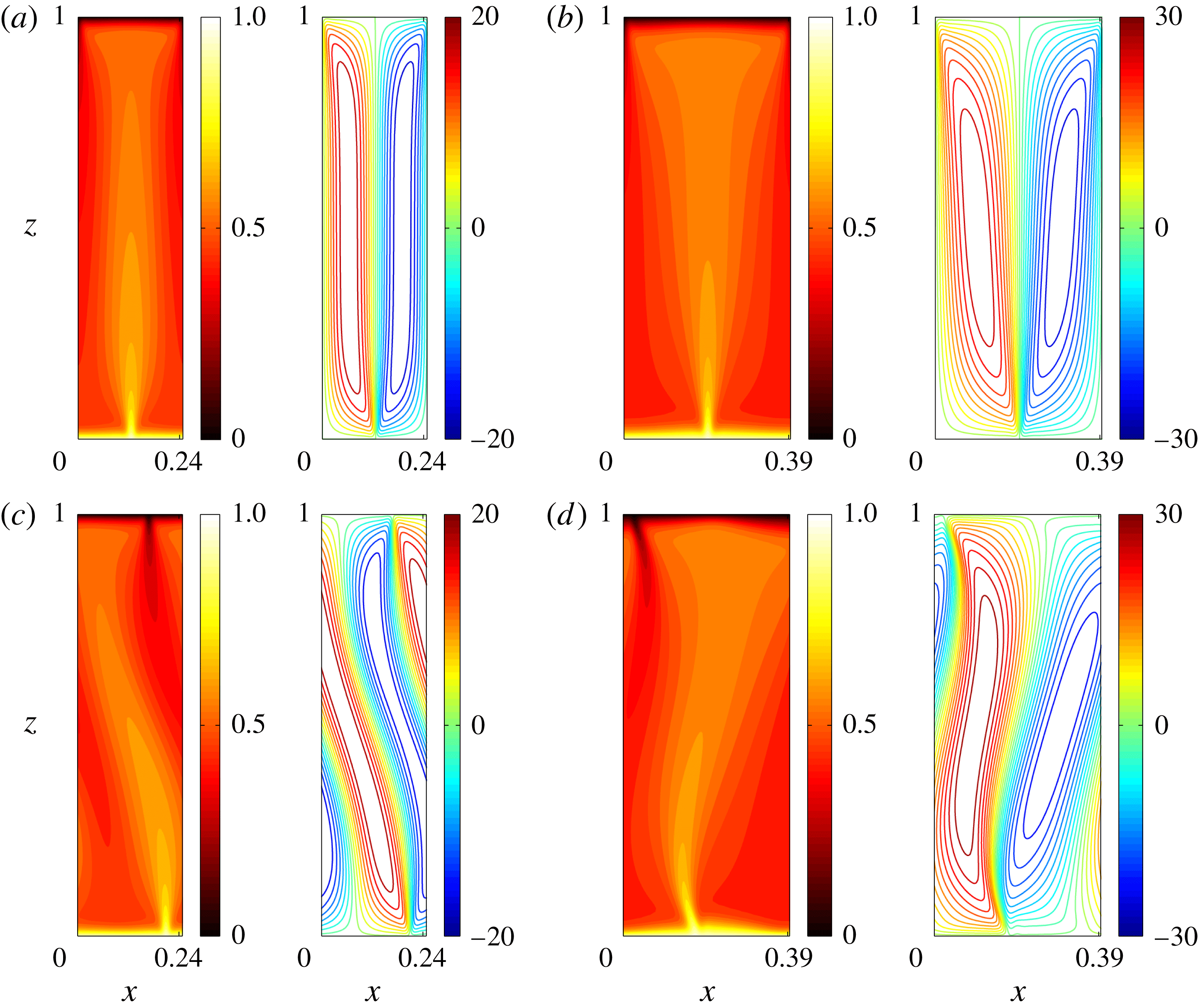
Figure 18. Steady-state temperature fields (left panels) and corresponding streamlines (right panels) at
 $Ra=5000$
: (a)
$Ra=5000$
: (a)
 $\unicode[STIX]{x1D719}=0^{\circ }$
,
$\unicode[STIX]{x1D719}=0^{\circ }$
,
 $L_{s}=0.251$
; (b)
$L_{s}=0.251$
; (b)
 $\unicode[STIX]{x1D719}=0^{\circ }$
,
$\unicode[STIX]{x1D719}=0^{\circ }$
,
 $L_{s}=0.398$
; (c)
$L_{s}=0.398$
; (c)
 $\unicode[STIX]{x1D719}=0.96^{\circ }$
,
$\unicode[STIX]{x1D719}=0.96^{\circ }$
,
 $L_{s}=0.251$
; (d)
$L_{s}=0.251$
; (d)
 $\unicode[STIX]{x1D719}=6^{\circ }$
,
$\unicode[STIX]{x1D719}=6^{\circ }$
,
 $L_{s}=0.398$
.
$L_{s}=0.398$
.
 $L_{s}=0.398$
is close to the mean interplume spacing
$L_{s}=0.398$
is close to the mean interplume spacing
 $L_{m}$
measured from the DNS at
$L_{m}$
measured from the DNS at
 $\unicode[STIX]{x1D719}=0^{\circ }$
. The magnitudes of the extremum
$\unicode[STIX]{x1D719}=0^{\circ }$
. The magnitudes of the extremum
 $\unicode[STIX]{x1D713}$
values are, for the natural rolls, (a) 19.7, (b) 27.0, (c) 20.0, (d) 29.9 and, for the antinatural rolls, (a) 19.7, (b) 27.0, (c) 18.4, (d) 25.5. Clearly, the steady convective states exhibit qualitatively different distortions for the different aspect ratios shown.
$\unicode[STIX]{x1D713}$
values are, for the natural rolls, (a) 19.7, (b) 27.0, (c) 20.0, (d) 29.9 and, for the antinatural rolls, (a) 19.7, (b) 27.0, (c) 18.4, (d) 25.5. Clearly, the steady convective states exhibit qualitatively different distortions for the different aspect ratios shown.
As shown in figure 18, the distortion of steady convective states under inclination at large
 $Ra$
depends on the aspect ratio
$Ra$
depends on the aspect ratio
 $L_{s}=2\unicode[STIX]{x03C0}/k_{s}$
. For small
$L_{s}=2\unicode[STIX]{x03C0}/k_{s}$
. For small
 $L_{s}$
, the motion of the narrow rolls is too weak to resist the impact of the background base flow. Consequently, both the natural and antinatural rolls are distorted in a counterclockwise fashion, i.e. in the same sense as the flow of the base state. However, as
$L_{s}$
, the motion of the narrow rolls is too weak to resist the impact of the background base flow. Consequently, both the natural and antinatural rolls are distorted in a counterclockwise fashion, i.e. in the same sense as the flow of the base state. However, as
 $L_{s}$
is increased, the roll motions become stronger (with larger extremum
$L_{s}$
is increased, the roll motions become stronger (with larger extremum
 $\unicode[STIX]{x1D713}$
values, see figure 18) and exhibit a qualitatively different distorted pattern for
$\unicode[STIX]{x1D713}$
values, see figure 18) and exhibit a qualitatively different distorted pattern for
 $\unicode[STIX]{x1D719}\neq 0^{\circ }$
: the natural roll is more tightly attached to the walls while the antinatural roll begins to separate from the walls. It should be noted that these two types of pattern can be readily observed in DNS for very narrowly and more widely spaced plumes.
$\unicode[STIX]{x1D719}\neq 0^{\circ }$
: the natural roll is more tightly attached to the walls while the antinatural roll begins to separate from the walls. It should be noted that these two types of pattern can be readily observed in DNS for very narrowly and more widely spaced plumes.
5.2 Secondary stability analysis
Following Wen et al. (Reference Wen, Corson and Chini2015b
), we next perform a spatial Floquet analysis to investigate the linear stability of the fully nonlinear steady convective states in an inclined porous layer. Each field is decomposed into a steady nonlinear base flow component (denoted with a subscript ‘
 $s$
’) plus a time-varying perturbation (denoted with a tilde),
$s$
’) plus a time-varying perturbation (denoted with a tilde),
 $$\begin{eqnarray}\displaystyle & \displaystyle \unicode[STIX]{x1D713}(x,z,t)=\unicode[STIX]{x1D713}_{s}(x,z)+\widetilde{\unicode[STIX]{x1D713}}(x,z,t), & \displaystyle\end{eqnarray}$$
 $$\begin{eqnarray}\displaystyle & \displaystyle T(x,z,t)=T_{s}(x,z)+\widetilde{\unicode[STIX]{x1D703}}(x,z,t), & \displaystyle\end{eqnarray}$$
where
 $T_{s}=(1-z)+\unicode[STIX]{x1D703}_{s}$
. The evolution of the small-amplitude disturbances
$T_{s}=(1-z)+\unicode[STIX]{x1D703}_{s}$
. The evolution of the small-amplitude disturbances
 $\widetilde{\unicode[STIX]{x1D713}}$
and
$\widetilde{\unicode[STIX]{x1D713}}$
and
 $\widetilde{\unicode[STIX]{x1D703}}$
is governed by the linearised system
$\widetilde{\unicode[STIX]{x1D703}}$
is governed by the linearised system
 $$\begin{eqnarray}\displaystyle & \displaystyle \unicode[STIX]{x1D6FB}^{2}\widetilde{\unicode[STIX]{x1D713}}=Ra(\sin \unicode[STIX]{x1D719}\unicode[STIX]{x2202}_{z}-\cos \unicode[STIX]{x1D719}\unicode[STIX]{x2202}_{x})\widetilde{\unicode[STIX]{x1D703}}, & \displaystyle\end{eqnarray}$$
 $$\begin{eqnarray}\displaystyle & \displaystyle \unicode[STIX]{x2202}_{t}\widetilde{\unicode[STIX]{x1D703}}=\unicode[STIX]{x1D6FB}^{2}\widetilde{\unicode[STIX]{x1D703}}-\unicode[STIX]{x2202}_{x}\unicode[STIX]{x1D703}_{s}\unicode[STIX]{x2202}_{z}\widetilde{\unicode[STIX]{x1D713}}+\unicode[STIX]{x2202}_{z}\unicode[STIX]{x1D703}_{s}\unicode[STIX]{x2202}_{x}\widetilde{\unicode[STIX]{x1D713}}+\unicode[STIX]{x2202}_{x}\unicode[STIX]{x1D713}_{s}\unicode[STIX]{x2202}_{z}\widetilde{\unicode[STIX]{x1D703}}-\unicode[STIX]{x2202}_{z}\unicode[STIX]{x1D713}_{s}\unicode[STIX]{x2202}_{x}\widetilde{\unicode[STIX]{x1D703}}-\unicode[STIX]{x2202}_{x}\widetilde{\unicode[STIX]{x1D713}}. & \displaystyle\end{eqnarray}$$
According to Floquet theory, the perturbations in (5.12) and (5.13) can be expressed as
 $$\begin{eqnarray}\displaystyle \left[\begin{array}{@{}c@{}}\widetilde{\unicode[STIX]{x1D703}}\\ \widetilde{\unicode[STIX]{x1D713}}\end{array}\right]=\text{e}^{\text{i}\unicode[STIX]{x1D6FD}k_{s}x}\left\{\mathop{\sum }_{n=-\infty }^{\infty }\left[\begin{array}{@{}c@{}}\hat{\widetilde{\unicode[STIX]{x1D703}}}_{n}(z)\\ \hat{\widetilde{\unicode[STIX]{x1D713}}}_{n}(z)\end{array}\right]\text{e}^{\text{i}nk_{s}x}\right\}\text{e}^{\unicode[STIX]{x1D706}^{\star }t}+\text{c.c.}, & & \displaystyle\end{eqnarray}$$
where
 $\unicode[STIX]{x1D706}^{\star }$
is the temporal growth rate and
$\unicode[STIX]{x1D706}^{\star }$
is the temporal growth rate and
 $\unicode[STIX]{x1D6FD}$
is the real Floquet parameter (
$\unicode[STIX]{x1D6FD}$
is the real Floquet parameter (
 $0\leqslant \unicode[STIX]{x1D6FD}\leqslant 0.5$
) that provides the freedom to modify the fundamental wall-parallel wavenumber of the perturbation. Substituting (5.14) into (5.12)–(5.13) yields
$0\leqslant \unicode[STIX]{x1D6FD}\leqslant 0.5$
) that provides the freedom to modify the fundamental wall-parallel wavenumber of the perturbation. Substituting (5.14) into (5.12)–(5.13) yields
 $$\begin{eqnarray}\displaystyle & \displaystyle -Ra[\sin \unicode[STIX]{x1D719}D_{z}-\text{i}(n+\unicode[STIX]{x1D6FD})k_{s}\cos \unicode[STIX]{x1D719}]\hat{\widetilde{\unicode[STIX]{x1D703}}}_{n}+\left[D_{zz}-(n+\unicode[STIX]{x1D6FD})^{2}k_{s}^{2}\right]\hat{\widetilde{\unicode[STIX]{x1D713}}}_{n}=0, & \displaystyle\end{eqnarray}$$
 $$\begin{eqnarray}\displaystyle & \displaystyle [D_{zz}-(n+\unicode[STIX]{x1D6FD})^{2}k_{s}^{2}+\widetilde{h}_{n}]\hat{\widetilde{\unicode[STIX]{x1D703}}}_{n}+\left[-i(n+\unicode[STIX]{x1D6FD})k_{s}+\widetilde{g}_{n}\right]\hat{\widetilde{\unicode[STIX]{x1D713}}}_{n}=\unicode[STIX]{x1D706}^{\star }\hat{\widetilde{\unicode[STIX]{x1D703}}}_{n} & \displaystyle\end{eqnarray}$$
for each wall-parallel Fourier mode (indexed by integer
 $n$
), where
$n$
), where
 $\widetilde{h}_{n}$
and
$\widetilde{h}_{n}$
and
 $\widetilde{g}_{n}$
can be determined by calculating the convolution of the non-constant-coefficient terms in (5.13). Finally, the eigenvalue problem (5.15)–(5.16) is discretised using a Chebyshev collocation method and the resulting algebraic eigenvalue problem is solved using Arnoldi iteration to obtain the leading eigenvalues and eigenfunctions.
$\widetilde{g}_{n}$
can be determined by calculating the convolution of the non-constant-coefficient terms in (5.13). Finally, the eigenvalue problem (5.15)–(5.16) is discretised using a Chebyshev collocation method and the resulting algebraic eigenvalue problem is solved using Arnoldi iteration to obtain the leading eigenvalues and eigenfunctions.
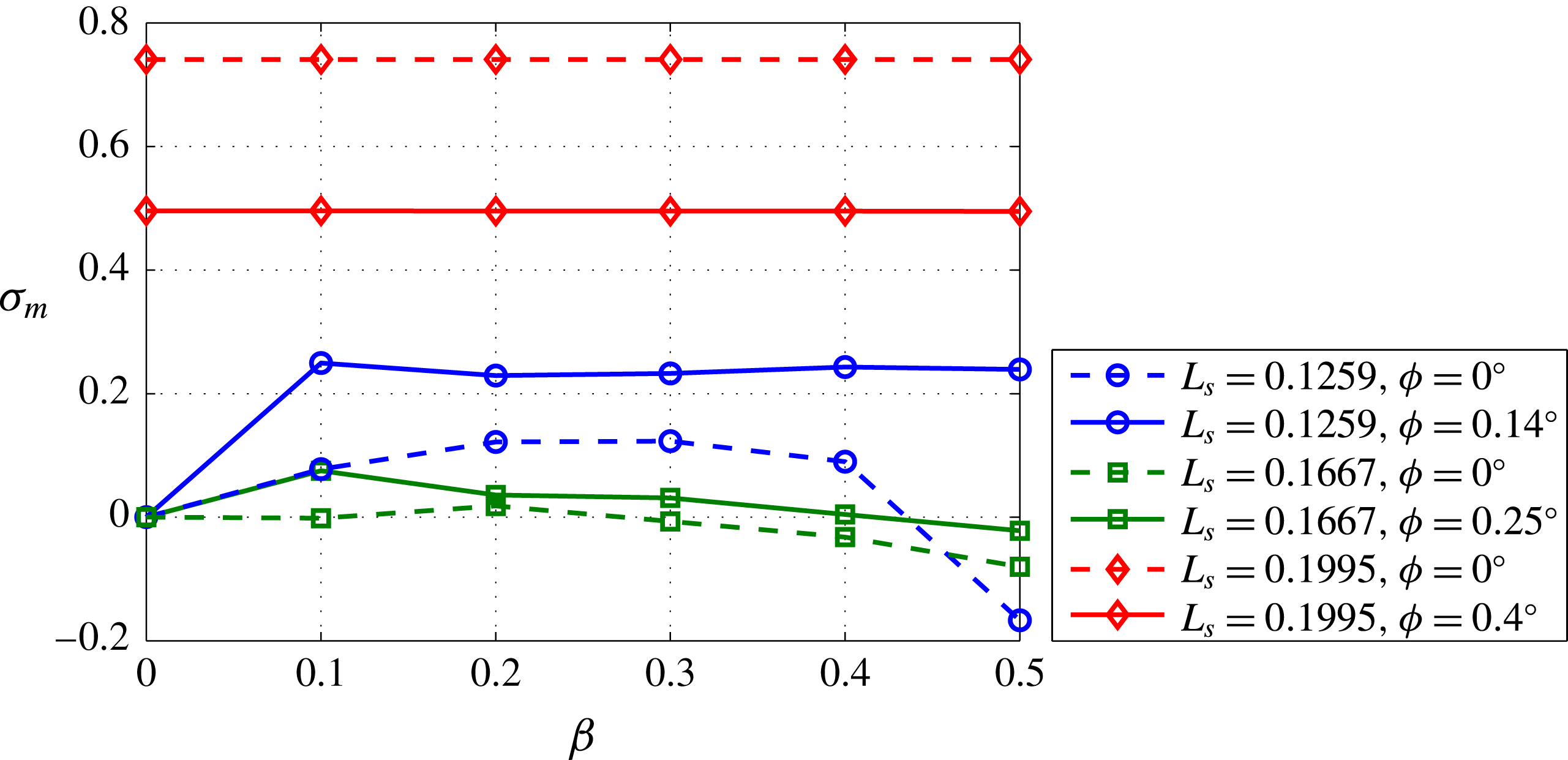
Figure 19. Secondary stability analysis of steady convective states. Variation of the maximum growth rate,
 $\unicode[STIX]{x1D70E}_{m}$
, with the Floquet parameter
$\unicode[STIX]{x1D70E}_{m}$
, with the Floquet parameter
 $\unicode[STIX]{x1D6FD}$
at
$\unicode[STIX]{x1D6FD}$
at
 $Ra=5000$
. At small
$Ra=5000$
. At small
 $L_{s}$
(e.g.
$L_{s}$
(e.g.
 $L_{s}=0.1259$
and
$L_{s}=0.1259$
and
 $0.1667$
), the base state is marginally stable for
$0.1667$
), the base state is marginally stable for
 $\unicode[STIX]{x1D6FD}=0$
, but unstable to certain long-wavelength perturbations (
$\unicode[STIX]{x1D6FD}=0$
, but unstable to certain long-wavelength perturbations (
 $0<\unicode[STIX]{x1D6FD}\leqslant 0.5$
). The inclination of the layer intensifies this long-wavelength instability. At large
$0<\unicode[STIX]{x1D6FD}\leqslant 0.5$
). The inclination of the layer intensifies this long-wavelength instability. At large
 $L_{s}$
(e.g.
$L_{s}$
(e.g.
 $L_{s}=0.1995$
), the base state is unstable even for
$L_{s}=0.1995$
), the base state is unstable even for
 $\unicode[STIX]{x1D6FD}=0$
, and the growth rate (which is associated with the wall mode) becomes independent of
$\unicode[STIX]{x1D6FD}=0$
, and the growth rate (which is associated with the wall mode) becomes independent of
 $\unicode[STIX]{x1D6FD}$
. Moreover, for
$\unicode[STIX]{x1D6FD}$
. Moreover, for
 $L_{s}=0.1995$
, this growth rate actually is reduced when the layer becomes inclined, although this is not necessarily true for even larger
$L_{s}=0.1995$
, this growth rate actually is reduced when the layer becomes inclined, although this is not necessarily true for even larger
 $L_{s}$
.
$L_{s}$
.
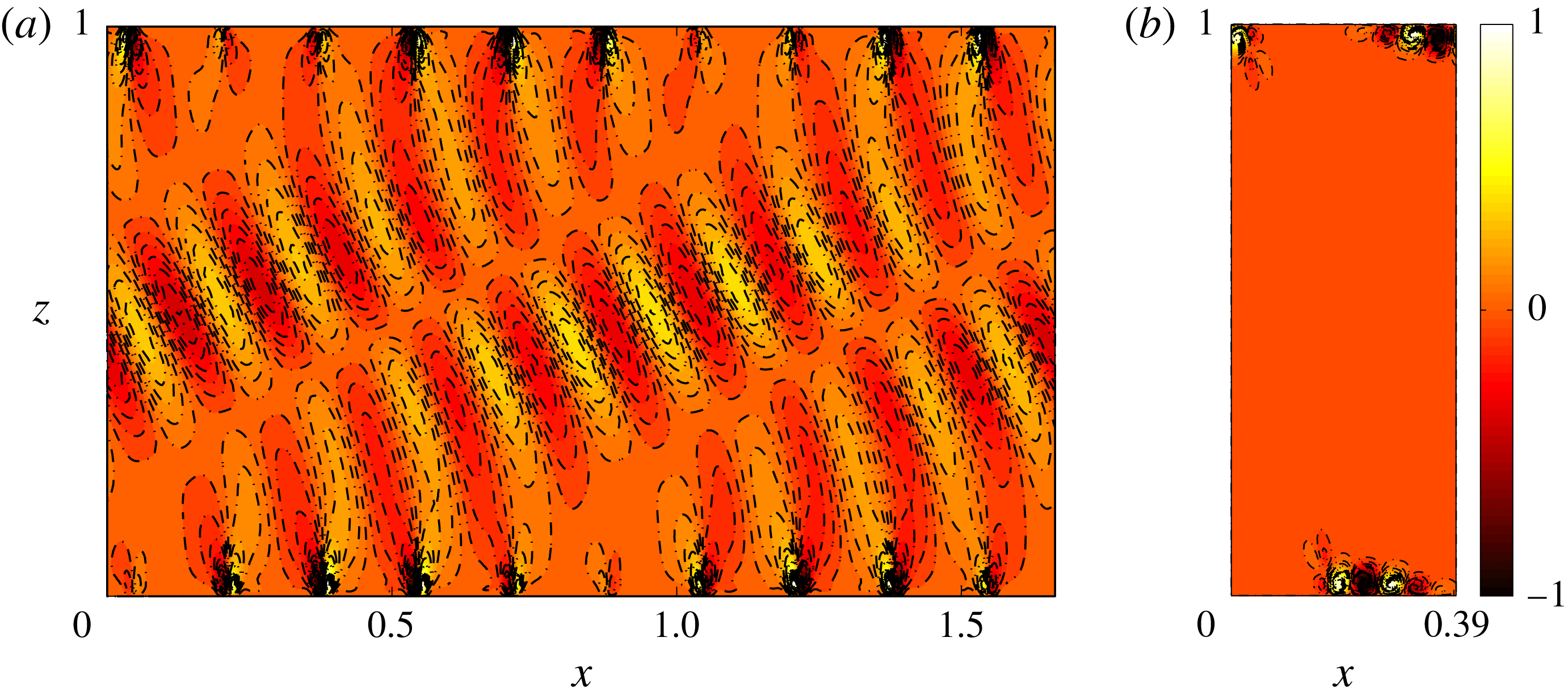
Figure 20. The fastest-growing 2D temperature eigenfunction at
 $Ra=5000$
in inclined PMC: (a)
$Ra=5000$
in inclined PMC: (a)
 $L_{s}=0.1667$
,
$L_{s}=0.1667$
,
 $\unicode[STIX]{x1D719}=0.25^{\circ }$
,
$\unicode[STIX]{x1D719}=0.25^{\circ }$
,
 $\unicode[STIX]{x1D6FD}=0.1$
; (b)
$\unicode[STIX]{x1D6FD}=0.1$
; (b)
 $L_{s}=0.3981$
,
$L_{s}=0.3981$
,
 $\unicode[STIX]{x1D719}=6^{\circ }$
,
$\unicode[STIX]{x1D719}=6^{\circ }$
,
 $\unicode[STIX]{x1D6FD}=0$
. The eigenfunctions in panel (a) are shown in a domain with aspect ratio
$\unicode[STIX]{x1D6FD}=0$
. The eigenfunctions in panel (a) are shown in a domain with aspect ratio
 $L=10L_{s}$
. As in the horizontal case, at small
$L=10L_{s}$
. As in the horizontal case, at small
 $L_{s}$
(a), a bulk mode controls the instability, and at large
$L_{s}$
(a), a bulk mode controls the instability, and at large
 $L_{s}$
(b), a wall mode dominates. In the latter case, note that the instability is further localised within the antinatural roll.
$L_{s}$
(b), a wall mode dominates. In the latter case, note that the instability is further localised within the antinatural roll.
At large
 $Ra$
, the steady state for the inclined case exhibits similar instability properties as for the horizontal case. As shown in figure 19, at small
$Ra$
, the steady state for the inclined case exhibits similar instability properties as for the horizontal case. As shown in figure 19, at small
 $L_{s}$
, the steady states for both the horizontal and inclined porous layers are unstable for a range of long-wavelength perturbations (
$L_{s}$
, the steady states for both the horizontal and inclined porous layers are unstable for a range of long-wavelength perturbations (
 $0<\unicode[STIX]{x1D6FD}\leqslant 0.5$
), and this type of instability is enhanced in the inclined case. However, at large
$0<\unicode[STIX]{x1D6FD}\leqslant 0.5$
), and this type of instability is enhanced in the inclined case. However, at large
 $L_{s}$
, the maximum growth rate
$L_{s}$
, the maximum growth rate
 $\unicode[STIX]{x1D70E}_{m}\equiv \text{Re}\unicode[STIX]{x1D706}_{m}^{\star }/Ra$
for both the horizontal and inclined cases becomes independent of
$\unicode[STIX]{x1D70E}_{m}\equiv \text{Re}\unicode[STIX]{x1D706}_{m}^{\star }/Ra$
for both the horizontal and inclined cases becomes independent of
 $\unicode[STIX]{x1D6FD}$
. Figure 20 shows the 2D eigenfunctions corresponding to these two families of secondary instabilities. As in the horizontal case, at small
$\unicode[STIX]{x1D6FD}$
. Figure 20 shows the 2D eigenfunctions corresponding to these two families of secondary instabilities. As in the horizontal case, at small
 $L_{s}$
, e.g.
$L_{s}$
, e.g.
 $L_{s}=0.1667$
, when the growth rate depends on the wall-parallel wavenumber
$L_{s}=0.1667$
, when the growth rate depends on the wall-parallel wavenumber
 $\unicode[STIX]{x1D6FD}k_{s}$
, the most unstable perturbation is a bulk mode that spans the layer (figure 20
a). However, at large
$\unicode[STIX]{x1D6FD}k_{s}$
, the most unstable perturbation is a bulk mode that spans the layer (figure 20
a). However, at large
 $L_{s}$
, e.g.
$L_{s}$
, e.g.
 $L_{s}=0.3981$
, when the growth rate is independent of
$L_{s}=0.3981$
, when the growth rate is independent of
 $\unicode[STIX]{x1D6FD}$
, the most unstable perturbation for each
$\unicode[STIX]{x1D6FD}$
, the most unstable perturbation for each
 $\unicode[STIX]{x1D6FD}$
is a wall mode that is strongly localised near the upper and lower walls (figure 20
b). Moreover, the wall mode has a very similar spatial structure for each
$\unicode[STIX]{x1D6FD}$
is a wall mode that is strongly localised near the upper and lower walls (figure 20
b). Moreover, the wall mode has a very similar spatial structure for each
 $\unicode[STIX]{x1D6FD}$
, as in the horizontal case. Crucially, when
$\unicode[STIX]{x1D6FD}$
, as in the horizontal case. Crucially, when
 $\unicode[STIX]{x1D719}$
is sufficiently large, the fastest-growing wall mode only occurs in the antinatural roll (see figure 20
b), confirming that the antinatural roll is more unstable than the natural roll.
$\unicode[STIX]{x1D719}$
is sufficiently large, the fastest-growing wall mode only occurs in the antinatural roll (see figure 20
b), confirming that the antinatural roll is more unstable than the natural roll.
5.3 Nonlinear evolution of the instability
In horizontal PMC, two types of instability have been found at large
 $Ra$
: a bulk-mode instability in which narrow plumes merge to form wider ones; and a wall-mode instability that splits the wide plumes, creating narrower ones (Wen et al.
Reference Wen, Corson and Chini2015b
). In the inclined case, DNS indicate that unsteady narrow plumes in the domain interior undergo merging events to form a metastable pattern consisting of more widely spaced plumes (see figure 9). To gain insight into the mechanics of this process, strategically initialised DNS were performed to investigate the nonlinear evolution of the fastest-growing secondary instability mode. Initial conditions were generated by first replicating the steady state at a given
$Ra$
: a bulk-mode instability in which narrow plumes merge to form wider ones; and a wall-mode instability that splits the wide plumes, creating narrower ones (Wen et al.
Reference Wen, Corson and Chini2015b
). In the inclined case, DNS indicate that unsteady narrow plumes in the domain interior undergo merging events to form a metastable pattern consisting of more widely spaced plumes (see figure 9). To gain insight into the mechanics of this process, strategically initialised DNS were performed to investigate the nonlinear evolution of the fastest-growing secondary instability mode. Initial conditions were generated by first replicating the steady state at a given
 $L_{s}$
in a wider domain and then superposing a small-amplitude contribution of the most unstable secondary instability mode in the spatially extended domain.
$L_{s}$
in a wider domain and then superposing a small-amplitude contribution of the most unstable secondary instability mode in the spatially extended domain.
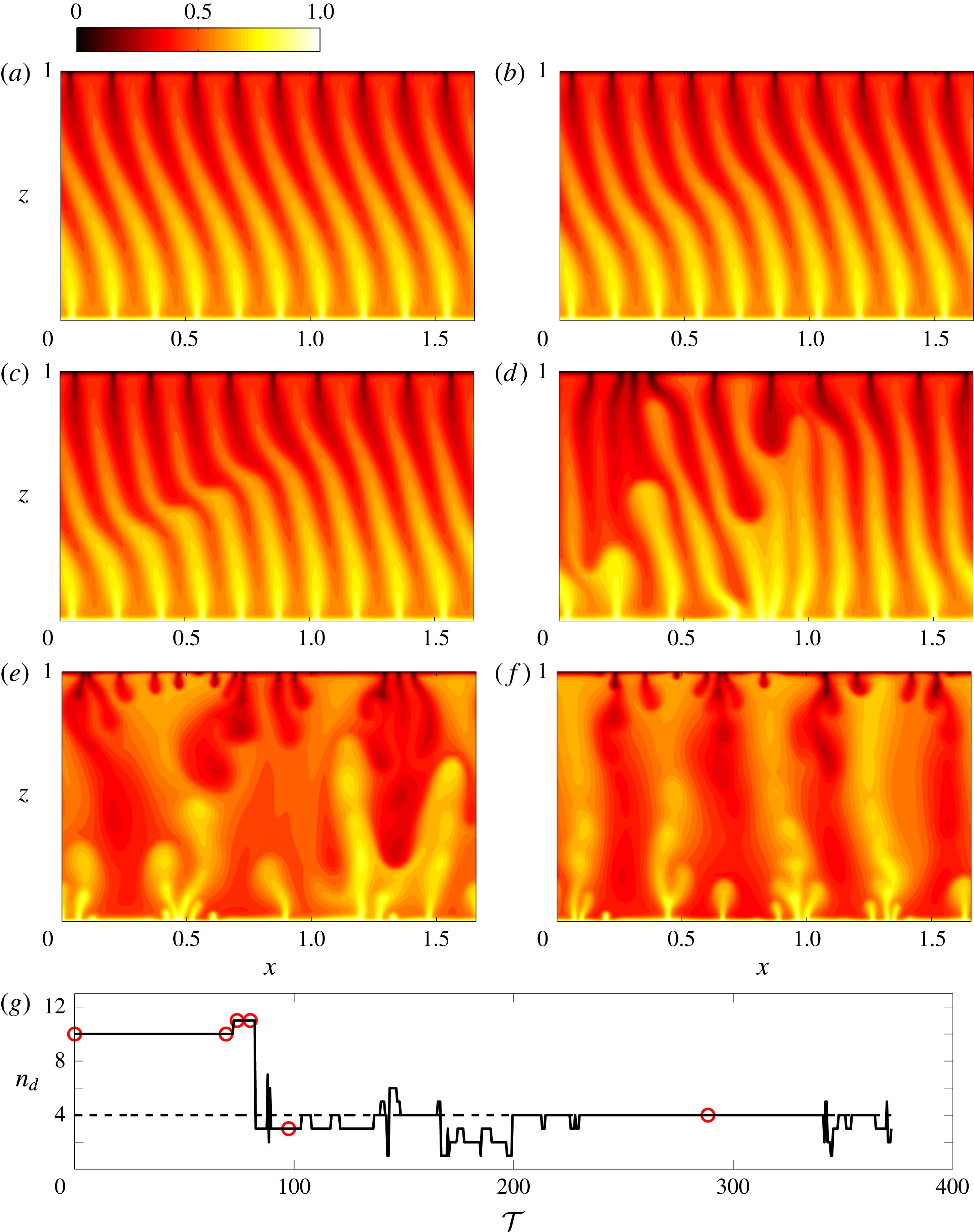
Figure 21. Snapshots of temperature fields extracted from DNS showing the nonlinear evolution of the fastest-growing secondary instability mode for
 $L_{s}=0.1667$
,
$L_{s}=0.1667$
,
 $\unicode[STIX]{x1D6FD}=0.1$
,
$\unicode[STIX]{x1D6FD}=0.1$
,
 $L=10L_{s}$
,
$L=10L_{s}$
,
 $Ra=5000$
,
$Ra=5000$
,
 $\unicode[STIX]{x1D719}=0.25^{\circ }$
: (a)
$\unicode[STIX]{x1D719}=0.25^{\circ }$
: (a)
 ${\mathcal{T}}=0$
; (b)
${\mathcal{T}}=0$
; (b)
 ${\mathcal{T}}=69$
; (c)
${\mathcal{T}}=69$
; (c)
 ${\mathcal{T}}=74$
; (d)
${\mathcal{T}}=74$
; (d)
 ${\mathcal{T}}=80$
; (e)
${\mathcal{T}}=80$
; (e)
 ${\mathcal{T}}=97.5$
; (f)
${\mathcal{T}}=97.5$
; (f)
 ${\mathcal{T}}=288.5$
. (g) The time evolution of the dominant wall-parallel mode number
${\mathcal{T}}=288.5$
. (g) The time evolution of the dominant wall-parallel mode number
 $n_{d}$
at
$n_{d}$
at
 $z=0.5$
(solid line). The dashed line shows the time-mean dominant mode number and the circles correspond to the times highlighted in panels (a–f).
$z=0.5$
(solid line). The dashed line shows the time-mean dominant mode number and the circles correspond to the times highlighted in panels (a–f).
Figure 21 shows the nonlinear evolution of the fastest-growing secondary instability mode for small
 $L_{s}$
within the bulk instability parameter regime. The initial condition comprises
$L_{s}$
within the bulk instability parameter regime. The initial condition comprises
 $10$
replicas of the steady convective state at
$10$
replicas of the steady convective state at
 $L_{s}=0.1667$
plus a small-amplitude contribution of the corresponding fastest-growing perturbation at
$L_{s}=0.1667$
plus a small-amplitude contribution of the corresponding fastest-growing perturbation at
 $\unicode[STIX]{x1D6FD}=0.1$
(see figure 20
a). In accord with the predictions of the secondary stability analysis, and as is evident in figure 21(b,c), the steady convective base state is unstable to a bulk mode in this case. As the secondary mode grows in amplitude, some narrow plumes become so distorted that the cold (heavy) plumes then overlie the hot (light) ones (see figure 21
c). These strongly distorted plumes then break down and merge to form wider plumes, as shown in figure 21(d,e). The resulting widely spaced plumes, however, are strongly unstable to a wall-mode instability: some plumes growing from the upper and lower boundary layers split the wider plumes, creating narrower ones (see figure 21
e,f). Interestingly, this process, i.e. distorted narrow columnar flow
$\unicode[STIX]{x1D6FD}=0.1$
(see figure 20
a). In accord with the predictions of the secondary stability analysis, and as is evident in figure 21(b,c), the steady convective base state is unstable to a bulk mode in this case. As the secondary mode grows in amplitude, some narrow plumes become so distorted that the cold (heavy) plumes then overlie the hot (light) ones (see figure 21
c). These strongly distorted plumes then break down and merge to form wider plumes, as shown in figure 21(d,e). The resulting widely spaced plumes, however, are strongly unstable to a wall-mode instability: some plumes growing from the upper and lower boundary layers split the wider plumes, creating narrower ones (see figure 21
e,f). Interestingly, this process, i.e. distorted narrow columnar flow
 $\rightarrow$
bulk instability
$\rightarrow$
bulk instability
 $\rightarrow$
wider columnar flow, agrees very well with the phenomenon observed in DNS for columnar flows (see figure 9). Therefore, in the inclined porous layer, the bulk-mode instability enhances the distortion of narrowly spaced plumes, causing plume merger and coarsening the convective pattern.
$\rightarrow$
wider columnar flow, agrees very well with the phenomenon observed in DNS for columnar flows (see figure 9). Therefore, in the inclined porous layer, the bulk-mode instability enhances the distortion of narrowly spaced plumes, causing plume merger and coarsening the convective pattern.
6 Conclusion
DNS and stability and variational upper-bound analyses have been performed to investigate pattern formation in and the transport properties of high-
 $Ra$
convection in a 2D inclined porous layer uniformly heated from the below and cooled from above. As expected, the DNS confirm that the base shear flow induced by the inclination of the porous layer significantly impacts the flow structure and heat transport at large values of the Rayleigh number. For
$Ra$
convection in a 2D inclined porous layer uniformly heated from the below and cooled from above. As expected, the DNS confirm that the base shear flow induced by the inclination of the porous layer significantly impacts the flow structure and heat transport at large values of the Rayleigh number. For
 $0^{\circ }<\unicode[STIX]{x1D719}\lesssim 25^{\circ }$
, the flow exhibits a three-region wall-normal columnar structure as in the horizontal case, except that as
$0^{\circ }<\unicode[STIX]{x1D719}\lesssim 25^{\circ }$
, the flow exhibits a three-region wall-normal columnar structure as in the horizontal case, except that as
 $\unicode[STIX]{x1D719}$
is increased the time-mean interplume spacing also is substantially increased. Nevertheless, for
$\unicode[STIX]{x1D719}$
is increased the time-mean interplume spacing also is substantially increased. Nevertheless, for
 $0^{\circ }<\unicode[STIX]{x1D719}\lesssim 20^{\circ }$
, the Nusselt number is little affected by the inclination of the layer. As the inclination angle is increased, however, the background mean shear flow strengthens, thereby intensifying the natural-roll motions and suppressing the antinatural-roll motions. Consequently, when
$0^{\circ }<\unicode[STIX]{x1D719}\lesssim 20^{\circ }$
, the Nusselt number is little affected by the inclination of the layer. As the inclination angle is increased, however, the background mean shear flow strengthens, thereby intensifying the natural-roll motions and suppressing the antinatural-roll motions. Consequently, when
 $\unicode[STIX]{x1D719}>\unicode[STIX]{x1D719}_{t}$
, where
$\unicode[STIX]{x1D719}>\unicode[STIX]{x1D719}_{t}$
, where
 $30^{\circ }<\unicode[STIX]{x1D719}_{t}<32^{\circ }$
independently of
$30^{\circ }<\unicode[STIX]{x1D719}_{t}<32^{\circ }$
independently of
 $Ra$
, the antinatural rolls become detached from the upper and lower walls and the columnar flow structure is completely broken down: the flow transitions to a large-scale travelling-wave convective roll state, and the heat transport is significantly reduced.
$Ra$
, the antinatural rolls become detached from the upper and lower walls and the columnar flow structure is completely broken down: the flow transitions to a large-scale travelling-wave convective roll state, and the heat transport is significantly reduced.
Interestingly, our results show that the transition angle
 $\unicode[STIX]{x1D719}_{t}$
from columnar flow to convective travelling-wave states observed in the DNS can be well predicted by the linear stability analysis, i.e.
$\unicode[STIX]{x1D719}_{t}$
from columnar flow to convective travelling-wave states observed in the DNS can be well predicted by the linear stability analysis, i.e.
 $\unicode[STIX]{x1D719}_{t}\approx 31.3^{\circ }$
, above which the basic state is linearly stable to 2D disturbances independently of
$\unicode[STIX]{x1D719}_{t}\approx 31.3^{\circ }$
, above which the basic state is linearly stable to 2D disturbances independently of
 $Ra$
(Rees & Bassom Reference Rees and Bassom2000). Our energy stability analysis, however, indicates that at large
$Ra$
(Rees & Bassom Reference Rees and Bassom2000). Our energy stability analysis, however, indicates that at large
 $Ra$
the basic state is not nonlinearly stable for any
$Ra$
the basic state is not nonlinearly stable for any
 $\unicode[STIX]{x1D719}<90^{\circ }$
, confirming that convective states may be realisable. Moreover, the upper-bound analysis shows that for
$\unicode[STIX]{x1D719}<90^{\circ }$
, confirming that convective states may be realisable. Moreover, the upper-bound analysis shows that for
 $0^{\circ }<\unicode[STIX]{x1D719}\leqslant 90^{\circ }$
,
$0^{\circ }<\unicode[STIX]{x1D719}\leqslant 90^{\circ }$
,
 $Nu\sim CRa$
with a prefactor
$Nu\sim CRa$
with a prefactor
 $C$
that monotonically decreases as
$C$
that monotonically decreases as
 $\unicode[STIX]{x1D719}$
is increased. Neither the energy stability theory nor the CDH upper-bound analysis predicts the transition angle observed in the DNS, since a gap in the parameter values for linear and nonlinear stability of the basic state is required for this transition. This gap implies the possibility of a subcritical bifurcation, which may give rise to spatially localised convective states. Indeed, for
$\unicode[STIX]{x1D719}$
is increased. Neither the energy stability theory nor the CDH upper-bound analysis predicts the transition angle observed in the DNS, since a gap in the parameter values for linear and nonlinear stability of the basic state is required for this transition. This gap implies the possibility of a subcritical bifurcation, which may give rise to spatially localised convective states. Indeed, for
 $\unicode[STIX]{x1D719}>\unicode[STIX]{x1D719}_{t}$
and more moderate values of
$\unicode[STIX]{x1D719}>\unicode[STIX]{x1D719}_{t}$
and more moderate values of
 $Ra$
, not only have we observed localised convective states in our DNS (Wen Reference Wen2015) but we also have succeeded in isolating them in our fully nonlinear steady-state computations. Nevertheless, we defer a more thorough investigation and analysis of these spatially localised solutions to a future study.
$Ra$
, not only have we observed localised convective states in our DNS (Wen Reference Wen2015) but we also have succeeded in isolating them in our fully nonlinear steady-state computations. Nevertheless, we defer a more thorough investigation and analysis of these spatially localised solutions to a future study.
To better understand the physics of inclined porous medium convection at modest
 $\unicode[STIX]{x1D719}$
, the structure and stability of steady nonlinear convective states were investigated at large
$\unicode[STIX]{x1D719}$
, the structure and stability of steady nonlinear convective states were investigated at large
 $Ra$
. Our solutions reveal that fully nonlinear steady convective states with disparate aspect ratios are distorted differently; specifically, the narrow steady states are distorted in a counterclockwise sense, as also is observed in DNS when the plumes are narrowly spaced. The linear stability analysis of these (2D) steady convective flows reveals that two types of instability exist when
$Ra$
. Our solutions reveal that fully nonlinear steady convective states with disparate aspect ratios are distorted differently; specifically, the narrow steady states are distorted in a counterclockwise sense, as also is observed in DNS when the plumes are narrowly spaced. The linear stability analysis of these (2D) steady convective flows reveals that two types of instability exist when
 $\unicode[STIX]{x1D719}\neq 0^{\circ }$
: a bulk-mode instability and a wall-mode instability, consistent with previous findings for
$\unicode[STIX]{x1D719}\neq 0^{\circ }$
: a bulk-mode instability and a wall-mode instability, consistent with previous findings for
 $\unicode[STIX]{x1D719}=0^{\circ }$
. Importantly, the nonlinear evolution of the most unstable mode for the narrow steady states suggests that the instability process observed in DNS for narrow columnar flows (see figure 9) corresponds to a bulk-mode instability, which is intensified by the inclination of the layer, thereby favouring increased spacing between the interior plumes relative to the
$\unicode[STIX]{x1D719}=0^{\circ }$
. Importantly, the nonlinear evolution of the most unstable mode for the narrow steady states suggests that the instability process observed in DNS for narrow columnar flows (see figure 9) corresponds to a bulk-mode instability, which is intensified by the inclination of the layer, thereby favouring increased spacing between the interior plumes relative to the
 $\unicode[STIX]{x1D719}=0^{\circ }$
scenario. Finally, we remark that although our study has focused on 2D PMC in a laterally periodic domain, DNS by Pau et al. (Reference Pau, Bell, Pruess, Almgren, Lijewski and Zhang2010), Fu, Cueto-Felgueroso & Juanes (Reference Fu, Cueto-Felgueroso and Juanes2013) and Hewitt, Neufeld & Lister (Reference Hewitt, Neufeld and Lister2014) indicate that the flow in a 3D horizontal porous layer at large
$\unicode[STIX]{x1D719}=0^{\circ }$
scenario. Finally, we remark that although our study has focused on 2D PMC in a laterally periodic domain, DNS by Pau et al. (Reference Pau, Bell, Pruess, Almgren, Lijewski and Zhang2010), Fu, Cueto-Felgueroso & Juanes (Reference Fu, Cueto-Felgueroso and Juanes2013) and Hewitt, Neufeld & Lister (Reference Hewitt, Neufeld and Lister2014) indicate that the flow in a 3D horizontal porous layer at large
 $Ra$
also exhibits a three-region asymptotic columnar structure, suggesting that polyhedral cells at small inclination angles probably have a columnar structure at large
$Ra$
also exhibits a three-region asymptotic columnar structure, suggesting that polyhedral cells at small inclination angles probably have a columnar structure at large
 $Ra$
. Moreover, the investigation by Voss et al. (Reference Voss, Simmons and Robinson2010) suggests that the effect of sidewalls is negligible for domains with aspect ratios
$Ra$
. Moreover, the investigation by Voss et al. (Reference Voss, Simmons and Robinson2010) suggests that the effect of sidewalls is negligible for domains with aspect ratios
 $L\gtrsim 10$
. Therefore, our 2D investigation may provide at least partial insight into the physics of 3D inclined porous medium convection in bounded but sufficiently wide domains.
$L\gtrsim 10$
. Therefore, our 2D investigation may provide at least partial insight into the physics of 3D inclined porous medium convection in bounded but sufficiently wide domains.
Acknowledgements
We thank C. Doering and R. Kerswell for helpful discussions. This work was in part funded by an ICES postdoctoral fellowship held by B.W. at the University of Texas at Austin and by NSF Award DMS-0928098 (G.P.C.). This work was also supported as part of the Center for Frontiers of Subsurface Energy Security, an Energy Frontier Research Center funded by the U.S. Department of Energy, Office of Science, Basic Energy Sciences under Award no. DE-SC0001114.


