


1 Introduction
In wall flows, the study of large-scale coherent structures has received particular attention because such structures carry a large portion of the turbulent kinetic energy and contribute significantly to the transport of momentum and relevant scalars such as heat, oxygen and pollutants (Robinson Reference Robinson1991; Marusic et al. Reference Marusic, McKeon, Monkewitz, Nagib, Smits and Sreenivasan2010; Jiménez Reference Jiménez2018). There is now compelling evidence that, in canonical smooth-wall flows – which include (flat-plate) turbulent boundary layers, closed-channel and pipe flows – two distinct large-scale structures occur, which are commonly referred to as large-scale motions (LSMs) and very-large-scale motions (VLSMs). While there are several methods to visualise and identify such structures, the most employed diagnostic tool is based on pre-multiplied one-dimensional (1-D) spectra, where LSMs and VLSMs impose two well-defined peaks (Kim & Adrian Reference Kim and Adrian1999; Hutchins & Marusic Reference Hutchins and Marusic2007b). Many studies have proven that such peaks occur at wavenumbers that scale with the characteristic outer length scale of the flow  $\unicode[STIX]{x1D6FF}$ (Kim & Adrian Reference Kim and Adrian1999; Adrian, Meinhart & Tomkins Reference Adrian, Meinhart and Tomkins2000; Del Álamo & Jiménez Reference Del Álamo and Jiménez2003; Ganapathisubramani, Longmire & Marusic Reference Ganapathisubramani, Longmire and Marusic2003; Tomkins & Adrian Reference Tomkins and Adrian2003; Hutchins, Hambleton & Marusic Reference Hutchins, Hambleton and Marusic2005; Guala, Hommema & Adrian Reference Guala, Hommema and Adrian2006; Balakumar & Adrian Reference Balakumar and Adrian2007; Hutchins & Marusic Reference Hutchins and Marusic2007a,Reference Hutchins and Marusicb; Monty et al. Reference Monty, Stewart, Williams and Chong2007, Reference Monty, Hutchins, Ng, Marusic and Chong2009; Sillero, Jiménez & Moser Reference Sillero, Jiménez and Moser2014; De Silva et al. Reference De Silva, Kevin, Baidya, Hutchins and Marusic2018).
In order to obtain a clear distinction between the two aforementioned peaks, though, Hutchins & Marusic (Reference Hutchins and Marusic2007b) recommend that the von Kármán number  $Re_{\unicode[STIX]{x1D70F}}=\unicode[STIX]{x1D6FF}u_{\unicode[STIX]{x1D70F}}/\unicode[STIX]{x1D708}$ (where
  $u_{\unicode[STIX]{x1D70F}}$ is the shear velocity and
  $\unicode[STIX]{x1D708}$ is the kinematic viscosity) of the flow should not be less than 1700. This number is a reference value that ensures one order of magnitude of length-scale separation between LSMs and VLSMs in turbulent boundary layers. When this condition is satisfied, Hutchins & Marusic (Reference Hutchins and Marusic2007a,Reference Hutchins and Marusicb) showed that wavenumbers associated with LSM and VLSM peaks correspond to structures whose longitudinal size is
  $(2{-}3)\unicode[STIX]{x1D6FF}$ and
  $6\unicode[STIX]{x1D6FF}$, respectively. It was also observed that LSM peaks persist throughout most of the outer layer while VLSM peaks vanish above the logarithmic region.
As far as pipe and channel flows are concerned, the picture is significantly different from boundary layers because spectral peaks corresponding to VLSMs are detectable well within the outer layer (Monty et al. Reference Monty, Stewart, Williams and Chong2007, Reference Monty, Hutchins, Ng, Marusic and Chong2009; Sillero et al. Reference Sillero, Jiménez and Moser2014) and correspond to scales up to  $20\unicode[STIX]{x1D6FF}$. More similarly to turbulent boundary layers, LSM peaks were observed to scale as
  $3\unicode[STIX]{x1D6FF}$ and to persist up to the channel/pipe centreline (see also Kim & Adrian Reference Kim and Adrian1999; Guala et al. Reference Guala, Hommema and Adrian2006; Balakumar & Adrian Reference Balakumar and Adrian2007).
Regarding the generation mechanism of LSMs and VLSMs, the literature proposes two potential explanations associated with two approaches. There is a so-called ‘parent–offspring’ approach whereby LSMs are considered to emerge out of the alignment of hairpin-vortex packets and VLSMs, in turn, as groups of aligned LSM packets (Hommema & Adrian Reference Hommema and Adrian2002; Adrian Reference Adrian2007; Adrian & Marusic Reference Adrian and Marusic2012; Katul Reference Katul2019). The second approach, instead, claims that VLSMs and LSMs are a direct consequence of a mean-flow instability process and their existence is independent of the dynamics of smaller-scale structures, such as hairpin vortices, which, in the first approach, are instead considered as the building block of wall turbulence (Hwang & Cossu Reference Hwang and Cossu2010). In the second approach, given their streaky and meandering nature and their marked longitudinal vorticity, VLSMs are interpreted to be the principal actors of a self-sustaining ‘outer-layer’ cycle, which shares analogies with its better understood near-wall (i.e. in the buffer layer) counterpart, where VLSMs play the same role as the so-called elongated streamwise vortices (Rawat et al. Reference Rawat, Cossu, Hwang and Rincon2015; Hwang & Bengana Reference Hwang and Bengana2016; Hwang, Willis & Cossu Reference Hwang, Willis and Cossu2016; Cossu & Hwang Reference Cossu and Hwang2017).
Large-scale coherent structures have been extensively studied also in open-channel flows, which are the subject of the present study, as they influence ecologically relevant scalar transport processes (such as oxygen, nutrients and sediments), river morphodynamics and even the power output of hydro-kinetic marine turbines (Moog & Jirka Reference Moog and Jirka1999; Jirka, Herlina & Niepelt Reference Jirka, Herlina and Niepelt2010; Nepf Reference Nepf2012; Venditti et al. Reference Venditti, Best, Church and Hardy2013; Chamorro et al. Reference Chamorro, Hill, Morton, Ellis, Arndt and Sotiropoulos2013; Trinci et al. Reference Trinci, Harvey, Henshaw, Bertoldi and Hölker2017; Cameron, Nikora & Marusic Reference Cameron, Nikora and Marusic2019). Laboratory and field experiments have detected the presence of large-scale wedge-type structures, whose sizes in the streamwise, spanwise and wall-normal directions are expressed as a function of the outer scale, namely, the water depth  $h$ (Jackson Reference Jackson1976; Nakagawa & Nezu Reference Nakagawa and Nezu1981; Rashidi & Banerjee Reference Rashidi and Banerjee1988; Nezu & Nakagawa Reference Nezu and Nakagawa1993; Rashidi Reference Rashidi1997; Shen & Lemmin Reference Shen and Lemmin1999; Tamburrino & Gulliver Reference Tamburrino and Gulliver1999; Shvidchenko & Pender Reference Shvidchenko and Pender2001; Cellino & Lemmin Reference Cellino and Lemmin2004; Roy et al. Reference Roy, Buffin-Belanger, Lamarre and Kirkbride2004; Hurther, Lemmin & Terray Reference Hurther, Lemmin and Terray2007; Franca & Lemmin Reference Franca and Lemmin2015; Zhong et al. Reference Zhong, Chen, Wang, Li and Wang2016; Da Silva & Yalin Reference Da Silva and Yalin2017; Bagherimiyab & Lemmin Reference Bagherimiyab and Lemmin2018; Ghesemi, Fox & Husic Reference Ghesemi, Fox and Husic2019).
Although some studies indicate the presence of long structures with streamwise vorticity, which resemble the VLSMs as defined in canonical flows (Grinvald & Nikora Reference Grinvald and Nikora1988; Nezu Reference Nezu2005; Sukhodolov, Nikora & Katolikov Reference Sukhodolov, Nikora and Katolikov2011; Zhong et al. Reference Zhong, Li, Chen and Wang2015), Cameron, Nikora & Stewart (Reference Cameron, Nikora and Stewart2017) were the first to provide insights into the occurrence and scaling of VLSMs in turbulent open-channel flows. In that study, the authors present long-duration particle image velocimetry measurements in fully rough open-channel flows over a bed made of spheres packed in a hexagonal arrangement. Among the numerous results, they report pre-multiplied spectra of the longitudinal velocity component, which display the characteristic double-peak behaviour observed for canonical wall flows. They also report that one of the peaks occurs at wavelengths of approximately  $6{-}7h$ and nicely scales with the water depth. This peak was associated with the presence of LSMs. The other peak occurred at wavelengths consistent with those pertaining to VLSMs, but not scaling with the flow depth. Moreover, such wavelengths were recorded to be up to 50 times the water depth
  $h$. If
  $h$ is taken as the representative outer length scale (as is normally assumed), this means that the non-dimensional length of VLSMs in open-channel flows (as detected from pre-multiplied spectral peaks) is much greater than in other canonical wall flows. Owing to the mismatch between the VLSM and LSM scaling, the authors concluded that, in open-channel flows, these two types of structures might be generated by independent and, possibly, different mechanisms.
Unfortunately, owing to the fact that the experiments were performed in rough-wall conditions, Cameron et al. (Reference Cameron, Nikora and Stewart2017) could not unambiguously identify the non-dimensional parameter controlling the scaling of VLSMs among the following: the aspect ratio  $W/h$, the relative submergence
  $h/D$ and the von Kármán number
  $Re_{\unicode[STIX]{x1D70F}}$ (where
  $W$ is the channel width and
  $D$ is the diameter of the spheres). The number of factors further increased when, in a subsequent study, the same authors (Cameron et al. Reference Cameron, Nikora, Stewart and Zampiron2018) noticed that VLSM wavelengths were also dependent on the non-dimensional distance from the flume inlet
  $x/h$. Despite the large number of parameters involved, Cameron et al. (Reference Cameron, Nikora and Stewart2017) argued that the aspect ratio
  $W/h$ was the most plausible ‘culprit’ for the variation of depth-normalised VLSM wavelengths. The authors justify this hypothesis on the basis that VLSMs and
  $W$ are of the same order of magnitude and hence
  $W$ might constrain the growth of VLSMs.
The main aim of the present work is to further explore the scaling of LSMs and VLSMs in open-channel flows. Towards this end, we present results from a series of smooth-bed experiments, as they are free from complicating factors associated with rough beds. In fact, in smooth-bed open-channel flows, the number of non-dimensional parameters that may influence the scaling of large-scale structures reduces from four to three, namely  $Re_{\unicode[STIX]{x1D70F}}$,
  $W/h$ and
  $x/h$. It should be emphasised that the experiments reported herein were carried out in non-uniform flow conditions, which can represent a potential complicating factor. As extensively discussed in the next section, though, non-uniformity levels were kept mild and constrained within a limited range. Besides guaranteeing that self-similar flow conditions would be established, this allowed for a comparative analysis between different tests, where the effects of
  $Re_{\unicode[STIX]{x1D70F}}$,
  $W/h$ and
  $x/h$ on velocity statistics (with a specific focus on velocity spectra) could be reasonably isolated and explored.
After this introduction, the present paper is structured as follows: § 2 outlines the experimental methodology; § 3 reports and describes the results coming from velocity measurements and is split into two parts, with § 3.1 presenting classical one-point velocity statistics and § 3.2 presenting and discussing the core of the results via spectral analysis; finally, § 4 is devoted to conclusions.
2 Experimental methodology
2.1 Experimental set-up

Figure 1. Overview of the flume used for the experiments: (a) sketch of the whole hydraulic circuit; (b) and (c) details of the inlet flow conditions and the test section, respectively. Panel (c) also shows the system of coordinate axes chosen in the present study (i.e. the streamwise  $x$, wall-normal
  $y$ and spanwise
  $z$ directions) and defines the flow depth
  $h$ and the channel width
  $W$. Note that the coordinate
  $x$ has its origin at the downstream end of the ramp – see panel (b).
Experiments were carried out in a large-scale, non-tilting, recirculating, open-channel flume at the Hydraulics Laboratory of the Politecnico di Torino (figure 1a). The main part of the facility is composed of a rectangular channel, which is 50 m long, 0.61 m wide and 1 m deep. The flume has glass sidewalls and a bed that is made mainly of steel and in some parts of glass. The flume bottom needed to be raised in order to allow for near-wall laser Doppler anemometry (LDA) measurements, which were carried out following the technique proposed by Poggi, Porporato & Ridolfi (Reference Poggi, Porporato and Ridolfi2002), described later. To this end, smooth concrete blocks (2 m long, 0.6 m wide and 0.1 m thick) were placed over the original bed of the flume along its entire length. The Nikuradse equivalent sand roughness  $k_{s}$ for hand-finished concrete without irregularities was estimated to be equal to 0.25 mm (in line with the tabulated values listed in Henderson (Reference Henderson1966)). In the proximity of the upstream end of the flume, the original bed and the concrete blocks were gently connected by a stainless-steel ramp (1.6 m long) designed to follow the shape of a fifth-degree polynomial (Bell & Mehta Reference Bell and Mehta1988) to avoid boundary layer separation (figure 1b).
In order to further reduce turbulence generated by the hydraulic circuit, a series of wire fine-mesh screens were placed in the sump underlying the flume inlet (figure 1b). The water depth was regulated by means of a vertical slot weir placed at the downstream end of the flume and five ultrasonic distance sensors (company Fae s.r.l., model FA 18-800/I-S) were arranged along the length of the flume in order to monitor the slope of the mean water depth (distances from the  $x$ origin of 3.1 m, 21.1 m, 27.1 m, 30.8 m and 39.8 m). Each probe emits an ultrasonic signal, which propagates with a divergence angle of
  $8^{\circ }$ and is characterised by an optimal sensing distance ranging between 10 and 80 cm from the sensor. In this specific application, each probe was positioned at 80 cm from the concrete bottom, which means that free-surface fluctuations were measured over an area of
  $0.025~\text{m}^{2}$ for a water depth of 20 cm and over an area of
  $0.039~\text{m}^{2}$ for a water depth of 5 cm. The accuracy of the measured distance is
  $\pm 1~\text{mm}$, which results to be a constant value if the gauge works inside the optimal sensing distance.
A digital thermometer (precision of  $\pm 0.2\,^{\circ }\text{C}$) was employed to monitor the temperature of the water and hence estimate its kinematic viscosity
  $\unicode[STIX]{x1D708}$, for each experiment.
A submerged pump enabled water recirculation between the channel and a large underground sump, which was connected to the inlet through a pipe with diameter 200 mm where an electromagnetic flow meter was mounted to monitor the flow rate for each experimental test (figure 1a).
As already mentioned, near-wall LDA measurements were made possible by adopting the technique developed and extensively tested by Poggi et al. (Reference Poggi, Porporato and Ridolfi2002) and subsequently utilised in many other studies (Poggi, Porporato & Ridolfi Reference Poggi, Porporato and Ridolfi2003; Poggi et al. Reference Poggi, Katul, Albertson and Ridolfi2007; Escudier, Nickson & Poole Reference Escudier, Nickson and Poole2009; Manes, Poggi & Ridolfi Reference Manes, Poggi and Ridolfi2011). This technique is very simple but effective. It involves the making of a thin vertical slot in the bed that allows for the passage of the vertical LDA laser beams (figure 1c). To this end, in the proximity of the test section, the vertical slot was created simply by leaving a 3 mm gap between two adjacent concrete blocks. The lower part of the gap was filled by consolidated sand and blocked using Teflon tape. The slot created in this way proved to be effective for the undisturbed propagation of the vertical laser beams while avoiding measurable alterations of near-wall turbulence properties (see § 3.1).
The instantaneous velocity fluctuations were measured by means of a two-dimensional LDA working in backscatter configuration. The LDA system is a Dantec Dynamics Flow Explorer DPSS working with two pairs of laser beams having a wavelength of 532 nm (green) for the longitudinal component  $(u)$ and 561 nm (yellow) for the wall-normal component
  $(v)$. The intersection between these four beams creates two ellipsoidal measurement volumes of
  $2.96\times 10^{-3}~\text{mm}^{3}$ (ellipsoidal axes
  $d_{x}=0.083~\text{mm}$,
  $d_{y}=0.082~\text{mm}$ and
  $d_{z}=0.828~\text{mm}$) and
  $2.52\times 10^{-3}~\text{mm}^{3}$ (ellipsoidal axes
  $d_{x}=0.078~\text{mm}$,
  $d_{y}=0.078~\text{mm}$ and
  $d_{z}=0.785~\text{mm}$) for the measurement of
  $u$ and
  $v$, respectively – these estimates are provided by the manufacturer on the basis of the
  $\text{e}^{-2}$ light-intensity cutoff principle (see Dantec Dynamics 2011). The maximum laser power is 300 mW for each pair of laser beams. Signal processing was carried out with two Dantec Dynamics Burst Spectrum Analyzers (BSA F600-2D) and dedicated Dantec software (BSA Flow Software v6.5) set up on a local PC network station. Data were always acquired in coincidence mode to allow for the estimation of the Reynolds shear stresses. The sampling frequency
  $f_{s}$ was always between 100 Hz and 400 Hz (depending on the hydraulic conditions) and more than 500 000 velocity measurements were collected for each measurement point over a minimum duration of 40 min. This amount of data ensured a negligible sampling error for all the statistics presented in § 3.1 (i.e. the sampling error as a result is much smaller than the size of the marker symbols used in the plots). The LDA optics (Dantec Dynamics 2011) was traversed by means of a three-dimensional computer-controlled Dantec Dynamics traversing system (ISEL iMC-S8 Traverse), which allows for movements along three directions with a resolution of
  $6~\unicode[STIX]{x03BC}\text{m}$.
For each experiment, particular attention was dedicated to ensure that the LDA beams were perfectly aligned with the horizontal and vertical (i.e. gravity) directions. To this end, the flume was filled with water in quiescent conditions (this was possible by sealing the outlet of the flume with a steel cap) so that the resulting free surface could be used as a perfectly horizontal plane, which was then used as a reference for the alignment of the four laser beams. The origin of the vertical coordinates was identified by means of a sharp point gauge connected to a vernier calliper (accuracy of 0.05 mm) and left at a known distance from the bed. The LDA sampling volume was then moved towards the pointer and the backscatter signal monitored with the BSA Flow Software. While gently approaching the sampling volume towards the pointer, the backscatter signal was monitored, and when it began to be disturbed by the pointer, it was assumed that the pointer and the LDA sampling volume coincided and the elevation above the bed was recorded as a reference to identify the origin of the vertical axis. By repeating this method for multiple heights above the bed, it was observed that the zero reference level could be detected with an accuracy of approximately  $\pm 0.1~\text{mm}$ (in wall units, this uncertainty varies according to the test, with an average value of
  $\pm 1.5$).
Table 1. Summary of experiments and associated hydraulic conditions. The columns indicate: the water depth  $h$; the bulk velocity
  $U_{b}$; the shear velocity
  $u_{\unicode[STIX]{x1D70F}}$; the viscous length scale
  $\unicode[STIX]{x1D6FF}_{\unicode[STIX]{x1D708}}=\unicode[STIX]{x1D708}/u_{\unicode[STIX]{x1D70F}}$, where
  $\unicode[STIX]{x1D708}$ is the kinematic viscosity; the viscous-scaled LDA measurement length
  $l^{+}=d_{z}u_{\unicode[STIX]{x1D70F}}/\unicode[STIX]{x1D708}$, where
  $d_{z}$ is the longest ellipsoidal axis of the LDA measurement volume; the bulk Reynolds number
  $Re_{b}=R_{h}U_{b}/\unicode[STIX]{x1D708}$, where
  $R_{h}=Wh/(W+2h)$ is the hydraulic radius and
  $W$ is the channel width; the von Kármán number
  $Re_{\unicode[STIX]{x1D70F}}=hu_{\unicode[STIX]{x1D70F}}/\unicode[STIX]{x1D708}$; the Froude number
  $Fr=U_{b}/\sqrt{gh}$, where
  $g$ is the gravitational acceleration; the aspect ratio
  $W/h$; the non-dimensional distance from the inlet
  $x/h$; and the normalised spanwise position for the velocity measurements
  $z/W$, where
  $z$ is the spanwise coordinate starting from the flume centreline. Finally, the symbols used in the various figures are indicated in the last column. The symbols for tests 1 and 2 are shown in blue on the figures.

2.2 Hydraulic conditions
The main parameters describing the hydraulic conditions associated with each experiment are reported in table 1. All the experiments were carried out with a flat bed, as the flume is non-tilting. This clearly implies that all the investigated flows were non-uniform. It is therefore important to specify that all the parameters reported in table 1 refer to flow conditions measured at the test section of each trial.
For most of the experiments, the test section was located at  $x=30~\text{m}$ (the longitudinal, wall-normal and spanwise coordinates are indicated with
  $x$,
$x$,  $y$ and
  $z$, and defined as in figure 1c) from the origin of the
  $x$ coordinate (figure 1b). Test 4 is the only exception, as it was carried out at
  $x=15~\text{m}$, at flow conditions similar to test 5, to investigate and isolate the effects of
  $x/h$ on VLSM scaling, while maintaining constant all the other relevant non-dimensional parameters.
Note that all the LDA measurements relating to tests 1–7 were carried out in the central cross-section of the flume (i.e.  $z/W=0$, where
  $z$ originates in the centreline of the flume; see figure 1c), except for tests 5a–5d (table 1). In these tests, the flow conditions were the same as test 5, but the LDA system was traversed at four spanwise positions across the flume half-width (i.e.
  $z/W=0.08$, 0.16, 0.24, 0.33). For each
  $z/W$ position, LDA measurements were taken over 19 different locations along the bed-normal coordinate. These tests were carried out to quantify the effects of lateral boundaries on the intensity and wavenumber of LSM and VLSM peaks in pre-multiplied spectra.
The flow depth  $h$ was determined from the ultrasonic gauge positioned in close proximity of the test section by finding the mean of a 30 min long time series. This value was compared with the value read on a high-precision ruler (accuracy of 0.5 mm) positioned just next to the LDA. The difference in
  $h$ measured by means of the two methods was well within both instruments’ uncertainty.
Note that tests 1 and 2 were carried out at flow depths corresponding to aspect-ratio values below 5, which is considered the minimum to allow for turbulence statistics in the central cross-section of the flume to be independent of lateral-wall effects (Nezu & Nakagawa Reference Nezu and Nakagawa1993). These tests were carried out as they impose extreme ‘constraining conditions’ of the lateral walls to VLSMs. Following the conjecture made by Cameron et al. (Reference Cameron, Nikora and Stewart2017), it is expected that the non-dimensional length of VLSMs for these two tests is significantly lower than those pertaining to the other tests presented herein. It should be pointed out that tests 1 and 2 were made possible thanks to the remarkable length of the flume, which allowed for the development of a boundary layer as deep as the water depth (i.e. up to 20 cm), which is not easy to obtain in standard flumes working in smooth-bed conditions.
The bulk flow velocity  $U_{b}$ is herein defined as the mean fluid velocity averaged over the flow depth, i.e.
  $U_{b}=(1/h)\int _{0}^{h}U(y)\,\text{d}y$, where
  $U(y)$ is the time-averaged longitudinal velocity profile measured at the test section.
The shear velocity  $u_{\unicode[STIX]{x1D70F}}$ was estimated following the procedure outlined in § 2.3. These values were then used to compute the viscous length scale
  $\unicode[STIX]{x1D6FF}_{\unicode[STIX]{x1D708}}=\unicode[STIX]{x1D708}/u_{\unicode[STIX]{x1D70F}}$ and, in turn, the roughness Reynolds number
  $k_{s}^{+}=k_{s}/\unicode[STIX]{x1D6FF}_{\unicode[STIX]{x1D708}}$, which resulted to be always lower than 5.5, hence indicating hydraulically smooth-bed flow conditions for all the tests.
Table 1 also provides the characteristic length of the LDA sampling volume  $l$ normalised with the viscous length scale,
  $l^{+}=l/\unicode[STIX]{x1D6FF}_{\unicode[STIX]{x1D708}}$. In an attempt to provide a conservative estimation of
  $l^{+}$,
  $l$ was taken equal to
  $d_{z}$, as it is the largest dimension of the LDA measurement volume. The obtained values of
  $l^{+}$ align with (and in some instances are even lower than) those reported in past studies of wall turbulence (see e.g. Hutchins et al. Reference Hutchins, Nickels, Marusic and Chong2009; Monty et al. Reference Monty, Hutchins, Ng, Marusic and Chong2009).
The level of non-uniformity caused by the flat-bed conditions was characterised by means of the parameter  $\unicode[STIX]{x1D6FD}$, which was estimated as
 $$\begin{eqnarray}\unicode[STIX]{x1D6FD}(x)=\frac{gh(x)}{u_{\unicode[STIX]{x1D70F}}(x)^{2}}(S_{w}(x)-S_{0}),\end{eqnarray}$$
 where  $S_{0}$ is the bottom slope (clearly zero due to the flat-bed conditions of the flume),
  $S_{w}=\text{d}h/\text{d}x$ is the gradient of the free surface and
  $g$ is the gravitational acceleration. With this definition,
  $\unicode[STIX]{x1D6FD}=-1$ indicates uniform flow conditions (i.e. the flow depth has a null gradient along
  $x$),
$x$),  $\unicode[STIX]{x1D6FD}>-1$ indicates decelerating flow conditions (i.e. the flow depth has a positive gradient along
  $x$) and
  $\unicode[STIX]{x1D6FD}<-1$ stands for accelerating flow conditions (i.e. the flow depth has a negative gradient along
  $x$). In non-uniform open-channel flows, constant values of
  $\unicode[STIX]{x1D6FD}$ along the longitudinal coordinate
  $x$ are a signature of equilibrium flows (Kironoto & Graf Reference Kironoto and Graf1995), i.e. flows where appropriately normalised vertical profiles of velocity statistics do not depend on the streamwise coordinate and can therefore be considered self-similar. Moreover, Kironoto & Graf (Reference Kironoto and Graf1995), Song & Chiew (Reference Song and Chiew2001) and Pu et al. (Reference Pu, Tait, Guo, Huang and Hanmaiahgari2018) indicate that, in equilibrium open-channel flows, vertical profiles of velocity statistics are dependent on
  $\unicode[STIX]{x1D6FD}$. Therefore, it is important to estimate the variations of the parameter
  $\unicode[STIX]{x1D6FD}$, across all the experimental tests, to assess to what extent vertical profiles of velocity statistics measured at the test section are expected to collapse (or not) due to either lack of self-similarity or non-uniformity levels (i.e. local values of
  $\unicode[STIX]{x1D6FD}$).
Towards this end, the  $\unicode[STIX]{x1D6FD}$ parameter (2.1) was estimated as follows: the free-surface water profile was approximated by linearly connecting each water depth measurement
  $h(x)$ provided by the ultrasonic gauges. This allowed for the estimation of four values of the water-surface gradient
  $S_{w}(x)$, which were considered representative of four cross-sections located halfway between two subsequent ultrasonic gauge positions, where the water depth
  $h(x)$ was also estimated. In (2.1), the shear velocity
  $u_{\unicode[STIX]{x1D70F}}(x)$ was estimated from bulk momentum-balance principles as
  $u_{\unicode[STIX]{x1D70F}}=\sqrt{gS_{f}R_{h}}$, where
  $S_{f}=\text{d}E/\text{d}x$ is the energy-grade-line slope,
  $E$ is the specific energy and
  $R_{h}$ is the hydraulic radius.
The results are reported in figure 2. As can be seen, for each individual test, the parameter  $\unicode[STIX]{x1D6FD}$ varies at most by 7 %, whereas, among all tests,
  $\unicode[STIX]{x1D6FD}$ varies between
  $-1.35$ and
  $-1.83$. The literature pertaining to non-uniform open-channel flows (Kironoto & Graf Reference Kironoto and Graf1995; Song & Chiew Reference Song and Chiew2001; Pu et al. Reference Pu, Tait, Guo, Huang and Hanmaiahgari2018) indicates that such variations in
  $\unicode[STIX]{x1D6FD}$ are associated with variations in second-order velocity statistics of less than 6 % for each individual test and 10 % among all the tests. These variations are rather small and, as discussed in the next section, comparable to the relative error associated with the estimation of the shear velocity
  $u_{\unicode[STIX]{x1D70F}}$. It is therefore expected that appropriately normalised profiles of velocity statistics pertaining to different tests should collapse, with a general scatter of approximately 10 %.

Figure 2. Estimated  $\unicode[STIX]{x1D6FD}$ values along the channel flume. The grey vertical lines indicate the positions of the five ultrasonic gauges.
In support of the presence of self-similar flows, it is worth noting that tests 4 and 5 were conducted at two different test sections (i.e. 15 m and 30 m from the origin of the  $x$ coordinate, respectively) with very similar local values of
  $\unicode[STIX]{x1D6FD}$. When velocity statistics for the two tests were compared, they displayed an excellent collapse (see figures in § 3.1).
2.3 Estimation of the shear velocity
The shear velocity is defined as  $u_{\unicode[STIX]{x1D70F}}=\sqrt{\unicode[STIX]{x1D70F}_{0}/\unicode[STIX]{x1D70C}}$, where
  $\unicode[STIX]{x1D70F}_{0}$ is the bed shear stress and
  $\unicode[STIX]{x1D70C}$ is the fluid density. The total shear stress
  $\unicode[STIX]{x1D70F}_{tot}$ at any water depth for smooth-bed flow can be estimated as
 $$\begin{eqnarray}\frac{\unicode[STIX]{x1D70F}_{tot}(y)}{\unicode[STIX]{x1D70C}}=-\overline{u^{\prime }v^{\prime }}(y)+\unicode[STIX]{x1D708}\frac{\text{d}U(y)}{\text{d}y},\end{eqnarray}$$
 where  $u^{\prime }$ and
  $v^{\prime }$ are the longitudinal and vertical fluctuating velocity components, respectively, and the overbar stands for time averaging. In uniform flow conditions,
  $\unicode[STIX]{x1D70F}_{tot}$ depends linearly on the vertical coordinate and hence
  $\unicode[STIX]{x1D70F}_{0}$ can be easily determined from extrapolation of
  $\unicode[STIX]{x1D70F}_{tot}$ profiles to the bed.
In non-uniform flows (as in the present case) the estimation of  $\unicode[STIX]{x1D70F}_{0}$, and consequently of
  $u_{\unicode[STIX]{x1D70F}}$, is much more difficult because the dependence of
  $\unicode[STIX]{x1D70F}_{tot}$ on the vertical coordinate is not known a priori and any extrapolation of
  $\unicode[STIX]{x1D70F}_{tot}$ to the bed can be affected by significant errors. For tests 1 and 2, things are further complicated by the fact that
  $\unicode[STIX]{x1D70F}_{tot}$ profiles might also be affected by the presence of secondary currents that, given the low aspect ratio of the tests, can contribute significantly to momentum transfer especially in the outer part of the flows.
At these conditions, it was decided to estimate  $u_{\unicode[STIX]{x1D70F}}$ by means of the Clauser method (Clauser Reference Clauser1956). Despite being based on fairly strong assumptions, the Clauser method is still widely used in turbulent wall flow research (see e.g. Monty et al. (Reference Monty, Hutchins, Ng, Marusic and Chong2009)). The Clauser method is based on the assumption that, in a flow region close to the wall, the vertical profile of the mean velocity follows a logarithmic behaviour. This hypothesis has been tested for uniform and non-uniform open-channel flows even at low aspect ratios (Cardoso, Graf & Gust Reference Cardoso, Graf and Gust1989, Reference Cardoso, Graf and Gust1991; Kironoto & Graf Reference Kironoto and Graf1995; Kironoto Reference Kironoto1998). The procedure adopted for quantifying the shear velocity for each test goes as follows. The classical logarithmic law for the longitudinal time-averaged mean velocity reads as
 $$\begin{eqnarray}U^{+}=\frac{1}{\unicode[STIX]{x1D705}}\ln (y^{+})+B,\end{eqnarray}$$
 where  $\unicode[STIX]{x1D705}$ and
  $B$ are the von Kármán and the additive constants, respectively, and the superscript ‘
 $+$’ refers to normalisation of lengths and velocities by means of the viscous length scale (
 $\unicode[STIX]{x1D708}/u_{\unicode[STIX]{x1D70F}}$) and the shear velocity (
 $u_{\unicode[STIX]{x1D70F}}$), respectively. Assuming
  $\unicode[STIX]{x1D705}$ equal to 0.41, the best fit between (2.3) and the experimental velocity data located above
  $y^{+}=50$ and below
  $y/h=0.2$ provides the estimation for the shear velocity and
  $B$. In particular, an average value of
  $B$ equal to 5.5 guarantees the most suitable collapse among all the velocity profiles. For better showing the reliability of the parameters obtained, we define the diagnostic function
  $\unicode[STIX]{x1D6F9}$ as the subtraction of (2.3) from the measured mean velocity profile as
 $$\begin{eqnarray}\unicode[STIX]{x1D6F9}=U^{+}-\frac{1}{\unicode[STIX]{x1D705}}\ln (y^{+})-B.\end{eqnarray}$$
 In the logarithmic region,  $\unicode[STIX]{x1D6F9}$ must exhibit values approximately equal to zero for the chosen values of
  $B$,
$B$,  $\unicode[STIX]{x1D705}$ and
  $u_{\unicode[STIX]{x1D70F}}$. Figure 3 demonstrates the good collapse of data within the range of elevations
  $50\leqslant y^{+}\leqslant 400$.

Figure 3. Variation of the  $\unicode[STIX]{x1D6F9}$ function.
As shown in § 3.1, the estimated values of  $u_{\unicode[STIX]{x1D70F}}$ lead to a satisfactory collapse of first- and second-order velocity moments. The values obtained for the constants
  $\unicode[STIX]{x1D705}$ and
  $B$ fall well within the ranges identified by the literature pertaining to smooth-bed open-channel flows, i.e.
  $\unicode[STIX]{x1D705}=0.4{-}0.43$ and
  $B=5{-}5.5$ (Steffler, Rajaratnam & Peterson Reference Steffler, Rajaratnam and Peterson1985; Nezu & Rodi Reference Nezu and Rodi1986; Cardoso et al. Reference Cardoso, Graf and Gust1989, Reference Cardoso, Graf and Gust1991; Kirkgöz Reference Kirkgöz1989; Nezu & Nakagawa Reference Nezu and Nakagawa1993; Kirkgöz & Ardic˛lioğlu Reference Kirkgöz and Ardic˛lioğlu1997; Roussinova, Biswas & Balachandar Reference Roussinova, Biswas and Balachandar2008; Onitsuka, Akiyama & Matsuoka Reference Onitsuka, Akiyama and Matsuoka2009; Pu et al. Reference Pu, Tait, Guo, Huang and Hanmaiahgari2018).
In order to substantiate the reliability of the procedure described above, the shear velocity  $u_{\unicode[STIX]{x1D70F}}$ was also estimated from bulk momentum-balance principles
  $u_{\unicode[STIX]{x1D70F}}=\sqrt{gS_{f}h}$. These values were then corrected with the empirical formulation provided by Knight, Demetriou & Hamed (Reference Knight, Demetriou and Hamed1984) to obtain values that are representative of the mid-cross-section and hence comparable with those obtained from the Clauser method described above. Table 2 shows that the estimations of
  $u_{\unicode[STIX]{x1D70F}}$ obtained from the two methods are in good agreement among all tests. Relative errors (R.E.) are bounded between 1.6 % and 4.9 % except for test 1, whereby estimated values of
  $u_{\unicode[STIX]{x1D70F}}$ deviate by approximately 9.7 %. Taking a conservative approach, we conclude that the
  $u_{\unicode[STIX]{x1D70F}}$ values provided by the Clauser method, which are now used to scale velocity statistics presented in § 3, are subjected to an uncertainty of, at most, 10 %.
Table 2. Estimated values of  $u_{\unicode[STIX]{x1D70F}}$ (
 $\text{m}~\text{s}^{-1}$) at the mid-cross-section using the Clauser method applied to the measured mean velocity profiles and the empirical approach by Knight et al. (Reference Knight, Demetriou and Hamed1984). The last row of the table reports the percentage relative error R.E. between the two estimates.


Figure 4. Inner scaling: (a) normalised streamwise mean velocity; (b) normalised standard deviation of the streamwise velocity fluctuations; (c) normalised standard deviation of the wall-normal velocity fluctuations; and (d) normalised Reynolds shear stress. The dashed and continuous lines represent the linear and the log law of the wall.
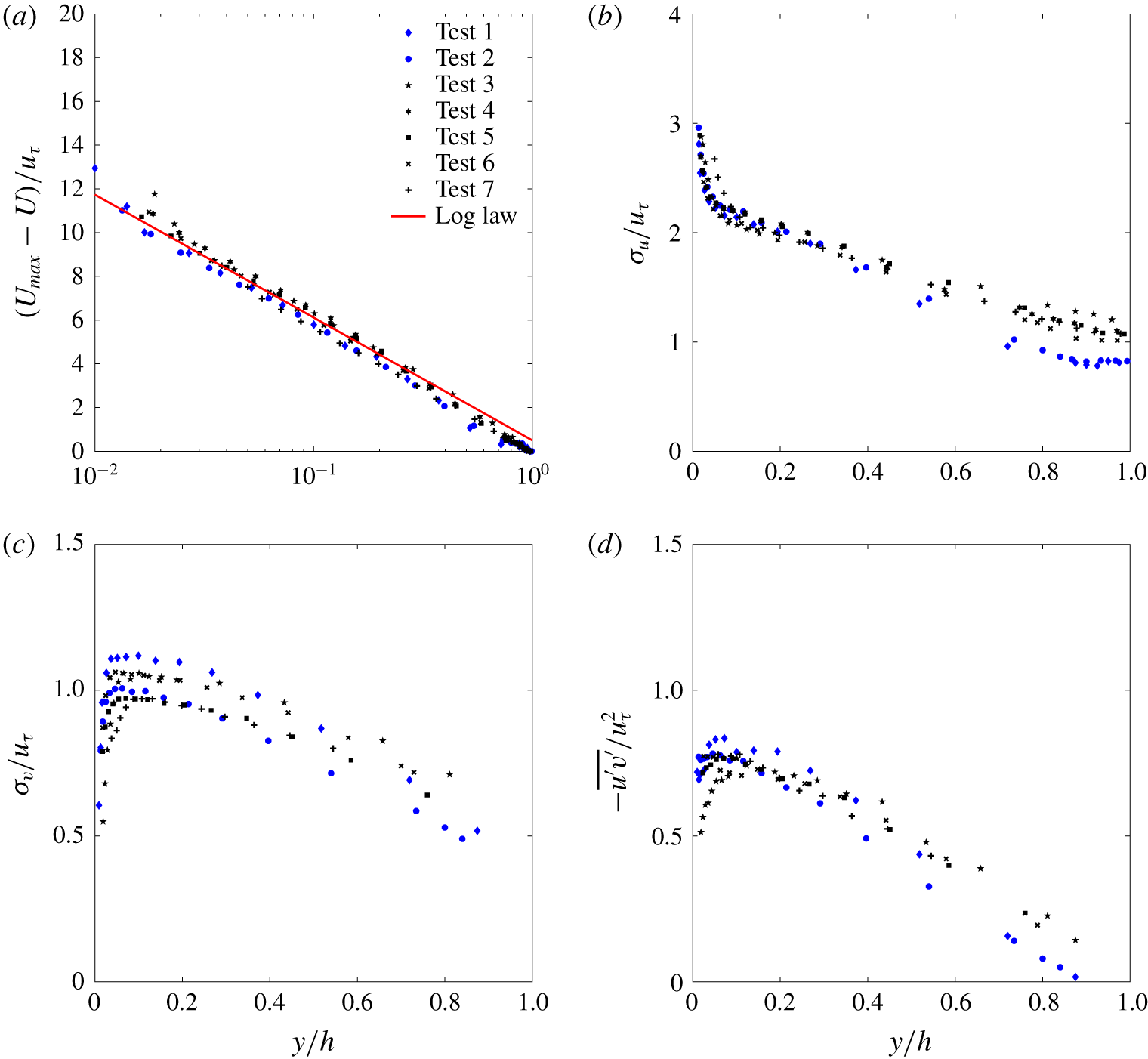
Figure 5. Outer scaling: (a) normalised streamwise mean velocity; (b) normalised standard deviation of the streamwise velocity fluctuations; (c) normalised standard deviation of the wall-normal velocity fluctuations; and (d) normalised Reynolds shear stress. The continuous line is the velocity-defect law.
3 Results
3.1 One-point statistics
Before addressing the issue of large-scale structures, an introductory section discussing classical one-point statistics is herein presented to validate the experimental methodology described in the previous section. This will be achieved by providing evidence that such statistics, when appropriately scaled, conform to data presented in the past literature. Furthermore, we believe that the following results might enrich the rather scarce set of published data on turbulence in smooth-bed open-channel flows and perhaps provide a benchmark for comparison with other canonical wall flows.
Figure 4 reports the first- and second-order velocity moments in classical inner scaling. Figure 4(a) reports the normalised longitudinal mean velocity profile together with the logarithmic law (2.3). It can be seen that, although the Clauser method to estimate  $u_{\unicode[STIX]{x1D70F}}$ was applied to a fixed range of elevations contained between
  $y^{+}=50$ and
  $y/h=0.2$ (as often done in wall turbulence studies), the upper boundary of the log region extends further away from the bed, i.e. up to
  $y/h=0.35$ (this is best seen in figure 5a).
Figures 4(b) and 4(c) report the non-dimensional standard deviation of the longitudinal ( $\unicode[STIX]{x1D70E}_{u}/u_{\unicode[STIX]{x1D70F}}$) and bed-normal (
 $\unicode[STIX]{x1D70E}_{v}/u_{\unicode[STIX]{x1D70F}}$) velocity components, respectively. Starting from
  $y^{+}>35$, figure 4(b) shows a systematic dependence of
  $\unicode[STIX]{x1D70E}_{u}/u_{\unicode[STIX]{x1D70F}}$ on
  $Re_{\unicode[STIX]{x1D70F}}$, as already extensively observed both in open-channel flows (Nezu & Nakagawa Reference Nezu and Nakagawa1993; Poggi et al. Reference Poggi, Porporato and Ridolfi2002) and in other wall flows (Durst, Jovanovi & Sender Reference Durst, Jovanovi and Sender1995; De Graaff & Eaton Reference De Graaff and Eaton2000; Marusic et al. Reference Marusic, McKeon, Monkewitz, Nagib, Smits and Sreenivasan2010; Smits, McKeon & Marusic Reference Smits, McKeon and Marusic2011).
The  $\unicode[STIX]{x1D70E}_{v}/u_{\unicode[STIX]{x1D70F}}$ profiles shown in figure 4(c) exhibit a plateau that increases its extent with increasing
  $Re_{\unicode[STIX]{x1D70F}}$. The
  $\unicode[STIX]{x1D70E}_{v}/u_{\unicode[STIX]{x1D70F}}$ value at the plateau is approximately 1–1.11, consistently with previous works on smooth-bed open-channel flows (Nezu & Nakagawa Reference Nezu and Nakagawa1993; Poggi et al. Reference Poggi, Porporato and Ridolfi2002) as well as other wall flows (Wei & Willmarth Reference Wei and Willmarth1989; Durst et al. Reference Durst, Jovanovi and Sender1995).
The normalised Reynolds shear stress profiles  $-\overline{u^{\prime }v^{\prime }}/u_{\unicode[STIX]{x1D70F}}^{2}$ follow a similar trend (figure 4d), showing a plateau that increases in extent (along the vertical coordinate) with increasing
  $Re_{\unicode[STIX]{x1D70F}}$. The value of
  $-\overline{u^{\prime }v^{\prime }}/u_{\unicode[STIX]{x1D70F}}^{2}$ at the plateau also increases with increasing
  $Re_{\unicode[STIX]{x1D70F}}$ from 0.75 to 0.85, reflecting the weakening of the viscous shear stresses with increasing Reynolds number. This behaviour is also in good agreement with past literature on open-channel flow studies (Nezu & Nakagawa Reference Nezu and Nakagawa1993; Poggi et al. Reference Poggi, Porporato and Ridolfi2002; Roussinova et al. Reference Roussinova, Biswas and Balachandar2008).

Figure 6. Measured (a) streamwise skewness, (b) wall-normal skewness, (c) streamwise kurtosis and (d) wall-normal kurtosis.
Figure 5 reports the first- and second-order velocity moments in classical outer scaling. For  $y/h>0.03$, mean velocity defects
  $U_{max}-U$ collapse very well (figure 5a) onto a curve described by the well-known logarithmic law in outer-scale normalisation:
 $$\begin{eqnarray}\frac{U_{max}-U}{u_{\unicode[STIX]{x1D70F}}}=-\frac{1}{\unicode[STIX]{x1D705}}\ln \left(\frac{y}{h}\right)+B_{1},\end{eqnarray}$$
 where  $B_{1}=0.5$ provides the best fit of the experimental data located at
  $y/h>0.03$. In general,
  $B_{1}$ is related to the wake strength parameter
  $\unicode[STIX]{x1D6F1}$ as
  $B_{1}=2\unicode[STIX]{x1D6F1}/\unicode[STIX]{x1D705}$. Kironoto & Graf (Reference Kironoto and Graf1995) report that the wake strength parameter retains a dependence on the non-uniformity parameter
  $\unicode[STIX]{x1D6FD}$ as
  $\unicode[STIX]{x1D6F1}=0.08\unicode[STIX]{x1D6FD}+0.23$. By using
  $\unicode[STIX]{x1D6FD}=-1.59$, which is the average taken over all the measured values of
  $\unicode[STIX]{x1D6FD}$ reported in figure 2,
  $\unicode[STIX]{x1D6F1}$ is equal to 0.103, which compares very well with
  $\unicode[STIX]{x1D6F1}={\textstyle \frac{1}{2}}\unicode[STIX]{x1D705}B_{1}=0.102$ if
  $\unicode[STIX]{x1D705}=0.41$.
Normalised standard deviations and shear Reynolds stresses (figure 5b–d) collapse fairly well, although, with respect to mean velocities, they display a slightly higher level of scatter. However, it should be noted that most of the scatter occurs for  $y/h>0.5$ and is due to the data pertaining to tests 1 and 2. This was reasonably expected because these experiments are characterised by a low aspect ratio, which makes velocity statistics susceptible to significant lateral-wall effects. Such effects are obviously expected to increase in significance with increasing distance from the bed. Focusing on the other high-aspect-ratio experiments, the scatter is within 10 %. As already discussed, this could be due either to different values of the
  $\unicode[STIX]{x1D6FD}$ parameter among the tests or to inaccuracy in the estimation of
  $u_{\unicode[STIX]{x1D70F}}$.
Figure 6 presents third- and fourth-order standardised velocity moments (skewness and kurtosis) in usual outer-scale coordinates. Except for tests 1 and 2, which display a different behaviour, all the experimental data for  $y/h>0.2$ collapse onto curves that resemble those published in the literature pertaining to open-channel flows over smooth walls (Poggi et al. Reference Poggi, Porporato and Ridolfi2002). With respect to the other tests, for
  $y/h>0.4$, tests 1 and 2 are characterised by significantly higher absolute values of skewness and kurtosis of both velocity components. The sign of
  $S_{u}$ and
  $S_{v}$ (figure 6a,b) suggests that ejection events in the outer layer are relatively more energetic in tests 1 and 2 than in the other tests. Furthermore, the higher values of
  $K_{u}$ and
  $K_{v}$ indicate that such events occur rather intermittently (i.e. more intermittently than in the other tests). The authors do not have an argument to explain why low aspect ratios should trigger such a different behaviour in terms of skewness and kurtosis, so these results are left as the subject of future investigations.
It is interesting to note that, for all tests, the skewness of the vertical velocity component  $S_{v}$ displays a peculiar behaviour whereby a plateau of
  $S_{v}\approx 0.17$ occurs over a range of distances from the bed which increases in extent with increasing
  $Re_{\unicode[STIX]{x1D70F}}$ but is always bounded below
  $y/h=0.2{-}0.3$ (figure 6b). As conjectured by Manes et al. (Reference Manes, Poggi and Ridolfi2011), the extent of the plateau and the way it depends on
  $Re_{\unicode[STIX]{x1D70F}}$ share a lot in common with the overlap (logarithmic) layer of the mean velocities. This can be somewhat justified by the fact that
  $S_{v}$ relates to part of the vertical turbulent flux of turbulent kinetic energy (i.e. the vertical turbulent transport of
  $\unicode[STIX]{x1D70E}_{v}^{2}$), which is expected to be constant in the overlap layer, where production and dissipation are in equilibrium (Townsend Reference Townsend1961; López & García Reference López and García1999).
3.2 Spectral analysis

Figure 7. Contour maps of the outer-scaled pre-multiplied 1-D spectra of the longitudinal velocity component  $(E_{xx}k_{x}/u_{\unicode[STIX]{x1D70F}}^{2})$ as a function of non-dimensional streamwise wavelength
  $(\unicode[STIX]{x1D706}_{x}/h)$ and distance from the wall
  $(y/h)$. The dashed lines indicate the bed-normal elevations where measurements were taken.
The 1-D power spectral density of the longitudinal velocity component  $E_{xx}(k_{x})$ in the wavenumber domain can be estimated from its frequency counterpart
  $E(f)$ by using the Taylor frozen-turbulence hypothesis (Taylor Reference Taylor1938). In particular, defining the streamwise wavenumber
  $k_{x}$ as
 $$\begin{eqnarray}k_{x}=\frac{2\unicode[STIX]{x03C0}f}{U_{c}},\end{eqnarray}$$
 where  $f$ is the frequency and
  $U_{c}$ is the eddy-convection velocity, the two power spectral densities are related by the following relation:
 $$\begin{eqnarray}E_{xx}(k_{x})=\frac{U_{c}}{2\unicode[STIX]{x03C0}}E(f).\end{eqnarray}$$
 In what follows,  $U_{c}$ was taken as the local mean velocity
  $U(y)$ at each elevation
  $y$ of interest.
It is well known that 1-D spectra suffer from aliasing effects (Tennekes & Lumley Reference Tennekes and Lumley1972), which artificially amplify the power spectral density of low-frequency components. Further significant distortions may arise from the use of the Taylor hypothesis, when passing from the frequency to the wavenumber domain, especially when studying turbulence in the near-wall region (Kim & Adrian Reference Kim and Adrian1999; Guala et al. Reference Guala, Hommema and Adrian2006; Del Álamo & Jiménez Reference Del Álamo and Jiménez2009; Cameron et al. Reference Cameron, Nikora and Stewart2017).
Despite these shortcomings, 1-D spectra have represented the key method to infer the scaling of large-scale structures in wall flows and hence, to allow for a direct comparison with past studies, they are also employed in the present paper. In order to minimise the spectral distortion due to the adoption of Taylor’s hypothesis, though, in what follows, results are discussed for the flow region above  $y/h=0.1$, where such distortion is significantly weaker than in the near-wall region (Nikora & Goring Reference Nikora and Goring2000). Results for
  $y/h<0.1$ are reported for completeness but are not discussed in depth and should be taken with care.
In order to provide a comprehensive picture of the energy distribution among different length scales, contour maps of pre-multiplied spectra are displayed in figure 7 for all the tests. The horizontal and vertical axes of each panel in figure 7 report the distance from the wall in outer scaling  $y/h$ and the normalised wavelength
  $\unicode[STIX]{x1D706}_{x}/h$, respectively (where
  $\unicode[STIX]{x1D706}_{x}=2\unicode[STIX]{x03C0}/k_{x}$). Figure 7 demonstrates the existence of a double peak in the pre-multiplied spectra at wavelengths commensurate with those reported in the literature on wall-bounded flows for LSMs (
 $\unicode[STIX]{x1D706}_{x}/h\approx \mathit{O}(1)$) and VLSMs (
 $\unicode[STIX]{x1D706}_{x}/h\approx \mathit{O}(10)$).
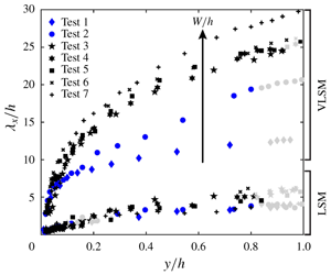
For high-aspect-ratio experiments (i.e. tests 3, 4, 5, 6 and 7 with  $W/h>5$), the spectral footprint of both LSMs and VLSMs lasts up to and, in some cases, even beyond
  $y/h=0.8$. This is at odds with what is observed in turbulent boundary layers and duct (i.e. closed-channel and pipe) flows (Monty et al. Reference Monty, Hutchins, Ng, Marusic and Chong2009), where VLSMs disappear at much lower
  $y/h$. Indeed, in turbulent boundary layers and duct flows only LSMs persist beyond
  $y/\unicode[STIX]{x1D6FF}\approx 0.2$ (Adrian et al. Reference Adrian, Meinhart and Tomkins2000; Balakumar & Adrian Reference Balakumar and Adrian2007; Monty et al. Reference Monty, Hutchins, Ng, Marusic and Chong2009) and
  $y/\unicode[STIX]{x1D6FF}\approx 0.6$ (Guala et al. Reference Guala, Hommema and Adrian2006; Monty et al. Reference Monty, Hutchins, Ng, Marusic and Chong2009), respectively. The persistence of the double peak in open-channel flows was also reported by Cameron et al. (Reference Cameron, Nikora and Stewart2017) and hence it seems to be a peculiarity of this class of flows.
The double peak is evident also for test 7 (figure 7g), which is characterised by a fairly low  $Re_{\unicode[STIX]{x1D70F}}=725$. This result supports the findings of Wang & Richter (Reference Wang and Richter2019), who report bimodal pre-multiplied spectra of the streamwise velocity component for
  $Re_{\unicode[STIX]{x1D70F}}$ as low as 550. Once again, this seems to be a peculiar characteristic of open-channel flows as, in canonical wall flows, Hutchins & Marusic (Reference Hutchins and Marusic2007b) identified a minimum
  $Re_{\unicode[STIX]{x1D70F}}\approx 1700$ for the VLSM peak to clearly appear in pre-multiplied spectra.
Low-aspect-ratio experiments (i.e. tests 1 and 2 with  $W/h<5$) display some differences with respect to the other tests. In particular, the peak pertaining to VLSMs disappears at
  $y/h=0.7$ and does not reach the water surface (figure 7a,b), as instead happens for tests 3–7 (figure 7c–g). Most importantly,
  $\unicode[STIX]{x1D706}_{x}/h$ for tests 1 and 2 are significantly smaller than in all other tests.

Figure 8. LSM and VLSM  $h$-normalised wavelength peaks in the pre-multiplied 1-D spectra of the longitudinal velocity component. The light grey markers indicate situations where LSM or VLSM peaks were not clearly detectable because poorly pronounced. The red line corresponds to the relation between normalised VLSM wavelengths and normalised elevations proposed by Monty et al. (Reference Monty, Hutchins, Ng, Marusic and Chong2009) for duct flows.
In order to have a clearer and general picture about the size and scaling of large-scale structures, figure 8 reports the wavelengths corresponding to spectral peaks pertaining to both LSMs and VLSMs for all experimental tests. Figure 8 also reports, for comparison, the empirical fit for VLSM wavelengths proposed by Monty et al. (Reference Monty, Hutchins, Ng, Marusic and Chong2009) for pipe and closed-channel flows, i.e.  $\unicode[STIX]{x1D706}_{x}/\unicode[STIX]{x1D6FF}=23(y/\unicode[STIX]{x1D6FF})^{3/7}$ (where
  $\unicode[STIX]{x1D6FF}=h$ for open-channel flows).
There are a lot of interesting features that emerge from figure 8. We begin by pointing out that LSM wavelengths scale well with the flow depth  $h$ regardless of flow conditions and resemble quite closely the results presented by Cameron et al. (Reference Cameron, Nikora and Stewart2017). VLSM wavelengths, instead, do not scale with the flow depth
  $h$ and are strongly dependent on the aspect ratio
  $W/h$. In fact, tests 3–6, which were carried out with a similar aspect ratio (i.e. spanning between approximately 5 and 7), are characterised by non-dimensional VLSM wavelengths
  $\unicode[STIX]{x1D706}_{x}/h$ collapsing well onto one curve. Test 7, instead, shows results deviating significantly from such a curve (especially for
  $y/h>0.35$), and it was carried out at a much higher aspect ratio (
 $W/h\approx 12$).
Perhaps the most interesting and striking result from figure 8 emerges from the data pertaining to the low-aspect-ratio experiments, namely tests 1 and 2. The non-dimensional VLSM wavelengths pertaining to these tests decrease quite dramatically over a rather small variation of  $W/h$ between 4.07 (test 2) and 3.05 (test 1). Such wavelengths also drop well below the curve identified by Monty et al. (Reference Monty, Hutchins, Ng, Marusic and Chong2009) for channel and pipe flows. On the contrary, LSM wavelengths keep scaling well with the flow depth
  $h$ as for the other shallower flows.
One may argue that the effects of the aspect ratio  $W/h$ are not isolated in all these tests, as
  $Re_{\unicode[STIX]{x1D70F}}$ and
  $x/h$ also vary extensively. A careful examination of the data, though, indicates that this is unlikely. For example, comparison between tests 4 and 5 allows one to single out the effects of
  $x/h$ (which varies extensively between 145 and 297) on VLSM scaling as
  $W/h$ and
  $Re_{\unicode[STIX]{x1D70F}}$ are kept reasonably constant. Figure 8 indicates that such effects are indeed negligible. As far as
  $Re_{\unicode[STIX]{x1D70F}}$ is concerned, its effects are singled out reasonably well in tests 3–6, where it varies between
  ${\approx}1000$ and
  ${\approx}1900$. Again, the results from figure 8 indicate that non-dimensional VLSM wavelengths for all the other tests seem to be
  $Re_{\unicode[STIX]{x1D70F}}$-independent. Therefore, the only parameter that explains well the variations of VLSM wavelengths observed across all the tests is the aspect ratio
  $W/h$. This result provides further evidence to support the conjecture made by Cameron et al. (Reference Cameron, Nikora and Stewart2017) that VLSMs and LSMs scale with different parameters. In particular, our data demonstrate unambiguously that, while LSMs scale well with the flow depth, the size of VLSMs is dictated by the aspect ratio
  $W/h$. To further corroborate this result, 1-D spectra were also computed using the bulk velocity
  $U_{b}$ (table 1) instead of the local velocity
  $U(y)$ in (3.2) and (3.3), and the final conclusions (not shown here) proved to be independent of the choice of the convection velocity.

Figure 9. (a) Spectral energy associated with LSM peaks normalised with  $u_{\unicode[STIX]{x1D70F}}^{2}$; and (b) spectral energy associated with VLSM peaks normalised with
  $u_{\unicode[STIX]{x1D70F}}^{2}$. The light grey markers have the same meaning as described in figure 8. The error bars indicate the confidence interval bounds (with a 95 % confidence level).

Figure 10. Pre-multiplied 1-D spectra of the longitudinal velocity fluctuations for tests 5–5d at eight different outer locations. Test 5 was measured in the centreline of the flume, while tests 5a, 5b, 5c and 5d were measured at  $z/W=$ 0.08, 0.16, 0.24 and 0.33, respectively. Panels (a)–(h) refer to spectra measured at different bed-normal elevations
  $y/h$. Note the different
  $y$-axes limits of panels (a), (g) and (h) with respect to the others.
For completeness, in figure 9(a,b) we also show the spectral energy associated with both LSM and VLSM peaks reported in figure 8. The 95 % confidence interval for each spectral energy estimation is also provided to identify statistically significant differences between data. Since all data points were characterised by very similar confidence intervals, these are reported only for one test to avoid overcrowding the figure. In figure 9(a,b) the shear velocity squared provides a fairly good collapse of data, at least for  $y/h>0.4$. Below this level, namely for
  $0.1<y/h<0.4$, the energy pertaining to LSM peaks collapses very well for all tests (figure 9a). Instead, data points related to VLSM peaks seem to display some sort of stratification (figure 9b). It is difficult to discern whether this is dictated by
  $Re_{\unicode[STIX]{x1D70F}}$ or the aspect ratio
  $W/h$. However, since tests 2 and 5 were carried out at very similar
  $Re_{\unicode[STIX]{x1D70F}}$ (but very different
  $W/h$) and are characterised by the same energy in the VLSM peaks, it can be reasonably argued that
  $Re_{\unicode[STIX]{x1D70F}}$ effects are more likely to dictate the stratification of data. This is also in line with results pertaining to canonical smooth-wall flows where the
  $Re_{\unicode[STIX]{x1D70F}}$ dependence of the VLSM peak energy has already been extensively reported (Marusic et al. Reference Marusic, McKeon, Monkewitz, Nagib, Smits and Sreenivasan2010; Smits et al. Reference Smits, McKeon and Marusic2011).
Given the significant dependence of VLSM wavelengths on the aspect ratio  $W/h$ (see figure 8), it is natural to associate VLSMs with cellular secondary currents, normally observed in open-channel flows. These secondary flows are, indeed, known to be dictated in number, size and intensity by the aspect ratio
  $W/h$ and whose topological resemblance to VLSMs has already been suggested by various authors, so much so that one could speculate that secondary currents are the footprint of VLSMs on the mean flow (Adrian & Marusic Reference Adrian and Marusic2012). Secondary currents can be described as cells of longitudinal vorticity whose height and width are approximately equal to the flow depth and whose intensity decreases with increasing distance from the lateral walls. In close proximity of such walls, secondary cells are somewhat split and their structure altered significantly due to the presence of corners (Tominaga et al. Reference Tominaga, Nezu, Ezaki and Nakagawa1989; Nezu & Nakagawa Reference Nezu and Nakagawa1993; Wang & Cheng Reference Wang and Cheng2005; Rodríguez & García Reference Rodríguez and García2008).
On these premises, it becomes interesting to investigate the dependence of VLSM wavelengths (or wavenumbers) on the spanwise coordinate, because it represents a way of testing the response of VLSMs to variations in the structure and intensity of secondary currents, somewhat analogously to exploring the dependence of VLSMs on the aspect ratio  $W/h$. This is precisely what was investigated in experiments 5a–5d (table 1), whose results are reported in figure 10(a–h), where each panel reports pre-multiplied spectra measured at a specific elevation from the bed and various locations along the spanwise coordinate. Figure 10 indicates that, for
  $y/h\geqslant 0.25$, the VLSM peak reduces in intensity and increases in wavenumber (i.e. reducing in wavelength) while approaching the lateral wall, so much so that in the proximity of the free surface (i.e.
  $y/h=0.98$, figure 10h) the VLSM peak occurs only in the central cross-section of the flow and disappears any closer to the lateral wall. This suggests that lateral walls and, presumably, associated effects on the structure and intensity of secondary currents, alter VLSMs. Furthermore, these observations point towards the idea that the observed
  $W/h$ effects on VLSMs might be mediated by variations that
  $W/h$ imposes on the intensity and size of secondary currents.
Note that, as per VLSMs, the LSM peak also decreases in intensity while approaching the lateral wall but is not altered in wavenumber (see, in particular, figure 10c, d, e and f) until  $y/h\geqslant 0.9$ (see figure 10g and h) where, however, spectra display peaks that are probably the signature of coherent structures developing within the sidewall boundary layer.
4 Conclusions
A dataset of velocity measurements was collected in non-uniform smooth-bed open-channel flows over a wide range of hydraulic conditions. In order to validate the experimental methodology and assess the quality of the experimental data, classical one-point statistics obtained from measurements taken mostly in the mid-cross-section of the flume were first computed and discussed against literature data pertaining to open-channel flows and other canonical wall flows. The results revealed that, provided the aspect ratio of the flow is greater than 5, the velocity profiles resemble those reported in the literature on open-channel flows and other canonical flows. In contrast, flows with aspect ratio lower than 5 display velocity statistics profiles that are significantly affected by the lateral walls. As one would expect, such effects were observed to increase with increasing distance from the bed and prevented data from collapsing with those pertaining to high-aspect-ratio experiments. This was particularly evident for third- and fourth-order velocity statistics.
The key results of the present work were obtained from spectral analysis of velocity time series. Pre-multiplied 1-D spectra of the longitudinal velocity component revealed a double-peak behaviour at wavenumbers consistent with those associated with LSMs and VLSMs, as observed in past studies on open-channel and canonical wall flows. With respect to canonical wall flows, three key differences were observed: (i) the double-peak behaviour persists throughout most of the vertical extension of the flow domain, namely up to at least  $y/h=0.8$, while in canonical wall flows it disappears beyond
  $y/\unicode[STIX]{x1D6FF}=0.6$ at most; (ii) the VLSM peak appears in pre-multiplied spectra for
  $Re_{\unicode[STIX]{x1D70F}}$ as low as 725, whereas in canonical wall flows much higher values are known to be required (Hutchins & Marusic Reference Hutchins and Marusic2007b); and (iii) as argued by a recent study pertaining to uniform rough-bed open-channel flows (Cameron et al. Reference Cameron, Nikora and Stewart2017), we confirm that the scaling of VLSM wavelengths is controlled by the aspect ratio
  $W/h$, as
  $Re_{\unicode[STIX]{x1D70F}}$ and
  $x/h$ effects were observed to be negligible. In particular, non-dimensional VLSM wavelengths increase with increasing
  $W/h$. We also confirm that LSM wavelengths scale well with the outer length scale of the flow, namely
  $h$.
$h$.
For one hydraulic condition, vertical profiles of velocity time series were measured not only in the mid-cross-section of the flume but also at various positions along the spanwise coordinate  $z/W$. Results from spectral analysis indicated that the wavelength and magnitude of the VLSM peaks were much more dependent on the spanwise coordinate, than wavelengths pertaining to LSM peaks. It was argued that, since in open-channel flows the shape and intensity of secondary currents also vary across the spanwise extent of the channel, the dynamics of VLSMs and secondary currents might be closely linked, as argued by Adrian & Marusic (Reference Adrian and Marusic2012).
Acknowledgements
C.M. acknowledges the support of Compagnia di San Paolo through the grant scheme ‘Attrarre docenti di qualità dall’estero’. C.P. is grateful to Teodoro Lamonaca for technical assistance in the realisation of the experimental set-up. The associate editor and the three anonymous referees are gratefully acknowledged for their valuable comments.
Declaration of interests
The authors report no conflict of interest.


