


INTRODUCTION
Glacier mass balance, and therefore glacier extent, directly responds to atmospheric conditions. Land terminating mountain glaciers are largely controlled by summer temperature, which effects ablation in the summer season (Oerlemans, Reference Oerlemans2005). On the subantarctic islands, atmospheric drying likely is an additional driver for glacier retreat, which is presently observed (Gordon et al., Reference Gordon, Haynes and Hubbard2008; Favier et al., Reference Favier, Verfaillie, Berthier, Menegoz, Jomelli, Kay and Ducret2016). In this respect, the temporal and spatial pattern of glacier fluctuations can provide a sensitive measure of the climatic history. In the subantarctic region between 40°S and 60°S, the position and strengths of the Southern Hemisphere westerly winds control the distribution of precipitation (e.g., Lamy et al., Reference Lamy, Kilian, Arz, Francois, Kaiser, Prange and Steinke2010) and influence ocean circulation by supporting wind-driven upwelling of deep water in the Southern Ocean south of the polar front (PF) (e.g., Toggweiler, Reference Toggweiler2009; Fig. 1). The island of South Georgia (54–55°S, 36–38°W; Figs. 1 and 2A) is one of the few sites in the Southern Hemisphere mid-lower latitudes that provide terrestrial and coastal marine records of former glacier extent. This makes South Georgia a prime study site to better understand the drivers of Holocene climate changes in the subantarctic region.

Figure 1 (colour online) Map of the southwestern Atlantic Ocean showing the locations of South Georgia and the bordering land masses of South America, the Antarctic Peninsula (James Ross Island [JRI] and South Shetland Islands [SSI]), and East Antarctica. Positions of the southern Antarctic Circumpolar Current front (SACCF), the polar front (PF), the subantarctic front (SAF), and the subtropical front (STF) after Orsi et al. (Reference Orsi, Witworth and Nowlin1995).

Figure 2 (A) Overview map of the central part of South Georgia showing the modern perennial snow and ice cover and geographic terms mentioned in the text. (B) Digital elevation model of the surroundings of Little Jason Lagoon (LJL) at the northern shore of Cumberland West Bay (for location, see orange rectangle in panel A), with the coring location Co1305. Coloured lines indicate limits of glacier advances (stages 3 to 5) according to White et al. (Reference White, Bennike, Melles and Berg2017) and the locations of streams entering LJL today. (For interpretation of the references to colour in this figure legend, the reader is referred to the web version of this article.)
Correlation of glacier deposits from different sites on South Georgia is mainly based on relative weathering and soil development studies (Clapperton et al., Reference Clapperton, Sugden, Birnie and Wilson1989; Bentley et al., Reference Bentley, Evans, Fogwill, Hansom, Sugden and Kubik2007; White et al., Reference White, Bennike, Melles and Berg2017). Continuous records from lakes and marine inlets can complement the geomorphological evidence by providing high-resolution chronological constraints on both glaciation history and climate fluctuations. Here we present a sediment record of Holocene environmental changes from a marine inlet at the northern shore of South Georgia. We use a combination of elemental, biomarker, diatom, and stable isotope data to infer changes in glacier extent and environmental conditions in the terrestrial and marine catchments of the inlet. The results provide information on the timing of the deglaciation and Holocene glacier advances and retreats, thereby improving the picture of the temporal development of land-based glaciers on South Georgia. We compare our reconstructions with records from the Antarctic Peninsula Region and from southern South America.
STUDY AREA
South Georgia has a maritime climate with a mean annual temperature of +1.9°C (Grytviken weather station; Trouet and Van Oldenborgh, Reference Trouet and Van Oldenborgh2013). At present, the central mountain range is covered by extensive ice fields, feeding numerous outlet glaciers, some of which presently terminate at sea level as tidewater glaciers. Small local glaciers with source areas lower than 600 metres above sea level (m asl) exist in cirques and on plateaus at lower altitudes (Clapperton, Reference Clapperton1990).
Geomorphological features on land and adjacent marine and fjord landforms indicate that the island was extensively glaciated in the past (Clapperton et al., Reference Clapperton, Sugden, Birnie and Wilson1989; Bentley et al., Reference Bentley, Evans, Fogwill, Hansom, Sugden and Kubik2007; Graham et al., Reference Graham, Fretwell, Larter, Hodgson, Wilson, Tate and Morris2008; Hodgson et al., Reference Hodgson, Graham, Giffiths, Roberts, Ó Cofaigh, Bentley and Evans2014a; Barlow et al., Reference Barlow, Bentley, Spada, Evans, Hansom, Brader, White, Zander and Berg2016; White et al., Reference White, Bennike, Melles and Berg2017). Exposure dating of glacial erratics suggests that the recession of a last glacial maximum ice cap exposed lower elevations around 16±1.5 ka (White et al., Reference White, Bennike, Melles and Berg2017). A lake record from the Stromness Bay area points to biogenic lake sedimentation starting around 18.6 ka (Rosqvist et al., Reference Rosqvist, Rietti-Shati and Shemesh1999; Fig. 2A). The initial ice retreat was followed by an ice readvance into the fjords during the Antarctic cold reversal (ACR; 14.7–13 ka; Pedro et al., Reference Pedro, Bostock, Bitz, He, Vandergoes, Steig and Chase2016; Graham et al., Reference Graham, Kuhn, Meisel, Hillenbrand, Hodgson, Ehrmann and Wacker2017). Deglaciation of low-altitude sites was well under way in the early Holocene, documented by the onsets of biogenic sedimentation in lakes and peat lands (Van der Putten and Verbruggen, Reference Van der Putten and Verbruggen2005; Hodgson et al., Reference Hodgson, Graham, Roberts, Bentley, Ó Cofaigh, Verleyen and Vyverman2014b). In the mid-Holocene (“neoglacial” period), widespread growth of glaciers on South Georgia occurred (e.g., Clapperton et al., Reference Clapperton, Sugden, Birnie and Wilson1989; Bentley et al., Reference Bentley, Evans, Fogwill, Hansom, Sugden and Kubik2007; White et al., Reference White, Bennike, Melles and Berg2017). Tidewater glaciers advanced into the fjords on the northwestern side of the island (Bentley et al., Reference Bentley, Evans, Fogwill, Hansom, Sugden and Kubik2007), and smaller land-terminating glaciers expanded down to lower altitudes (e.g., Clapperton et al., Reference Clapperton, Sugden, Birnie and Wilson1989; Clapperton, Reference Clapperton1990; White et al., Reference White, Bennike, Melles and Berg2017). In the late Holocene, South Georgia experienced another period of glacier advances (e.g., Rosqvist and Schuber, Reference Rosqvist and Schuber2003; Bentley et al., Reference Bentley, Evans, Fogwill, Hansom, Sugden and Kubik2007; Roberts et al., Reference Roberts, Hodgson, Shelley, Royles, Griffiths, Deen and Thorne2010, van der Bilt et al., Reference Van der Bilt, Bakke, Werner, Paasche, Rosqvist and Solheim Vatle2017). Glacier advances were less extensive than in the mid-Holocene and showed variability on centennial time scales (van der Bilt et al., Reference Van der Bilt, Bakke, Werner, Paasche, Rosqvist and Solheim Vatle2017).
Our coring site was located in a coastal inlet (Little Jason Lagoon) on the northwestern shore of Lewin Peninsula (Fig. 2A). At present, the inlet is connected with Cumberland West Bay over a 0.5- to 1.5-m-deep sill. This results in marine conditions in the inlet and likely leads to sediment supply from suspensions and ice-rafted debris (IRD) originating from glaciers calving into Cumberland West Bay to the southwest of Little Jason Lagoon (e.g., Neumayer Glacier; Fig. 2A and B). The maximum water depth in the inlet is approximately 24 m (Melles et al., Reference Melles, Bennicke, Leng, Ritter, Viehberg and White2013). Several small streams enter Little Jason Lagoon (Fig. 2B), with runoff being subject to seasonal changes with a peak during the snowmelt in austral summer. Areas below about 200 m asl are covered by vegetation, which is characterized by tussock grass (Parodiochloa flabellata), other grasses (Festuca contracta and Deschampsia antarctica), subshrubs (Acaena spp.), rushes (Juncus spp. and Rostkovia magellanica), and mosses (Greene, Reference Greene1964). The catchment of Little Jason Lagoon (highest elevation is Jason Peak, 570 m asl) is presently free of permanent ice or snowfields. Moraine ridges and debris deposits point to periods of expanded local mountain glaciers in the catchment of the inlet (Fig. 2B). Clapperton et al. (Reference Clapperton, Sugden, Birnie and Wilson1989) identified five stages of glacier advances on South Georgia. The oldest moraine ridges around Little Jason Lagoon document glaciers reaching down to modern sea level and correlate to “stage 3” sensu Clapperton et al. (Reference Clapperton, Sugden, Birnie and Wilson1989). The deposits have weathering characteristics that are broadly consistent with a late-glacial formation (White et al., Reference White, Bennike, Melles and Berg2017). Another ice advance is represented by a suite of glacial deposits, which are the remnants of cirque glaciers extending down to about 30 m asl (White et al., Reference White, Bennike, Melles and Berg2017; Fig. 2B) and correlate with a mid-Holocene advance (“stage 4”; Clapperton et al., Reference Clapperton, Sugden, Birnie and Wilson1989). The youngest late Holocene (“stage 5” deposits; Clapperton et al., Reference Clapperton, Sugden, Birnie and Wilson1989) glacier advance was restricted to small mountain glaciers, which formed in the upper catchment above 250 m asl (White et al., Reference White, Bennike, Melles and Berg2017; Fig. 2B).
MATERIALS AND METHODS
Coring
Sediment coring on Little Jason Lagoon was carried out in March 2013 within the scope of the expedition ANT XXIX/4 of R/V Polarstern (Melles et al., Reference Melles, Bennicke, Leng, Ritter, Viehberg and White2013). Coring was conducted in the deepest part of the lagoon from a platform. A gravity corer (UWITEC Ltd., Austria) was used for sampling of the uppermost sediment decimetres and the sediment–water interface. Deeper sediments were sampled using a percussion piston corer (UWITEC Ltd.). The piston cores retrieved from Little Jason Lagoon overlap by about 1 m. The final core composite of core Co1305 has a length of 11.04 m; it consists of seven gravity and piston cores, which were correlated on the basis of core descriptions and analytical data (X-ray fluorescence [XRF]–elemental scans and water content) in overlapping core segments.
Core processing and physical properties
The sediment cores were stored at 4°C until opening in the laboratory. One core half was used for nondestructive analysis—that is, line-scan imaging with a multisensor core logger (GeoTek, UK), XRF scanning (see next section), and core description. For analyses of discrete samples, the working half of the composite core was subsampled in 2 cm slices. The sediment samples were freeze-dried, and the water content was determined by weight loss during freeze-drying.
As a proxy for IRD, the number of particles >1 mm in diameter was quantified for 47 samples. For that purpose, 6 to 25 g of wet sediment (corresponding to subsampled 2 cm sediment slices) was wet sieved on a 1 mm steel mesh sieve. The number of mineral grains retained on the sieve was counted and normalized to the dry sediment weight of the respective samples.
Elemental analysis
The chemical composition of the sediment core was investigated at 2 mm resolution by XRF scanning, using an ITRAX XRF core scanner (Cox Ltd.; Croudace et al., Reference Croudace, Rindby and Rothwell2006). Measurements were performed with a chromium X-ray tube with 30 mA, 30 kV, and an exposure time of 20 s. Results are given as counts per second (cps), which is a semiquantitative measure of element concentration, or as element count ratios.
Furthermore, quantitative elemental analyses of total sulphur (S) and total carbon (C) were conducted on 86 aliquots of ground sediment samples with a Vario Micro Cube combustion elemental analyser (EA; Elementar, Germany), and total inorganic carbon (TIC) was quantified on parallel samples with a DIMATOC 200 (DIMATEC Corp.).
Stable isotope analysis
The δ13C values of the bulk organic matter (OM) and the corresponding C/N ratios can be indicative for the sources of OM—that is, they can be used to distinguish freshwater, terrestrial, and marine sources of OM and hence indicate depositional environments (e.g., Leng and Lewis, Reference Leng and Lewis2017). δ13C ratios and the C/N concentrations were determined on 75 samples with equal sampling intervals. In preparation of the measurements, freeze-dried sediment samples were treated with 5% HCl to remove any CaCO3 and then washed thrice in 500 mL deionised water. After drying at 40°C, the material was ground to a fine powder using an agate pestle and mortar. δ13C analyses were performed by combustion in a Costech ECS4010 EA online coupled to a VG TripleTrap (plus secondary cryogenic trap) and Optima dual-inlet mass spectrometer. We use the C and N values obtained with the EA during the isotope analysis for calculating the C/N ratio. Percent C analyses were calibrated against an Acetanilide standard. The δ13C values were calculated to the Vienna Pee Dee belemnite scale using a within-run laboratory standard (BROC2) calibrated against NBS-19 and NBS-22. Replicate analysis of well-mixed samples indicated a precision of <0.1‰ (1 standard deviation).
Diatom analysis
Diatom analysis was carried out on 12 samples with equal sampling intervals to determine the depositional environment and hence to distinguish lacustrine from marine conditions. Quantitative preparation of diatom slides was conducted on 0.01 to 0.025 g of dried sediment following the settling method of Scherer (Reference Scherer1994). Diatom counting was carried out on a light microscope at ×1000 magnification. Where possible, a minimum of 300 specimens were counted and identified to the species or genus level. Taxonomic classification follows that of Hasle and Syvertsen (Reference Hasle and Syvertsen1997), supplemented with descriptions of Antarctic species by Krebs (Reference Krebs1983), Johansen and Fryxell (Reference Johansen and Fryxell1985), and Scott and Thomas (Reference Scott and Thomas2005).
Diatom species were grouped into freshwater diatoms (e.g., Achnanthidium minutissimum, Amphora veneta, Craticula sp., Cymbella cistula, Discostella stelligera, Diploneis sp., Discostella stelligera, Fragilaria capucina, Fragilaria germainii, Fragilaria tenera, with D. stelligera and small Fragilariaceae, such as Staurosirella sp., Psuedostaurosira spp., etc., being the most dominant ones) and marine diatoms (e.g., Chaetoceros hyalocheate vegetative cells, Chaetoceros resting spores, Thalassiosira antarctica, Odontella litigiosa, and Fragilariopsis spp.). The remainder of the diatom species comprise marine benthic and brackish taxa, including Cocconeis spp. and Navicula spp., which have been merged, because there is considerable overlap between their habitats. A summary of diatom species identified in sample of core Co1305 is given in the Supplementary Table 1.
Lipid biomarker analysis
The concentration and distribution of n-alkanes with chain lengths of 25 to 35 carbon atoms (C25–C35) were analysed in 33 samples from 5-cm-thick layers sampled in 50 cm intervals from core Co1305. The high-molecular-weight n-alkanes are compounds of leaf waxes of higher land plants and thus can be used as terrestrial biomarkers in sediments (review by Pancost and Boot, Reference Pancost and Boot2004). The n-alkanes were extracted from the sediment samples by accelerated solvent extraction (ASE 300, Thermo, USA) using dichloromethane (DCM) and methanol (MeOH) (9:1, v/v at 120°C, 75 bar) yielding total extractable lipids (TLEs). The TLEs were saponified with 0.5 M KOH in MeOH and water (9:1, v/v) at 80°C for 2 h and desulfurized using activated copper. Neutral lipids were extracted from TLEs with DCM by liquid-liquid phase separation from which n-alkanes were purified by column chromatography (SiO2, deactivated, mesh 60) and elution with hexane. Individual compounds were identified and quantified by gas chromatograph (GC; Agilent 7890B, Agilent Technologies, USA) with a flame ionization detector (FID) and using an external standard (n-alkanes C21 to C40, 40 mg/L each; Sigma Aldrich). The GC was equipped with a 50 m DB5 MS column (0.2 mm internal diameter [i.d.] and 0.33µm film thickness by Agilent Technologies). Concentrations are normalized to the total organic carbon (TOC) content of the respective samples (µg/g TOC), which was analysed on aliquots of the original sediment samples with a DIMATOC 200 (DIMATEC Corp.).
In living plants, odd-numbered n-alkanes dominate over even-numbered homologues (Eglinton and Hamilton, Reference Eglinton and Hamilton1963). When plant material is degraded in soils or peat deposits (e.g., by microbial activity), the even-numbered homologues become more abundant. We calculated the carbon preference index (CPI) for odd over even dominance for C25–C35 (after Marzi et al., Reference Marzi, Torkelson and Olson1993) to use it as a source indicator as well as a measure of degradation of the organic material.
Radiocarbon dating and core chronology
For age assignment of the sediment sequence, we conducted radiocarbon (14C) analysis on different organic materials. Macroscopic plant fossils were mainly preserved in the lower part of the core and could be picked from six depths. In the upper part (105 cm depth), a kelp fragment and a mollusc shell were found, which were used for 14C analysis. A second carbonate fossil could be dated from 264 cm depth. If no macrofossil could be selected, bulk organic carbon (OC) was dated (eight samples throughout the core). For the determination of a present-day local marine reservoir age, we dated a recent carbonate shell of a marine mollusc, which was sampled on the beach of Grytviken. Because bulk OC contains a mixture of OM from various sources, 14C ages do not necessarily reflect the sedimentation age. In the setting of Little Jason Lagoon, OM is not only derived from autochthonous marine production, but also contains older, (glacially) reworked carbon as well as terrestrial OM from plant remains and soils. We thus additionally use compound-specific 14C analysis of lipid biomarkers to better constrain the source and time of delivery from land into the sediment of the dated material. As biomarkers derived from terrestrial vascular plants may be considerably older because of intermediate storage in soils (e.g., Drenzek et al., Reference Drenzek, Montucon, Yunker, Macdonald and Eglinton2007), we use the n-C16 fatty acids (FAs,) which are a common compound of aquatic and marine biomass (e.g., phytoplankton; Volkman et al., Reference Volkman, Johns, Gillan, Perry and Bavor1980). Previous studies in this region have shown that n-C16 FA ages reflect the value of dissolved inorganic carbon during OM formation (Ohkuchi and Eglinton, Reference Ohkuchi and Eglinton2008) and therefore have the potential to provide the sediment age (e.g., Uchida et al., Reference Uchida, Shibata, Kawamura, Kumamoto, Yoneda, Ohkushi and Harada2001).
Sample preparation for 14C analysis was done using standard methods (Rethemeyer et al. (Reference Rethemeyer, Dewald, Fülöp, Hajdas, Höfle, Patt, Stapper and Wacker2013). Briefly, bulk OC and macrofossil samples were decarbonised with acid and converted into CO2 by combustion. Carbonate samples were leached with acid and subsequently converted into CO2 with phosphoric acid. The CO2 was transformed into graphite cathodes using automated graphitization equipment (AGE, Ionplus, Switzerland). Accelerator mass spectrometry (AMS) measurements were carried out at the CologneAMS facility (University of Cologne, Germany; Dewald et al., Reference Dewald, Heinze, Jolie, Zilges, Dunai, Rethemeyer and Melles2013).
For compound-specific radiocarbon analyses, FAs were separated from TLEs after acidification with HCl by liquid-liquid phase separation and subsequent open column chromatography as described in Höfle et al. (Reference Höfle, Rethemeyer, Mueller and John2013). FAs were transferred to fatty acid methyl esters using MeOH with known 14C content to correct the results for the carbon added. The purification of the n-C16 FAs was conducted by preparative capillary gas chromatography. The system consists of a GC (7680 Agilent Technologies) equipped with a CIS 4 injection system (Gerstel, Germany) and is coupled with a preparative fractionation collector (PFC; Gerstel). Chromatographic separation was done with a “megabore” ultra–low bleed capillary column (30 m, 0.53 mm i.d.; Restek, USA), and trapping of n-C16 FAs with the PFC was achieved at room temperature. The purity and quantity of trapped compounds was analysed by GC-FID (on-column, Agilent 7890B, Agilent Technologies). The isolated n-C16 FAs were transferred into quartz tubes with copper oxide (CuO) and silver (Ag) added and vacuum sealed. Quartz tubes, CuO and Ag were precombusted (900°C, 4 h) prior to use. Samples were combusted at 900°C to form CO2. The CO2 was purified cryogenically and analysed on a MICADAS AMS system using its gas ion source (ETH Zurich, Switzerland; Wacker et al., Reference Wacker, Bonani, Friedrich, Hajadas, Kromer, Nemec, Ruff, Suter, Synal and Vockenhuber2010). Compound ages were corrected for process blank and methylation by mass balance calculation following the procedure described by Rethemeyer et al. (Reference Rethemeyer, Dewald, Fülöp, Hajdas, Höfle, Patt, Stapper and Wacker2013).
RESULTS
Lithology, sediment composition, and environmental settings
Based on the lithology; the elemental, biomarker, and diatom compositions; and the stable isotope data, the 11.04-m-long core composite Co1305 was divided into four distinct units (Fig. 3J). Because TIC values were not distinguishable from background in all analysed samples, we considered the C content to be similar to TOC concentration.

Figure 3 (colour online) Lithology and proxy data of the core composite Co1305 versus sediment depth. Major lithologic characteristics (A); radiocarbon ages (14C yr BP) (B); ice-rafted debris (IRD) given as grains >1 mm per gram dry sediment (C); Ti counts (cps) and Si/Ti ratio (10-point running average) (D); C25 to C35 n-alkanes (µg per gram TOC) and proportion of leaf wax–derived high-molecular-weight (HMW) n-alkanes C27,C29, C31 (%) (E); total carbon (C) and total sulphur (S) content (%) (F); water content (%) (G); C/N ratio and δ13C of organic carbon (H); proportions of fresh water (fresh), brackish/benthic (b/b), and marine diatom species (I); and lithologic units (J).
Unit I (1104–1042 cm)
Unit I consists of a grey diamicton, which contains a mixture of sand, silt, and clay, as well as interspersed rock fragments with diameters of up to several centimetres. A very low water content of about 14 wt% in the lower part (1104 to 1066 cm) suggests overconsolidation (Fig. 3G). The sediment becomes successively wetter and less coarse grained in the uppermost approximately 20 cm. These sediment characteristics point to deposition in a subglacial environment (basal till), possibly passing into a proglacial environment in the upper part (waterlain till; e.g., Eyles et al., Reference Eyles, Mullins and Hine1991).
A subglacial to proglacial deposition of unit I is supported by the elemental and biomarker data. The C and S contents throughout the unit with <0.3 wt% and <0.2 wt%, respectively, are minimal (Fig. 3F). A specific source of OM cannot clearly be assigned based on the δ13C values and C/N ratios (Fig. 4). δ13C values of –26.0±0.1‰ could originate from lacustrine or land-plant sources, whereas the low and variable C/N ratios (6.5±1.0) may reflect a bacterial origin (Lamb et al., Reference Lamb, Wilson and Leng2006; Leng and Lewis, Reference Leng and Lewis2017). From one sample (1048 cm depth), n-alkanes were extracted (24 µg/g TOC) (Fig. 3E), which were dominated by homologues of C29 and C31 carbon atoms and had a CPI of 5.7 characteristic for soil-derived, slightly humified OM (Andersson and Meyers, Reference Andersson and Meyers2012; Angst et al., Reference Angst, John, Mueller, Kögel-Knabner and Rethemeyer2016) (Fig. 5). The OM in unit I most likely originates from reworked allochthonous sources.

Figure 4 (colour online) δ13C of organic carbon versus C/N ratio of the organic matter (measured on the same aliquot). The lithologic units can be clearly distinguished by their δ13C and C/N signatures. Typical δ13C and C/N ranges for organic inputs are given (after Lamb et al., Reference Lamb, Wilson and Leng2006).
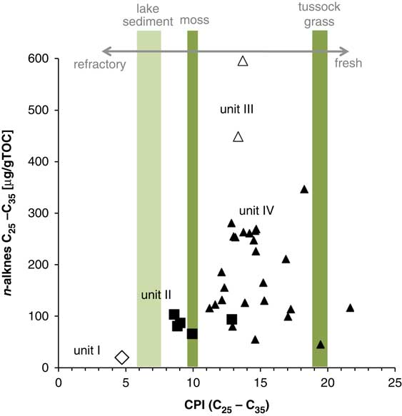
Figure 5 (colour online) n-Alkane concentrations (C25 to C35) of sediment samples from core Co1305 versus carbon preference index (CPI). CPI was calculated for chain lengths of C25 to C35 [CPI=((C25 + C27 + ... C33) + (C27 + C29 + ... C35)) / 2 × (C26 + C28 + ... C34); Marzi et al., Reference Marzi, Torkelson and Olson1993]. For reference, CPI values of tussock grass and a terrestrial mosses sampled from the catchment of Little Jason Lagoon are given, as well as the range of CPI values of lake sediments from Holocene sediments of a lake on Lewin Peninsula.
Unit II (1042–996 cm)
Unit II consists of finely laminated silt and clay with some irregularly interspersed rock fragments and mineral grains in the >1 mm fraction (Fig. 3C). These coarse-grained particles in a very fine-grained matrix most likely represent IRD (Grobe, Reference Grobe1987 and references therein), originating either from icebergs (as supraglacial, englacial, or subglacial debris) or from lake ice floats (because of basal freeze-on or surface spill close to the shore) as suggested for Arctic lake and marine environments (Smith, Reference Smith2000; Sakamoto et al., Reference Sakamoto, Ikehara, Aoki, Iijima, Kimura, Nakatsuka and Wakatsuchi2005). The fine-grained lamination furthermore points to a low energetic depositional environment. In the lower part of unit II, laminae are formed by alternating proportions of dispersed OM and siliciclastic components. Above 1026 cm, interspersed macroscopic moss fragments form discrete sediment layers. There, significant biogenic production and accumulation are also evidenced by C and S contents of about 1.2 wt% (Fig. 3F).
Diatom concentrations in unit II have a mean value of 7 million valves per gram sediment (Mv/g; Supplementary Table 1). The diatom Discostella stelligera dominates during this interval. It is a freshwater planktonic taxon, which is common in oligotrophic lakes in Greenland and elsewhere in the Arctic (e.g., Saros and Anderson, Reference Saros and Anderson2015). A freshwater origin of parts of the OM in unit II is also reflected by low δ13C values (–28.1±0.5‰) and C/N ratios of 8.5±0.3 (Fig. 4). Concentrations of leaf wax n-alkanes range from 73 to 115 µg/g TOC (95±16 µg/g TOC; Fig. 3E), and CPI values of about 9 (Fig. 5) reflect input of less decomposed soil OM than in unit I and larger contributions of higher terrestrial plants into the lake.
Unit III (996–978 cm)
Sediments in unit III are finely laminated and fine grained (silt and clay), suggesting that the low-energy environment of unit II persisted during the formation of unit III. The same holds true for the lack of bioturbation, possibly because of a reduced ventilation of the water column. One sample was checked for mineral grains in the >1 mm sieve fraction (from 986 cm depth) and did not contain any IRD (Fig. 3C).
The diatom assemblage in the one sample analysed from unit III (986 cm; Fig. 3I) contains 3% of counted diatoms from the freshwater group, whereas brackish/benthic and marine diatoms contribute almost equal amounts of 41% and 56%, respectively (Fig. 3I). This indicates a change to more saline conditions, likely because of a marine ingression. A transition from lacustrine to marine conditions is supported by a significant increase in δ13C values throughout unit III (Figs. 3H and 4), which is indicative for the incorporation of marine OM (Leng and Lewis, Reference Leng and Lewis2017). The transition is accompanied by an increase in S in the sediments of unit III, which reaches a maximum of 4 wt% at 994 cm depth.
The C content in unit III increases, ranging from 1.9 to 2.5 wt% (Fig. 3F). δ13C values point to autochthonous origin of OM (e.g., from diatoms and other phytoplankton groups; Figs. 3H and 4). However, larger contributions of terrestrial OM are indicated by slightly higher C/N ratios in unit III (9.0–10.9) compared with unit II (8.5±0.3; Figs. 3H and 4). The input of higher plant-derived OM is supported by a maximum concentration of C25–C35 n-alkanes in the two samples analysed from unit III (634 and 480 µg/g TOC; Fig. 3E) and by the high CPI values of 13, which are within the range of fresh plant material (Fig. 5).
Unit IV (978–0 cm)
Sediments of unit IV are layered at a centimetre scale. The material is generally fine grained (silt and clay) with changing minor proportions of sand and gravelly IRD (Fig. 3C). This is also reflected by centimetre-scale variations in Ti, which is exclusively of minerogenic origin and therefore indicates recurring changes in siliclastic input (Fig. 3D). Changes in the inorganic composition of the sediments in unit IV are suggested by changes in the Si/Ti ratio (Fig. 3D). In contrast to Ti, Si can also be derived from biogenic silica, produced by diatoms and sponges. Changes in the Si/Ti ratio may therefore reflect changes in the proportion of biogenic silica and siliclastic material. C concentrations in unit IV range from 0.9 to 3.3 wt% (mean 2.0±0.5 wt%) with lowest OC contents between 938 and 714 cm depth (Fig. 3F).
The dominance of marine diatoms (84–93%; Fig. 3I) throughout unit IV indicates full marine conditions. The frustules are well preserved, and Chaetoceros resting spores (82–93%) dominate the assemblage, suggesting high productivity within a seasonally stratified water column (Hargraves and French, Reference Hargraves and French1983). The benthic species in unit IV are frequently found in the Antarctic Peninsula region. They are cold-water taxa not specifically associated with sea ice (Lange et al., Reference Lange, Tenenbaum, De Santis Braga and Campos2007; Al-Handal and Wulff, Reference Al-Handal and Wulff2008a, Reference Al-Handal and Wulff2008b). Marine conditions are also indicated by high δ13C values (–20.3±0.6‰) and low C/N ratios (7.4±0.3), which are typical for OM derived from marine algae (Fig. 4). An additional indication comes from the occurrence of marine macroalgae (kelp), in particular above 502 cm (Fig. 3A).
Concentration of land-plant-derived n-alkanes, ranging from 46 to 347 µg/g TOC (with a mean of 143±67 µg/g TOC), and CPI values from 11 to 21 (Fig. 5) reflect high but variable inputs of land-plant-derived material into the inlet (Fig. 3E).
Core chronology
A total of 24 14C ages were obtained for core Co1305. Ages range from 660±40 14C yr BP (plant fossil in 10 cm depth) to 14,170±70 14C yr BP for bulk OC from the base of unit II (Figs. 3B and 6A, Table 1). Bulk OC ages become successively older with depth, except for one data point. However, 14C ages of bulk OC are significantly older than those of carbonates and plant remains from similar or lower core levels (Fig. 6A) suggesting that the sediments contain high and variable proportions of older C and do not reflect the actual age of sedimentation.

Figure 6 (colour online) Radiocarbon ages and age-depth model for core Co1305. (A) Conventional 14C ages (yr BP) from bulk organic matter (OM), n-C16 fatty acids (FAs), and terrestrial (moss) and marine (kelp and carbonate) fossils shown versus depth. 14C ages shown here are not corrected for reservoir age. (B) Age-depth model created by polynomial interpolation between neighbouring levels (Clam 2.2.; Blaaw, Reference Blaaw2010). The model is based on the n-C16 FA ages, carbonate, and marine macroalgae. Calibrated ages of plant remains provide maximum ages of deposition for unit II.
Table 1 Conventional 14C ages obtained for bulk organic matter (OM), n-C16 fatty acids (FAs), carbonates, and plant debris (kelp and mosses) from sediments of core Co1305. 14C value of 720 yr for a modern carbonate shell from Grytviken was used to estimate a marine reservoir correction. A constant value was used to correct samples of marine origin (carbonates, n-C16 FAs, and kelp) for a local reservoir effect (14C age corr.). Age ranges of calibrated ages are given for samples, which are considered in our interpretation. Marine samples were calibrated with the data set Marine13 (ΔR=320 yr; Reimer et al., Reference Reimer, Bard, Bayliss, Beck, Blackwell, Bronk Ramsey and Buck2013), and samples of terrestrial (terr.) origin were calibrated with SHCal13 (Hogg et al., Reference Hogg, Hua, Blackwell, Buck, Guilderson, Heaton and Niu2013). pmC = percent modern Carbon.

The 14C ages of n-C16 FAs are younger than those in bulk OC, and they are in good agreement with 14C ages of the kelp and carbonate macrofossils selected from 105 cm core depth suggesting a common marine source (Fig. 6A, Table 1). The uncalibrated 14C ages of two mosses dated from unit III are ca. 800 yr older than the n-C16 FAs from the corresponding core depth (Fig. 6A, Table 1). Much older plant fossils, which probably do not reflect sediment age, were also found in other lake sediment records from South Georgia (Strother et al., Reference Strother, Salzmann, Roberts, Hodgson, Woodward, Van Nieuvenhuyze, Verleyen, Vyverman and Moreton2015; van der Bilt et al., Reference Van der Bilt, Bakke, Werner, Paasche, Rosqvist and Solheim Vatle2017). The age offset likely results from long transport times or intermediate storage in the catchment prior to deposition in the sediment. In Little Jason Lagoon, the n-C16 FA age likely best reflects the sediment age by providing a 14C signal of aquatic production rather than of potentially preaged terrestrial OM.
Because of the scarcity of datable macrofossils in the sediments and the potentially reworked origin of terrestrial OM in Little Jason Lagoon, we also use n-C16 FA ages for the age-depth model of core Co1305. This, however, requires correction for the marine reservoir effect. Benthic foraminifers from the shelf off South Georgia provided 14C ages of 1100 yr and reflect the marine reservoir age (Graham et al., Reference Graham, Kuhn, Meisel, Hillenbrand, Hodgson, Ehrmann and Wacker2017). However, this value probably does not reflect the local reservoir age in Little Jason Lagoon. Carbonates in 105 and 264 cm core depth gave 14C ages of 1055±45 and 1180±40 yr BP, respectively. A reservoir correction of 1100 yr would imply unreasonably high sedimentation rates for the upper 260 cm of the sequence. The reservoir age in Little Jason Lagoon is likely lower than in the open marine setting and more likely reflected by the 720 yr obtained from the recent, shallow-water carbonate shell (Table 1). The modern carbonate shell can be affected by elevated 14C concentration because of its postbomb origin, which leads to an underestimation of the prebomb reservoir age. Gordon and Harkness (Reference Gordon and Harkness1992) suggested a prebomb reservoir correction of ca. 750 yr for South Georgia, which is in accordance with our findings. The difference in reservoir ages in the benthic foraminifers and the littoral carbonate could be because of the different carbon sources related to different water masses. Temperature and salinity profiles from Cumberland Bay indicate that the upper 25 m of the water column are influenced by local meltwater, whereas Antarctic Surface Water and Circumpolar Deep Water fill the deeper parts of the fjord (Geprägs et al., Reference Geprägs, Torres, Mau, Kasten, Römer and Bohrmann2016).
To account for the local reservoir effect, we use a constant reservoir correction of 720 yr for marine samples. It is highly likely that the reservoir age changed through time. Variable freshwater runoff, relative sea-level (RSL) change, or changes in ocean circulation throughout the record may have changed the reservoir age. The quantification of such changes is not possible based on the data available and leads to some uncertainty in the age determination of the sediments and the in the age-depth model. For the establishment of an age depth-model, terrestrial samples were calibrated with the SHCal13 data set (Hogg et al., Reference Hogg, Hua, Blackwell, Buck, Guilderson, Heaton and Niu2013) and samples of marine origin were calibrated with the Marine13 data set (Reimer et al., Reference Reimer, Bard, Bayliss, Beck, Blackwell, Bronk Ramsey and Buck2013) using a reservoir correction of 720 yr (ΔR=320 yr). The age-depth model of core Co1305 was developed with the software Clam 2.2 (Blaaw, Reference Blaaw2010) by a third-order polynomial regression (Fig 6B).
DISCUSSION
Late Pleistocene deglaciation (>11.2 ka)
The till recovered in Co1305 shows that the Little Jason Lagoon was glaciated. The occurrence of vascular plant n-alkanes in the lake sediments above the till points to the presence of catchment vegetation from the beginning of lake sedimentation. The soils surrounding Little Jason Lagoon therefore had stabilised by that time, which is also suggested by the diatom D. stelligera, which is typically not found in lakes immediately after local deglaciation and becomes abundant only once there is enough N and light available (Perren et al., Reference Perren, Axford and Kaufman2017).
The glacial sediments in Little Jason Lagoon could correspond to an ice cap that covered Lewin Peninsula and had retreated from lower elevations around 16±1.5 ka (“stage 1–2”; Clapperton et al., Reference Clapperton, Sugden, Birnie and Wilson1989, White et al., Reference White, Bennike, Melles and Berg2017). However, the lake record indicates that some terrestrial vegetation already became established with the onset of lake sedimentation. Thus, we interpret unit I as a till produced by a local glacier flowing out of the Little Jason Lagoon catchment towards Jason Harbour from Jason Peak, which is consistent with the “stage 3” (Clapperton et al., Reference Clapperton, Sugden, Birnie and Wilson1989) moraine ridges around Little Jason Lagoon that postdate an ice cap retreat and document an expansion of local mountain glaciers down to modern sea level (White et al., Reference White, Bennike, Melles and Berg2017). The plants may have survived a late-glacial advance (“stage 3”) in areas unaffected by glacier overriding and thus could disperse rapidly after glaciers retreated. This could explain the occurrence of terrestrial OM in the lake shortly after local glacier retreat. The RSL was several metres below the present prior to 12 ka (Barlow et al., Reference Barlow, Bentley, Spada, Evans, Hansom, Brader, White, Zander and Berg2016), and land areas were exposed that are now below sea level. On these grounds, land plants could have grown at the same time as glaciers terminated close to present sea level.
Based on the radiocarbon age of 14,870–15,370 cal yr BP of moss fragments, which were found in 1034 cm depth in unit II (COL2842; Table 1, Fig. 7E), this glacier advance can be tentatively correlated to the ACR time slice, when tidewater glaciers readvanced in Cumberland East Bay (15.2±0.3 to 13.3±0.15 ka; Graham et al., Reference Graham, Kuhn, Meisel, Hillenbrand, Hodgson, Ehrmann and Wacker2017; Fig. 7N), and perhaps also in Stromness Harbour (13.5±1.5 ka; Bentley et al. [Reference Bentley, Evans, Fogwill, Hansom, Sugden and Kubik2007] recalculated to Borchers et al. [Reference Borchers, Marrero, Balco, Caffee, Goehring, Lifton, Nishiizumi, Phillips, Schaefer and Stone2016] production rate; Fig. 7J). The ACR has been identified in marine and ice core records from Antarctica (Mulvaney et al., Reference Mulvaney, Abram, Hindmarsh, Arrowsmith, Fleet, Triest, Sime, Alemany and Foord2012; Xiao et al., Reference Xiao, Esper and Gersonde2016; Fig. 7P and R) and was associated with glacier advances in southern South America (e.g., Menounos et al., Reference Menounos, Clague, Osborn, Davis, Ponce, Goehring, Maurer, Rabassa, Coronato and Marr2013). The record from South Georgia confirms the regional significance of this cooling event and supports previous findings of a strong impact of the ACR on the South Atlantic region (Pedro et al., Reference Pedro, Bostock, Bitz, He, Vandergoes, Steig and Chase2016).

Figure 7 (colour online) Summary of records from South Georgia (A–P) and beyond (Q–S) shown versus age. Si/Ti ratio (A), organic C content (wt%) (B), δ13C values of the bulk organic matter (C), ice-rafted debris (IRD) flux (grains/yr/cm2) (D), and flux of high-molecular-weight n-alkanes (C25 to C35) [µg/yr/cm2] (E) in core Co1305 from Little Jason Lagoon. (F) Green stars indicate age range (calibrated 14C ages) of moss fragments from core Co1305. (G) Depositional environment in Little Jason Lagoon. Interpretation is based on the lithology, the stable isotopes, and diatom data. Underlain in grey are periods of increased glacier activity as reconstructed in this study. (H) Equilibrium line altitudes (ELAs) of glacier advances “stage 3” to “stage 5” as identified on Lewin Peninsula (White et al., Reference White, Bennike, Melles and Berg2017). Timing of glacier advances is inferred from the Little Jason Lagoon record. (I–P) Age constraints of Holocene glacier advances on South Georgia from different archives, with infrared-stimulated luminescence (IRSL) ages of dunes on raised beaches (Barlow et al., Reference Barlow, Bentley, Spada, Evans, Hansom, Brader, White, Zander and Berg2016) (I), exposure ages of moraine deposits (Bentley et al., Reference Bentley, Evans, Fogwill, Hansom, Sugden and Kubik2007; White et al., Reference White, Bennike, Melles and Berg2017) (J), 14C ages of plant fossils collected in stratigraphic context of moraine formation (Clapperton et al., Reference Clapperton, Sugden, Birnie and Wilson1989; White et al., Reference White, Bennike, Melles and Berg2017) (K), lake sediments from Hamberg Lakes (van der Bilt et al., 2017) (L) and proglacial Block Lake (Rosqvist and Schuber, Reference Rosqvist and Schuber2003) (M), marine sediments from Cumberland Bay (Graham et al., Reference Graham, Kuhn, Meisel, Hillenbrand, Hodgson, Ehrmann and Wacker2017) (N), peat deposits from Tønsberg Peninsula (Van der Putten et al., Reference Van der Putten, Stieperaere, Verbruggen and Ochyra2004) and Lewin Peninsula (Van der Putten et al., Reference Van der Putten, Verbruggen, Ochyra, Spassov, de Beaulieu, De Dapper, Hus and Thouveny2009) (O), and Holocene temperatures derived from Fan Lake sediments on Annencov Island (Foster et al., Reference Foster, Pearson, Juggins, Hodgson, Saunders, Verleyen and Roberts2016) (P). (Q) Diatom-based summer sea-surface temperatures (SSTs) from the Atlantic sector of the Southern Ocean, south of the polar front (Xiao et al., Reference Xiao, Esper and Gersonde2016). (R) Holocene glacier advances in southern South America at the southern Patagonian Ice Field, Lago Argentino (Kaplan et al., Reference Kaplan, Schaefer, Strelin, Denton, Anderson, Vandergoes and Finkel2016). (S) Air temperatures from ice core from James Ross Island, Antarctic Peninsula (Mulvaney et al., Reference Mulvaney, Abram, Hindmarsh, Arrowsmith, Fleet, Triest, Sime, Alemany and Foord2012; see Figs. 1 and 2 for location maps).
Early Holocene thermal maximum and RSL rise (<11.2 to 7.0 ka)
The onset of lacustrine conditions in Little Jason Lagoon (unit II) indicates that deglaciation of the area was sufficiently progressed to allow biogenic production in the lake. Subsequent decrease in the proportion of siliciclastic matter (increase in Si/Ti ratio) likely before 11,120–11,245 cal yr BP (COL2210; Table 1) and an increase in OM in the sediments point to recession of glaciers in the catchment of the lake. Glacier retreat, lake productivity, and increasing vegetation in and around Little Jason Lagoon were likely promoted by relatively mild conditions in the early Holocene. Marine records from the Atlantic sector of the Southern Ocean show that sea-surface temperatures around South Georgia were close to modern values between 11 and 9 ka (e.g., Xiao et al., Reference Xiao, Esper and Gersonde2016; Fig. 7P). The relatively high temperatures likely affected environmental conditions on South Georgia and supported increasing vegetation and lake productivity in low-altitude areas of South Georgia (e.g., Van der Putten et al., Reference Van der Putten, Verbruggen, Ochyra, Spassov, de Beaulieu, De Dapper, Hus and Thouveny2009, Hodgson et al., Reference Hodgson, Graham, Roberts, Bentley, Ó Cofaigh, Verleyen and Vyverman2014b; Fig. 7N).
Aside from clearly dilute, oligotrophic taxa, 34–44% of the diatoms in unit II have broader salinity ranges (Fig. 3I), thereby suggesting that the lake was coastal in character and may have been occasionally affected by storm surges or salt spray. At 8.0±0.8 ka, the record from Little Jason Lagoon shows a transition from fresh to marine conditions (unit II/unit III). In the beginning, high contributions of brackish/benthic species suggest that the basin had not transitioned to full marine conditions. Episodes of high meltwater input or isolation from marine waters possibly freshened waters sufficiently for brackish/benthic species to outcompete marine taxa. During the transgression, erosion of vegetation and soil from low-lying areas probably increased the input of plant material into Little Jason Lagoon as indicated by a distinct maximum in plant-derived n-alkane fluxes. Higher CPI values than in the underlying lacustrine sediments suggest that the material was relatively well preserved and likely derived from the input of plant material rather than degraded peats and soils. After the transition, the flux of plant material and OC contents in Little Jason Lagoon remained high until ca. 7.0 ka. This points to extensive vegetation in the catchment and increased productivity in the marine inlet.
The transition from lacustrine to marine conditions resulted from a rise in RSL, as postglacial eustatic sea-level rise outpaced glacio-isostatic uplift in South Georgia (Barlow et al., Reference Barlow, Bentley, Spada, Evans, Hansom, Brader, White, Zander and Berg2016). The diatom record shows that, after the transition, Little Jason Lagoon remained in contact with marine waters in Cumberland Bay until the present day. The persistence of marine conditions shows that Holocene glacier advances in Cumberland Bay West were not extensive enough to block off Jason Harbour. This supports previous findings, which assign an undated, partially preserved outer moraine off Little Jason Lagoon to the older ACR readvance identified in Cumberland East Bay (Hodgson et al., Reference Hodgson, Graham, Giffiths, Roberts, Ó Cofaigh, Bentley and Evans2014a; Graham et al., Reference Graham, Kuhn, Meisel, Hillenbrand, Hodgson, Ehrmann and Wacker2017).
Mid-Holocene glacier advance (7.0 to 4.0 ka)
Beginning at 7.0±0.6 ka, lower Si/Ti ratios reflect increasing input of siliclastic matter into Little Jason Lagoon (Fig. 7A). At the same time, C concentrations decrease (Fig. 7B), which is likely an effect of dilution of the biogenic signal by higher proportions of siliciclastic matter. The input of land-plant material decreased, pointing to reduced vegetation coverage of the terrestrial catchment (Fig. 7D). The increase in detrital input and a decrease in vegetation are best explained by the growth of glaciers in the catchment. Periglacial conditions in the proximity of the inlet led to higher input of siliciclastic material by meltwater runoff and mass movement processes and led to unstable grounds thereby reducing the vegetation coverage. Marine production decreased during this period, which is indicated by lowest δ13C values of OC in unit IV (Fig. 7C). This likely was an effect of high freshwater runoff from the local cirque glaciers, which is also indicated by the diatom assemblage in unit IV that reflects seasonal freshening of the upper water column. However, the prevailing marine conditions and production argue against an advance of local cirque glaciers down to sea level. Their maximum extent likely was down to about 30 m asl as indicated by glacial deposits in the terrestrial catchment of Little Jason Lagoon, which have been assigned as “stage 4” deposits (White et al., Reference White, Bennike, Melles and Berg2017; Fig. 2B). In Little Jason Lagoon, the increase in OM and land-plant material after 5.3±0.5 ka points to a gradual reduction of glacier activity in the catchment. High Si/Ti ratios and high C contents at 4.0±0.4 ka indicate that glacier activity in the drainage basin of Little Jason Lagoon ceased.
Parallel to the increase in silicilastic matter, Little Jason Lagoon received an increase in IRD influx (Fig. 7C). Because the cirque glaciers were likely not in direct contact with the inlet, IRD was not derived from calving of these glaciers. IRD input into Little Jason Lagoon could have occurred via sea ice, which is not supported by the diatoms that do not show significant changes in sea-ice coverage throughout unit IV. As such, the IRD likely derived from a source external to the basin. At present, icebergs originating from tidewater glaciers like Neumeyer Glacier are floating in Cumberland West Bay (Fig. 2A and B). The increase in IRD in Little Jason Lagoon starting around 7.0±0.6 ka possibly reflects higher input of small icebergs from the fjord. Higher RSL than at present (Barlow et al., Reference Barlow, Bentley, Spada, Evans, Hansom, Brader, White, Zander and Berg2016) likely provided better access of floating glacier ice to the inlet. The increased flux in icebergs could result from glaciers advancing into the fjord. Advance of some glaciers, which are presently not in contact with marine waters in Cumberland West Bay (Fig. 2A), are a likely source of IRD. Lateral moraines in Cumberland bays and Moraine Fjord indicate an advance that was on the order of several kilometres (Bentley et al., Reference Bentley, Evans, Fogwill, Hansom, Sugden and Kubik2007). The retreat was dated to 3.6±1.1 ka BP (Bentley et al., Reference Bentley, Evans, Fogwill, Hansom, Sugden and Kubik2007; Fig. 7I), which is consistent with decreasing IRD deposition in Little Jason Lagoon.
Glacier advances in South Georgia starting around 7.0±0.6 ka likely occurred against a background of cooling. This is suggested not only by a lowering of the equilibrium line altitude (ELA) of small mountain glaciers in South Georgia (White et al., Reference White, Bennike, Melles and Berg2017; Oppedal et al., Reference Oppedal, Bakke, Paasche, Werner and van der Bilt2018; 7H), but also by two peat sequences from Stromness Bay area. There high proportions of Warnstorfia spp. moss remains between ca. 8 and 4.4 ka, which indicates generally wet and possibly also cooler conditions (Van der Putten et al., Reference Van der Putten, Verbruggen, Ochyra, Spassov, de Beaulieu, De Dapper, Hus and Thouveny2009; Fig. 7N). Summer sea-surface temperatures in the Atlantic sector south of the PF were below modern values during that time, and the winter sea-ice edge likely reached the latitude of South Georgia (Xiao et al., Reference Xiao, Esper and Gersonde2016). Cooling of the surface waters in the Atlantic sector south of the PF around 8 ka (Xiao et al., Reference Xiao, Esper and Gersonde2016; Fig. 7P) may have fostered cooling and growth of glaciers in South Georgia.
The timing of glacier advances in South Georgia is also in accordance with the southern Patagonian Ice Field, where the most extensive Holocene glacier coverage occurred during the interval from 6.1 to 4.5 ka (Kaplan et al., Reference Kaplan, Schaefer, Strelin, Denton, Anderson, Vandergoes and Finkel2016; Fig. 7Q), and also consistent with the formation of moraines by extended cirque glaciers in southernmost Tierra del Fuego between 7.96–7.34 and 5.29–5.05 ka (Menounos et al., Reference Menounos, Clague, Osborn, Davis, Ponce, Goehring, Maurer, Rabassa, Coronato and Marr2013). In southern Patagonia, ice accumulation was promoted by colder air over the latitudes from 50°S to 55°S, which may have resulted from a more equatorward position of the westerly winds (Kaplan et al., Reference Kaplan, Schaefer, Strelin, Denton, Anderson, Vandergoes and Finkel2016). In the Antarctic Peninsula region, atmospheric cooling relative to the early Holocene occurred after ca. 9 ka (Mulvaney et al., Reference Mulvaney, Abram, Hindmarsh, Arrowsmith, Fleet, Triest, Sime, Alemany and Foord2012; Fig. 7S). However, temperatures were not below modern values during the mid-Holocene. Mid-Holocene glacier and ice sheet advances from the Antarctic Peninsula region are not well constrained because of a scarcity of records and uncertainties in age determination (Ó Cofaigh et al., Reference Ó Cofaigh, Davies, Livingstone, Smith, Johnson, Hocking and Hodgson2014).
Mid-Holocene warming (ca. 4.0 to 1.8 ka)
After 4.0±0.4 ka, sedimentation of OM was high in Little Jason Lagoon (high C contents; Fig. 7B). Small or no glaciers in the catchment and more retreated glaciers in the fjord likely promoted marine productivity by low siliciclastic input (high Si/Ti ratios, low/no IRD; Fig. 7A and D). In contrast to total OM, the input of land plants into the marine inlet only gradually increased after glaciers retreated in the catchment (Fig. 7E). This likely reflects a delayed recovery of the local terrestrial vegetation because of recolonisation of unstable, previously periglacial grounds and subsequent soil development. An increase of IRD supply around 3 ka could reflect increased calving of the fjord glaciers.
The dispersal of vegetation cover was probably supported by warmer conditions as indicated by a glycerol dialkyl glycerol tetraether (GDGT)–derived temperature record from Fan Lake, Annenkov Island (Foster et al., Reference Foster, Pearson, Juggins, Hodgson, Saunders, Verleyen and Roberts2016; Fig. 7P). Warmer and drier conditions between 4.4 and 3.0 ka were also reconstructed from plant macrofossil and pollen records from Stromness Bay and Annenkov Island, respectively (Van der Putten et al., Reference Van der Putten, Verbruggen, Ochyra, Spassov, de Beaulieu, De Dapper, Hus and Thouveny2009; Strother et al., Reference Strother, Salzmann, Roberts, Hodgson, Woodward, Van Nieuvenhuyze, Verleyen, Vyverman and Moreton2015; Fig. 7O). Land-based glaciers were in more retreated positions after 4 ka (Strother et al., Reference Strother, Salzmann, Roberts, Hodgson, Woodward, Van Nieuvenhuyze, Verleyen, Vyverman and Moreton2015, Barlow et al., Reference Barlow, Bentley, Spada, Evans, Hansom, Brader, White, Zander and Berg2016), and fjord glaciers were likely also less extensive. Moraine Fjord soils and peat deposits formed between 3.5 and 2.0 ka, when the Nordenskjöld Glacier was in a more retreated position (Gordon, Reference Gordon1987; Clapperton et al., Reference Clapperton, Sugden, Birnie and Wilson1989; Fig. 7K).
Timing coincides with warmer conditions and glacier retreats on the Antarctic Peninsula and the South Shetland Islands, which were reconstructed for the period 4.5 to 2.8 ka (Bentley et al., Reference Bentley, Hodgson, Smith, O’Cofaigh, Domack, Larter and Roberts2009; Hall, Reference Hall2009).
Late Holocene (ca. 1.8 ka to present)
At 1.8±0.3 ka, a sharp drop in the Si/Ti ratio indicates a shift in sediment composition indicating the recurrence of glaciers in the catchment of the inlet (Fig 7A). In contrast to the mid-Holocene, the increase in siliciclastic input (low Si/Ti ratio) does not go along with reduced OM deposition as C contents remain high (Fig. 7A and B). This could have resulted from constant autochthonous OM production as indicated by constant δ13C values despite an increase in siliciclastic matter supply (Fig. 7C). OM preservation in the sediment was likely supported by rapid burial during high sedimentation rates (Fig. 6B). A drop in the input of land-plant-derived material around 0.7 ka did not occur synchronously with the beginning of the glacier advance suggested by the Si/Ti ratio (Fig. 7E). The formation of glaciers possibly led to initially high fluxes of terrestrial OM into the inlet because of increased erosion in the catchment by meltwater runoff and slope instability. As a consequence, vegetation density in the surroundings of the inlet was reduced, which led to lower fluxes after 0.7 ka (Fig. 7E). The effect on the vegetation in the direct vicinity of Little Jason Lagoon, as well as on the marine productivity, was less pronounced than during the mid-Holocene. This indicates smaller glaciers and less severe change in environmental conditions than during the “neoglacial” period. This supports previous studies that showed that late Holocene mountain glaciers on Lewin Peninsula were restricted to altitudes above 250 m asl (“stage 5” moraines; White et al., Reference White, Bennike, Melles and Berg2017; Figs. 2 and 7H). The temporal variability in Si/Ti ratios and variable land-plant input into Little Jason Lagoon suggest subsequent fluctuations in glacier extent. However, a correlation with centennial-scale fluctuations such as the Little Ice Age (LIA) reported by van der Bilt et al. (Reference Van der Bilt, Bakke, Werner, Paasche, Rosqvist and Solheim Vatle2017; Fig. 7L) is hampered by the uncertainty in the age-depth model of our record. IRD sedimentation in Little Jason Lagoon increased around 1.8±0.3 ka and attained highest values in the past ca. 300 yr (Fig. 7D). This indicates that not only the terrestrial catchment of the inlet was affected, but also iceberg calving in Cumberland Bay West increased, possibly because of expanded glaciers in the fjord. In Cumberland East Bay, an advance of the Nordenskjöld Glacier commenced at 2.0 ka (Gordon, Reference Gordon1987; Clapperton et al., Reference Clapperton, Sugden, Birnie and Wilson1989; Fig. 7K), and the glacier showed some subsequent fluctuations (Graham et al., Reference Graham, Kuhn, Meisel, Hillenbrand, Hodgson, Ehrmann and Wacker2017; Fig. 7N). Glaciers in the terrestrial catchment of Little Jason Lagoon persisted until recently. Radiocarbon-dated mosses indicate a shift from clastic to biogenic sedimentation in Jason Lake B located down slope of “stage 5” deposits around 0.46 ka (White et al., Reference White, Bennike, Melles and Berg2017; Figs. 2B and 7K), which likely reflects the end of glacier retreat. Because the OM formed in the lake could be affected by a reservoir age of up to several hundred years (Moreton et al., Reference Moreton, Rosqvist, Davies and Bentley2004), this date gives a maximum age.
Glacier advances in South Georgia during the late Holocene went along with cooling as suggested by GDGT-based (air) temperature reconstructions from Fan Lake, Annenkov Island (Foster et al., Reference Foster, Pearson, Juggins, Hodgson, Saunders, Verleyen and Roberts2016; Fig. 7P). Plant communities in a peat sequence from Lewin Peninsula reflect a shift to wetter and/or colder conditions around 2.2 ka (Van der Putten et al., Reference Van der Putten, Verbruggen, Björck, de Beaulieu, Barrow and Frenot2012; Fig 7O). Cooling was accompanied by strengthening of the westerly winds around 2.2 to 1.7 ka (Strother et al., Reference Strother, Salzmann, Roberts, Hodgson, Woodward, Van Nieuvenhuyze, Verleyen, Vyverman and Moreton2015; Turney et al., Reference Turney, Jones, Fogwill, Hatton, Williams, Hogg, Thomas, Palmer, Mooney and Reimer2016). It may also reflect a latitudinal displacement of the westerlies, which likely would have a strong impact on South Georgia’s glaciers by altering precipitation rates (Sime et al., Reference Sime, Kohfeld, Le Quéré, Wolff, de Boer, Graham and Bopp2013).
A late Holocene atmospheric cooling starting after 2.5 ka was also recorded in an ice core from James Ross Island, Antarctic Peninsula (Mulvaney et al., Reference Mulvaney, Abram, Hindmarsh, Arrowsmith, Fleet, Triest, Sime, Alemany and Foord2012; Fig. 7R), and coincided with glacier advances in that region (Bentley et al., Reference Bentley, Hodgson, Smith, O’Cofaigh, Domack, Larter and Roberts2009; Hall, Reference Hall2009; Simms et al., Reference Simms, Ivins, DeWitt, Kouremenos and Simkins2012). Glacier advances also occurred in southern South America (e.g., Menounos et al., Reference Menounos, Clague, Osborn, Davis, Ponce, Goehring, Maurer, Rabassa, Coronato and Marr2013; Kaplan et al., Reference Kaplan, Schaefer, Strelin, Denton, Anderson, Vandergoes and Finkel2016; Fig. 7Q). In the more northern Patagonian Ice Field, cirque glaciers were less advanced in the late Holocene than during the “neoglacial” period (Kaplan et al., Reference Kaplan, Schaefer, Strelin, Denton, Anderson, Vandergoes and Finkel2016), which is similar to the pattern we find in South Georgia; whereas in southernmost Tierra del Fuego, LIA glacier limits are close to mid-Holocene limits or mark the most extensive Holocene glaciers (Menounos et al., Reference Menounos, Clague, Osborn, Davis, Ponce, Goehring, Maurer, Rabassa, Coronato and Marr2013).
SUMMARY AND CONCLUSIONS
Here we present a multiproxy study of an 11.04-m-long sediment core (Co1305) from a coastal inlet (Little Jason Lagoon). The local changes we identified in the sediment record reflect late Quaternary changes in environmental conditions in South Georgia. Age determination of the sediments was achieved by 14C analysis. We found that 14C ages of bulk OC are strongly biased by redeposited and relict OM and do not reflect sedimentation age. Because of the scarcity of terrestrial macrofossils, age control was obtained by compound-specific radiocarbon dating of mostly marine-derived n-C16 FAs.
A basal till layer recovered in Little Jason Lagoon likely correlates with an advance of local glaciers during the ACR. After glacier retreat, an oligotrophic lake occupied the site. Diatom assemblage data, δ13C values of OC, and C/N ratios show a transition into a marine inlet around 8.0±0.9 ka because of RSL rise. Reduced vegetation coverage in the catchment and high siliciclastic input and deposition of IRD point to glaciers advancing in the terrestrial catchment and likely in Cumberland West Bay from 7.0±0.6 to 4.0±0.4 ka. Our record provides new constraints on the timing of the “neoglacial” ice advance in South Georgia, in particular on the onset of glacier advances, which were not well constrained. A second, less extensive period of glacier advances occurred in the late Holocene, after 1.8±0.3 ka. Our record suggests some fluctuation in glacier extent during this period; however, dating uncertainty of the marine sediments hampers correlation with centennial-scale glacier fluctuations as reported from records in the region. Of particular value is the information obtained on the glacial history of the region, because it provides (1) tie points for the RSL history, which is directly linked to glaciation; (2) a continuous record, as opposed to the discontinuous information derived from the investigation of moraines in the catchment; and (3) an improved picture of the temporal development of land-based glaciers on South Georgia, which is complementary to geomorphological studies.
Our results confirm the region-wide nature of these millennial-scale events identified on South Georgia. We suggest that glacier advances on South Georgia during the ACR were not restricted to the marine-terminating larger glacier systems in the fjords but also occurred at lower-altitude mountain glaciers. This confirms that climate conditions in the latitude of South Georgia responded in concert with an Antarctic-wide cooling around 14.7 to 13 ka. The timing of mid-Holocene “neoglacial” glacier advances on South Georgia between 7.0±0.6 and 4.0±0.4 ka correlates with a period of larger glaciers at the southern Patagonian Ice Field and southernmost Tierra del Fuego in South America, whereas evidence of glacier and ice sheet advances in the Antarctic Peninsula region is less clear. However, the timing of terrestrial glacier retreat in the subantarctic latitudes of the Atlantic sector of the Southern Ocean is broadly consistent with the onset of warmer conditions at the Antarctic Peninsula. Late Holocene glacier advances and regional cooling after ca. 1.8±0.3 ka are consistent with records from southern South America, the Antarctic Peninsula, and the subantarctic. Air temperatures on the eastern side of the Antarctic Peninsula were lower in the past ca. 2.5 ka than during the remainder of the Holocene, and in southernmost South America, late Holocene glaciers were close to or beyond mid-Holocene limits. This differs from the glacier extent observed in South Georgia and in the more northern parts of southern South America where late Holocene glacier advances were less extensive than during the mid-Holocene.
Comparing the pattern of Holocene millennial-scale glacier behaviour in South Georgia with glacier advances and retreats in southern Patagonia, as well as in the Antarctic Peninsula region, shows some similarities in timing; however, correlations in the magnitude of glacier advances north and south differ over time. This reflects that South Georgia is a key area for investigating the teleconnections of climate changes between Antarctica and lower latitudes.
Supplementary material
To view supplementary material for this article, please visit https://doi.org/10.1017/qua.2018.85
ACKNOWLEDGMENTS
This work was supported by the Deutsche Forschungsgemeinschaft in the framework of the priority program “Antarctic Research with comparative investigations in Arctic ice areas” by grant BE 4764/3-1. Additional funding was provided to SB by a University of Cologne postdoctoral grant. Furthermore, DAW and SB have been supported by grants from the Universities Australia–DAAD Joint Research Cooperation Scheme (Project: Past Environmental Changes in the Sub-Antarctic). Ulrike Patt, Volker Wennrich, and Sonja Groten are thanked for assistance in the lab, and Benedikt Ritter for assistance in the field. The fieldwork was carried out within the scope of the R/V Polarstern cruise ANT XXIX/4; we are grateful to the captain, the crew, and, in particular, the cruise leader Gerhard Bohrmann for various support. We would also like to thank the government of South Georgia and the South Sandwich Islands for providing helpful advice and the permission for fieldwork. The manuscript strongly benefited from the comments of Dominic A. Hodgson and two anonymous reviewers.


