


1. INTRODUCTION
Laser technology makes it possible now to generate extremely short (femtosecond) and intense (>1022 W/cm2) laser pulses (Mourou et al., Reference Mourou, Tajima and Bulanov2006; Borghesi et al., Reference Borghesi, Kar, Romagnani, Toncian, Antici, Audebert, Brambrink, Ceccherini, Cechetti, Fuchs, Galimberti, Gizzi, Grismayer, Liseykina, Jung, Macchi, Mora, Osterholtz, Schiavi and Willi2007), and considerable attention has been given in recent years to the use of thin foil targets irradiated by high-intensity laser pulses for the process of ion acceleration. Under these conditions, the formation of double layers during the process of ion acceleration in dense target plasmas by the ponderomotive force of intense circularly polarized laser beams normally incident on the target surface, has been recently considered in several publications (see, for instance, Eliasson et al., Reference Eliasson, Liu, Shao, Sagdeev and Shukla2009; Naumova et al., Reference Naumova, Schlegel, Tikhonchuk, Labaume, Sokolov and Mourou2009; Schlegel et al., Reference Schlegel, Naumova, Tikhonchuk, Labaune, Sokolov and Mourou2009; Tripathi et al., Reference Tripathi, Liu, Shao, Eliasson and Sagdeev2009; Eliezer et al., Reference Eliezer, Nissim, Martinez-Val, Mima and Hora2014, and more recently Shoucri et al., Reference Shoucri, Matte and Vidal2016). In this process, the electrons on the propagation path of the laser wave are pushed forward by the strong ponderomotive force radiation pressure, which creates a build-up of the electron density and a large space charge at this ponderomotively steepened surface, giving rise to a very strong longitudinal electric field. This induced space-charge electric field pulls the ions behind the electrons forming a double layer, consisting of an electron layer located in the downstream (which includes a trapped ion population), and the ion charge layer behind it that follows due to the restoring force. This entire structure at the interface of the laser–target interaction is accelerated as a whole (Shoucri et al., Reference Shoucri, Matte and Vidal2016). Eliezer et al. (Reference Eliezer, Nissim, Martinez-Val, Mima and Hora2014) have recently studied the stability of such double-layer structures and shown that the laser radiation pressure can accelerate these structures to very high velocities without breaking them by the Rayleigh–Taylor instability.
In the present work, we apply an Eulerian Vlasov code for the numerical solution of the one-dimensional (1D) relativistic Vlasov–Maxwell equations, to compare three different simulations where we evolve from a situation where the laser beam radiation pressure is acting on the double-layer structure without penetrating the target, to a situation where, above a critical intensity of the laser beam, a very small fraction of the laser energy is transmitted through the target, and then to a situation where a more important fraction of the laser energy is transmitted through the target. We consider an overdense plasma with an electron density n = 100n cr, where n cr is the critical density. The critical thickness we chose for the slab, as determined from a previous simulation by Shoucri et al. (Reference Shoucri, Matte and Vidal2016), is 1.767 cω−1 (including the steep edges), while the normalized vector potential or quiver momentum a 0 is varied from 80 to 90 and 100. Important differences are observed in the evolution of the electron distribution functions. We emphasize the results of the second case with a 0 = 90, which show a very small penetration of the laser pulse through the target. In this case, spiral structures of the electron distribution function develop in the phase space, and associated with them are sawtooth modulations in the electron density profiles. In the third case with a 0 = 100, a more important fraction of the laser pulse is transmitted across the target. This case has been previously reported in Shoucri et al. (Reference Shoucri, Matte and Vidal2016), and some of the results are reproduced here for the sake of comparison. In this case, the entire electron cloud separates from the ions and is accelerated and ejected from the back of the target in the forward direction, and the ions are attracted and accelerated by this electron cloud. It is referred here to complete the comparison of the transition between the case where there is no penetration of the pulse through the target, and the case where the pulse penetrates through the target.
Using particle-in-cell (PIC) simulations, d'Humières et al. (Reference d'Humières, Lefebvre, Gremillet and Malka2005, Reference d'Humières, Brantov, Bychenkov and Tikhonchuk2013) have discussed the features of proton acceleration with high-intensity lasers as a function of the target thickness, and have pointed out that below a given thickness a fraction of the laser energy is transmitted through the target, while above this critical thickness the target is opaque to the laser energy. By considering the three cases of normalized vector potentials a 0 (equivalently the laser intensities) mentioned above, we focus on this transition regime and we show substantial differences in the plasma evolution towards the formation of neutral plasma jets and in the evolution of the phase-space structures of the electron distribution functions. The Eulerian Vlasov code we used for this study is noiseless and allows us to follow in details the phase-space evolution of the distribution functions. The relevant equations for the problem we are studying have been presented previously (see, for instance, Shoucri, Reference Shoucri2008a , Reference Shoucri b , Reference Shoucri and Shoucri2010, Reference Shoucri2012; Shoucri & Afeyan, Reference Shoucri and Afeyan2010; Shoucri et al., Reference Shoucri, Lavocat-Dubuis, Matte and Vidal2011, Reference Shoucri, Matte and Vidal2013, Reference Shoucri, Matte and Vidal2014 and more recently Shoucri et al., Reference Shoucri, Matte and Vidal2016). The numerical scheme applies a direct solution method of the Vlasov equation as a partial differential equation in phase space. Comparisons presented in Shoucri et al. (Reference Shoucri, Lavocat-Dubuis, Matte and Vidal2011) between this code and a PIC code (Gibbon & Bell, Reference Gibbon and Bell1992), for the problem of ion acceleration and plasma jets formation, when a circularly polarized laser beam is normally incident on the surface of an overdense plasma, have shown good agreement between the macroscopic quantities calculated with both codes. The equations are reproduced in the next section for the sake of clarity.
2. RELEVANT EQUATIONS OF THE EULERIAN VLASOV CODE AND THE NUMERICAL METHOD
Time t is normalized to the inverse laser wave frequency ω−1, length is normalized to l
0 = cω−1, velocity and momentum are normalized respectively to the velocity of light c and to M
e
c, where M
e is the electron mass. The electric field is in units of M
eωc/e. The 1D Vlasov equations for the electrons and ions distribution functions
 $f_{{\rm e,i}}(x,p_{x{\rm e,i}},t)$
verify the relation:
$f_{{\rm e,i}}(x,p_{x{\rm e,i}},t)$
verify the relation:
 $$\displaystyle{{\partial f_{{\rm e},{\rm i}}} \over {\partial t}} + \displaystyle{{\,p_{x{\rm e},{\rm i}}} \over {m_{{\rm e,i}}{\rm \gamma} _{{\rm e,i}}}}\displaystyle{{\partial f_{{\rm e,i}}} \over {\partial x}} + \left( { \mp E_x - \displaystyle{1 \over {2m_{{\rm e,i}}{\rm \gamma} _{{\rm e,i}}}}\displaystyle{{\partial a_ \bot ^2} \over {\partial x}}} \right)\displaystyle{{\partial f_{{\rm e,i}}} \over {\partial p_{x{\rm e,i}}}} = 0,$$
where
 ${\rm \gamma} _{{\rm e,i}} = (1 + (\,p_{x{\rm e,i}}/m_{{\rm e},{\rm i}})^2 + (a_ \bot /m_{{\rm e,i}})^2)^{1/2}$
.
${\rm \gamma} _{{\rm e,i}} = (1 + (\,p_{x{\rm e,i}}/m_{{\rm e},{\rm i}})^2 + (a_ \bot /m_{{\rm e,i}})^2)^{1/2}$
.
The upper sign in Eq. (1) is for the electron equation and the lower sign for the ion equation, and subscripts “e” and “i” denote electrons and ions, respectively. In our normalized units m e = 1, and m i = M i/M e is the ratio of ion to electron masses. The longitudinal electric field E x is calculated from Ampère's law:
 $$\displaystyle{{\partial E_x} \over {\partial t}} = - J_x,\quad J_x = \int_{ - \infty} ^{ + \infty} {\displaystyle{{\,p_{x{\rm i}}} \over {m_{\rm i}{\rm \gamma} _{\rm i}}}} f_{\rm i}dp_{x{\rm i}} - \int_{ - \infty} ^{ + \infty} {\displaystyle{{\,p_{x{\rm e}}} \over {m_{\rm e}{\rm \gamma} _{\rm e}}}} f_{\rm e}dp_{x{\rm e}}.$$
The transverse electric field
 ${\mathop{E}\limits^{\rightharpoonup}}_\bot$
is calculated from the relations:
${\mathop{E}\limits^{\rightharpoonup}}_\bot$
is calculated from the relations:
 $${\mathop{E}\limits^{\rightharpoonup}}_\bot = - \displaystyle{{\mathop{\partial a}\limits^{\rightharpoonup}}_\bot \over {\partial t}}.$$
 ${\mathop{a}\limits^{\rightharpoonup}}_\bot = e\vec A/M_{\rm e}c$
is the normalized vector potential.
${\mathop{a}\limits^{\rightharpoonup}}_\bot = e\vec A/M_{\rm e}c$
is the normalized vector potential.
The transverse electromagnetic fields E y , B z and E z , By for the circularly polarized wave obey Maxwell's equations. With E ± = E y ± B z and F ± = E z ± B y , we write these equations in the following form:
 $$\left( {\displaystyle{\partial \over {\partial t}} \pm \displaystyle{\partial \over {\partial x}}} \right)E^ \pm = - J_y \quad\quad \left( {\displaystyle{\partial \over {\partial t}} \mp \displaystyle{\partial \over {\partial x}}} \right)F^ \pm = - J_z,$$
which are integrated along their vacuum characteristics x = ±t. In our normalized units, we have the following expressions for the normal current densities:
 $${\mathop{J}\limits^{\rightharpoonup}}_\bot = {\mathop{J}\limits^{\rightharpoonup}}_{\bot \rm e} + {\mathop{J}\limits^{\rightharpoonup}}_{\bot \rm i};\quad {\mathop{J}\limits^{\rightharpoonup}}_{\bot \rm e,i} = - \displaystyle{{\mathop{a}\limits^{\rightharpoonup}}_\bot \over {m_{{\rm e,i}}}}\int_{ - \infty} ^{ + \infty} {\displaystyle{{\,f_{{\rm e,i}}} \over {{\rm \gamma} _{{\rm e,i}}}}} dp_{x{\rm e},i}.$$
The effect of the radiation reaction was not included in the code, as it becomes important only at intensities at least one order of magnitude greater than those considered in the present work (Bashinov & Kim, Reference Bashinov and Kim2013).
3. SIMULATION PARAMETERS
A characteristic parameter of high-power laser beams is the normalized vector potential or quiver momentum
 $$\left \vert {\mathop{a}\limits^{\rightharpoonup}}_{\bot} \right \vert = $$
 $$\left \vert e{\mathop{A}\limits^{\rightharpoonup}}_{\bot} /M_{\rm e}c \right \vert = a_0$$
, where
$$\left \vert e{\mathop{A}\limits^{\rightharpoonup}}_{\bot} /M_{\rm e}c \right \vert = a_0$$
, where
 ${\mathop{A}\limits^{\rightharpoonup}}_\bot $
is the vector potential of the wave. For a circularly polarized laser beam,
${\mathop{A}\limits^{\rightharpoonup}}_\bot $
is the vector potential of the wave. For a circularly polarized laser beam,
 $2a_0^2 = I{\rm \lambda} _0^2 /1.368 \times 10^{18}$
, where I is the laser intensity in W/cm2 and λ0 is the laser wavelength in microns. Deuterium plasma is used with M
i/M
e = 2 × 1836, where M
i is the deuterium mass. In all the cases considered, we have a forward-propagating circularly polarized laser beam entering the system at the left boundary (x = 0), and propagating in the x-direction. Defining the fields E
± = E
y
± B
z
and F
± = E
z
± B
y
, the forward-propagating fields at x = 0 are given by
$2a_0^2 = I{\rm \lambda} _0^2 /1.368 \times 10^{18}$
, where I is the laser intensity in W/cm2 and λ0 is the laser wavelength in microns. Deuterium plasma is used with M
i/M
e = 2 × 1836, where M
i is the deuterium mass. In all the cases considered, we have a forward-propagating circularly polarized laser beam entering the system at the left boundary (x = 0), and propagating in the x-direction. Defining the fields E
± = E
y
± B
z
and F
± = E
z
± B
y
, the forward-propagating fields at x = 0 are given by
 $E^ + = 2E_0P_{\rm r}(t)\cos ({\rm \tau} )$
and
$E^ + = 2E_0P_{\rm r}(t)\cos ({\rm \tau} )$
and
 $F^ - = - 2E_0P_{\rm r}(t)\sin ({\rm \tau} )$
(Shoucri et al., Reference Shoucri, Matte and Vidal2016), while E−
and F
+ correspond to reflected fields. In our normalized units, E
0 = a
0. In the previous expression, τ = t − 1.5t
p and t
p = 12 (i.e., slightly less than two laser periods) is the pulse duration (full-width at half-maximum) of the laser beam. For the time dependence of the laser pulse, the shape factor P
r(t) is given by:
$F^ - = - 2E_0P_{\rm r}(t)\sin ({\rm \tau} )$
(Shoucri et al., Reference Shoucri, Matte and Vidal2016), while E−
and F
+ correspond to reflected fields. In our normalized units, E
0 = a
0. In the previous expression, τ = t − 1.5t
p and t
p = 12 (i.e., slightly less than two laser periods) is the pulse duration (full-width at half-maximum) of the laser beam. For the time dependence of the laser pulse, the shape factor P
r(t) is given by:
 $$P_{\rm r}(t) = \exp ( - 2\ln \,(2)({\rm \tau} /t_{\rm p})^2).$$
The forward-propagating laser beam behaves as a Gaussian pulse in time, which reaches its peak at t = 1.5t
p = 18. The units of time and space can be easily translated into units of
 ${\rm \omega} _{{\rm pe}}^{ - 1} $
and c/ωpe by multiplying them by a factor of 10, since in our calculations ωpe/ω = 10, which corresponds to the value n
0/n
cr = 100, which is used in the present work.
${\rm \omega} _{{\rm pe}}^{ - 1} $
and c/ωpe by multiplying them by a factor of 10, since in our calculations ωpe/ω = 10, which corresponds to the value n
0/n
cr = 100, which is used in the present work.
The initial distribution functions for electrons and ions are Maxwellian with temperatures T
e = 1 keV for the electrons and T
i = 0.1 keV for the ions. We used N = 12,500 grid points in space. The length of the system is L = 10 in units c/ω. From these parameters we have a grid spacing Δx = 8 × 10⁻⁴ and we used a time step Δt = Δx. We have a vacuum region of length L
vac = 2.517 on the left side in front of the plasma slab. The steep ramp in density at the plasma edge on each side of the uniform flat top density of the slab target has a length L
edge = 0.24. The length of the plasma slab, with a flat top density of 1 (normalized to 100n
cr) is L
p = 1.287, and the length of the vacuum region to the right side of the slab is 5.716, for a total length of L = 10 The target and its edges thus extend initially from 2.517 to 4.284, with a flat plateau in the density between 2.757 and 4.044. The total target thickness is 1.767. In our units, the skin depth
 $c/{\rm \omega} _{{\rm pe}} = (c/{\rm \omega} )({\rm \omega} /{\rm \omega} _{{\rm pe}}) = 0.1c/{\rm \omega} $
, so the length L
p = 1.287 of the plasma slab with a flat top density of 1 is about 13 skin depths. In free space ω = k = 1 for the electromagnetic wave, and as λ = 2π, the condition that λ ≫ L
edge is well satisfied.
$c/{\rm \omega} _{{\rm pe}} = (c/{\rm \omega} )({\rm \omega} /{\rm \omega} _{{\rm pe}}) = 0.1c/{\rm \omega} $
, so the length L
p = 1.287 of the plasma slab with a flat top density of 1 is about 13 skin depths. In free space ω = k = 1 for the electromagnetic wave, and as λ = 2π, the condition that λ ≫ L
edge is well satisfied.
4. RESULTS
4.1. The case of a plasma slab with a 0 = 80
For this case, we used in momentum space 1000 grid points for the electrons and 28,000 grid points for the ions (the extrema of the electron and ion momentum are ±5 and ±1400, respectively). At the beginning the signal given by Eq. (1) applied at x = 0 has to travel a distance x ≈ 2.75 to reach the target edge. The ponderomotive force of the radiation pressure then pushes the electron edge of the plasma slab. We present in Figure 1 the electron and ion density profiles as well as the electrostatic field. Figure 1 at t = 14.4 shows the steep edge of the electron density under the effect of the radiation pressure of the ponderomotive force, which has moved to the position x ≈ 3.4 (from the initial position x ≈ 2.75) forming a shock profile. There is only little movement in the initial ion density profile, whose edge is still at about x ≈ 2.75. The build-up of the electron density at the target surface creates a space charge, giving rise to a longitudinal electric field. As seen in Figure 1 at t = 14.4 and 19.2, its penetration in the sharp density gradient at the surface of the target is of the order of 0.1c/ω, which is the value of the skin depth in our normalized units, as mentioned previously. As the electromagnetic field has a circular polarization, the ponderomotive force applies a non-oscillating pressure at the target surface. Then the longitudinal electric field builds up very rapidly in time at the plasma–vacuum interface. In Figure 1 at t = 19.2 and 20.8, we note that the rapid ion density increase at the front edge, reaching a peak at about t = 20.8, when the laser intensity is about maximum at the surface. Figures 2 and 3 show the phase-space of the ions and the electrons at this time respectively. Note in Figure 3 the electron heating at the target surface. We see in Figure 4 that the forward propagating wave E
+ reaches its peak (E
+ = 160) at the target surface at about t = 20.8, about the time the rapid increase of the ion density is observed at the surface of the target in Figure 1. In Figure 1 at t =23.2, the ion peak and the electron peak separate, forming a double layer, with an electric field between the two peaks providing the restoring force. The whole initial thin foil is transformed into a double layer (Schlegel et al., Reference Schlegel, Naumova, Tikhonchuk, Labaune, Sokolov and Mourou2009; Eliezer et al., Reference Eliezer, Nissim, Martinez-Val, Mima and Hora2014) and the ponderomotive force acceleration persists beyond the transition of the electron peak through the whole initial target volume. Figure 1 from t = 27.2 and beyond shows part of the electron population neutralizing the accelerated ions (two peaks at the right side in Fig. 1 at t = 37.6 and 40.8), and the neutral population free-streaming in the forward direction (Tripathi et al., Reference Tripathi, Liu, Shao, Eliasson and Sagdeev2009; Macchi et al., Reference Macchi, Veghini, Liseykina and Pegoraro2010; Shoucri et al., Reference Shoucri, Matte and Vidal2016). The excess electron population forms a third peak at the left, which slows down due to the restoring force and the decaying pressure of the laser beam, as indicated by the lower velocity left vortex in Figure 3 at t = 37.6 and 40.8. These three peaks in Figure 1 at t = 33.6 and 37.6 are apparent in the contour plots of the electron distribution function in Figure 3 at t = 34.4, 37.6, and 40.8 (note the changes in the vertical axis scale in Figure 3 at t = 30.4 and 32.0, and also at t = 37.6 and 40.8). After the initial rapid heating, the electrons are seen to cool down slowly due to the plasma expansion. Figure 2 at t = 40.8 shows the ion distribution function when a maximum momentum of about 1250 is reached. The corresponding velocity is calculated from the deuterium ion momentum
 $1250 = (M_{\rm i}/M_{\rm e})({\rm \upsilon} /c)/\sqrt {1\! -\! {({\rm \upsilon} /c)}^2}, $
from which υ/c = 0.37. The corresponding energy is
$1250 = (M_{\rm i}/M_{\rm e})({\rm \upsilon} /c)/\sqrt {1\! -\! {({\rm \upsilon} /c)}^2}, $
from which υ/c = 0.37. The corresponding energy is
 $M_{\rm i}c^2 (1/\sqrt {1 - {({\rm \upsilon} /c)}^2} - 1) = 140\,{\rm MeV}$
. The formation of the double-layer structure from a shape similar to Figure 1 at t = 14.4 to a shape similar to Figure 1 at t = 40.8 has been also reported in Shoucri (Reference Shoucri2012), for more moderate values of
$M_{\rm i}c^2 (1/\sqrt {1 - {({\rm \upsilon} /c)}^2} - 1) = 140\,{\rm MeV}$
. The formation of the double-layer structure from a shape similar to Figure 1 at t = 14.4 to a shape similar to Figure 1 at t = 40.8 has been also reported in Shoucri (Reference Shoucri2012), for more moderate values of
 $a_0 = 25/\sqrt 2 $
and a density n = 25n
cr.
$a_0 = 25/\sqrt 2 $
and a density n = 25n
cr.

Fig. 1. Electron (full curves) and ion (dashed curves) density profiles for case 1 (a 0 = 80). In this and in subsequent plots, the densities are normalized to the initial density (100n cr). The electric field (dashed-dotted curves) is divided by a factor of 10. The plots are at times: t = 14.4, 19.2, 20.0, 20.8, 23.2, 27.2, 30.4, 33.6, 37.6, and 40.8.

Fig. 2. Phase-space plots of the ion distribution function for case 1 (a 0 = 80). The plots are at times: t = 20.8, 30.4, 35.2, and 40.8.

Fig. 3. Phase-space plots of the electron distribution function for case 1 (a 0 = 80). The plots are at times: t = 20.8, 24.8, 30.4, 32, 34.4, 37.6, and 40.8.

Fig. 4. Incident wave E + (full curve) and reflected wave E − (dashed curve) at t = 20.8 for case 1 (a 0 = 80). In this case, the penetration of the electromagnetic wave in the electron layer at the surface is of the order of the skin depth 0.1c/ω.
The emergence of three distinct peaks in the plasma density may be considered as essentially a ballistic effect. Distinct ion groups, some nearby in space, have different momenta at or near the peak of the laser pulse (t = 20.8), as seen distinctly at t = 30.4 in Figure 2, and at later times, when the radiation pressure has subsided, these ions, whose momentum is far greater than that of the electrons, move essentially freely, dragging just enough electrons (via the residual space-charge field) to neutralize the space charge.
Figure 4 presents the forward propagating wave E + and the backward reflected wave E − at t = 20.8 (at the time of the rapid acceleration of the ions at the target surface observed in Figure 1 at t = 20.8). The curves for F + and F − are similar except that when E + is at a peak value, F − is zero, and vice versa. Similarly when the reflected wave E − is at its maximum, the backward propagating wave F + is zero.
4.2. The case of a plasma slab with a 0 = 90
For this case we used the same target as in Section 4.1 and the same parameters, except that in the present case a 0 = 90. In momentum space we used 2800 grid points for the electrons and 32,000 grid points for the ions (extrema of the electron momentum are ±14 and ±1600 for the ion momentum).
Initially the effect of the ponderomotive force or radiation pressure at the target surface is similar to what has been presented in the previous section. We present in Figure 5 some of the results obtained for the density profiles, at the time of the rapid acceleration of the ions. Some of these plots are presented with a magnified horizontal scale in Figure 6. We note at t = 20.0 and 20.8 the rapid build-up and jump of the ion density at the edge. Figure 7 shows the ion distribution function at the time of the rapid acceleration of the ions at t = 20.8. It shows indeed an almost vertical profile around x ≈ 4, about the same location where in Figure 1 at the same time we observe a similar rapid jump in the ion density. At that time a hot electron population diffuses forward from the back of the slab, as can be seen on the phase space plot in Figure 8 at t = 20.8. The same result is presented in the neighboring zoomed figure, which shows a spiral structure developing in the core of the phase space electron distribution function. In Figure 8, we observe that the spiral structure under the effect of the incident, reflected and transmitted wave, and the longitudinal electric field on both sides of the target. Similar spiral structures in the electron phase space have been observed for the case of a small penetration of the electromagnetic field through the target in Shoucri et al. (Reference Shoucri, Matte and Vidal2013, Reference Shoucri, Matte and Vidal2014). The spiral structure in the electron phase space seen in Figure 8 is reflected in the appearance of sawtooth modulations in the electron density profiles, which are presented on a magnified horizontal scale in Figure 6 at t = 20.8, 22.4. 23.2, and 24.0.

Fig. 5. Electron (full curves) and ions (dashed curves) density profiles for case 2 (a 0 = 90). The electric field (dashed-dotted curves divided by a factor of 10). The plots are at times: t = 20.0, 22.4, 24.0, 28.0, 32.0, 36.0, and 40.0.

Fig. 6. Zooms on the electron (full curves) and ions (dashed curves) density profiles for case 2 (a 0 = 90). The electric field (dashed-dotted curves divided by a factor of 10). Plots around the peak at: t = 20.8, 22.4, 23.2, and 24.0.

Fig. 7. Phase-space plots of the ion distribution function for case 2 (a 0 = 90). The plots are at times: 20.8 and 40.0

Fig. 8. Phase-space plots of the electron distribution function for case 2 (a 0 = 90). The plots are at times: t = 20.8, 20.8 (zoom), 23.2, 24.0, 24.8, 25.6, 27.2, 28.0, 32.8, 36.0, and 40.0. Note the change of the vertical scale at t = 40.0.
In Figure 5, we observe the electron peak density separating from the ion peak density at t = 22.4, with a restoring longitudinal force between the two peaks. Under the effect of the radiation pressure of the ponderomotive force, the structure forms a double layer. This transition of the double-layer structure from a shape similar to Figure 5 at t = 22.4 and 24.0 to a shape similar to Figure 5 at t = 28.0 is also observed in Figure 1 and has been also reported in Shoucri (Reference Shoucri2012) for the more moderate values of
 $a_0 = 25/\sqrt 2 $
and density n = 25n
cr.
$a_0 = 25/\sqrt 2 $
and density n = 25n
cr.
As also observed in the previous case, in Figure 5 at t = 32.0 we see that the electron solitary structure starts splitting. There is an electron population following and neutralizing the ions peaks, and what appears now as a trapping of the electrons by the ions leads to a cooling of the local electron distribution function, as we observe in Figure 8 at t = 32.8 and 36.0. In Figure 5 at t = 36.0 one observes an electron population detaching from the neutral structure and forming a peak, which slows down due to the restoring force and the decrease of the pressure of the decaying laser beam at the target surface. A neutralized two-peak ion structure is moving to the right side at a constant speed. This is further accentuated in Figure 5 at t = 40.0, where we see at the right the two neutralized ion peaks, giving a neutral plasma structure with double peaks free streaming at constant speed to the right. The third peak of the excess electron population at the left is further detaching itself from the free-streaming neutral structure, further slowing down and increasing its detachment from the constant speed free-streaming structure. These distinct three peaks appear in the phase space of the electron distribution function in Figure 8 at t = 36.0 and on a magnified vertical scale at t = 40.0. So it is the ion bunch seen in Figures 5 at t = 22.4 and 24.0, neutralized by the electrons, which finally provides the ion population for the neutral plasma jet. Although the final result of a neutral plasma jet appears the same as in Section 4.1, the details of the evolution of the electron distribution function and the appearance of sawtooth modulations on the electron density profiles as explicitly demonstrated in Figure 6, are very distinctive and are likely due to the small transmission of the laser beam through the target, as shown in Figure 9. The ballistic effects mentioned for the previous case have again the same effect of creating distinct ion groups after the end of the laser pulse.

Fig. 9. Incident wave E + and F − (full curve) and reflected wave E − and F + (dashed curve) at t = 20.8 for case 2 (a 0 = 90). Note the very weak transmission of the incident wave to the right across the target.
Figure 7 shows the phase-space contour plots of the ion distribution function at t = 20.8 (when the ions are first accelerated), and at the largest simulation time, t = 40.0. It shows an evolution close to what we see in Figure 2. At the peak value of the normalized ion momentum of 1450 for deuterium at t = 40.0, the velocity is υ/c ≈ 0.44. The corresponding energy is 213 MeV. We found that the ratio of the energy densities of the ion bunches at the latest simulation times between cases 2 and 1 is about 1.43, a value close to the ratio of the maximum ion energies, which is 1.52. The integrated density of the ion bunches is almost the same in both cases since their ratio is about 1.04.
In Figure 9, we present the forward propagating waves E + and F − and the backward reflected waves E −and F + at t = 20.8. The curve at t = 20.8, about the time of the maximum of the incident wave F − reaching the target surface, is also about the time of the rapid acceleration of the ions at the target surface seen in Figures 5 and 7. As seen in Figure 9, the reflection of the wave takes place at x = 4, that is, at the electron layer surface (see Fig. 5 at the same time). We note in Figure 9 a very small component of the incident wave (full curve), which is transmitted to the right across the target. This small penetration of the laser wave through the target is accompanied by a small ejection of electrons from the back of the target, as we can see in Figure 8 at t = 20.8 and in the subsequent figures.
We note that the analytical constant piston velocity model of Schlegel et al. (Reference Schlegel, Naumova, Tikhonchuk, Labaune, Sokolov and Mourou2009) underestimates the maximum ion energy by a factor 2–3 as compared with the values obtained from the Vlasov simulations, that is, 65 and 83 MeV versus 140 and 213 for a 0 = 80 and 90, respectively. However, the piston model provides the correct order of magnitude for the thickness of the ion layer in the neutral plasma jet: 0.23 and 0.26 cω−1, respectively. That model is not strictly applicable to our case, as it assumes a thick target and a relatively long pulse. In our simulations, the pulse is slightly less than two cycles long, so that even the piston oscillations at ¼ of the laser frequency, which were seen in the PIC simulations of Schlegel et al. (Reference Schlegel, Naumova, Tikhonchuk, Labaune, Sokolov and Mourou2009) did not have time to occur.
4.3. The case of a plasma slab with a 0 = 100
This case has been already presented in Shoucri et al. (Reference Shoucri, Matte and Vidal2016) with the same parameters. We reproduce here some of the main results to complement our comparison. The initial mechanism of the ponderomotive force radiation pressure acceleration at the target surface is similar to what has been presented in the previous sections. We present in Figure 10 the result at t = 20.0, when the ponderomotive pressure is strong enough to completely separate the electron and ion populations. Figure 11 shows the electron population forming a cloud and accelerating upward in the phase space and moving in the forward direction. As shown in Figure 12, this is accompanied by an increased penetration of the incident laser beam through the moving target, and the wave reaches its maximum at the target surface (E+ = 200) at t = 22.4. More details are presented in Shoucri et al. (Reference Shoucri, Matte and Vidal2016). These strongly accelerated and escaping electrons, by attempting to leave the target, lead to the generation of intense space-charge fields, which accelerate the ions, similar to the process which is at the basis of the target-normal sheath acceleration mechanism (d'Humières et al., Reference d'Humières, Brantov, Bychenkov and Tikhonchuk2013; Scisciò et al., Reference Scisciò, d'Humières, Fourmaux, Kieffer, Palumbo and Antici2014).
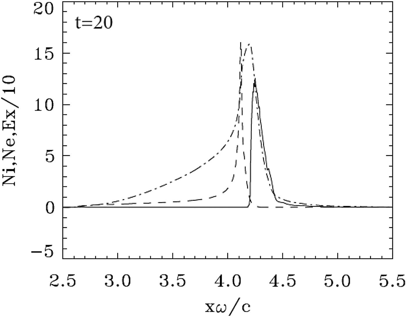
Fig. 10. Electron (full curves) and ion (dashed curves) density profiles for case 3 (a 0 = 100). The electric field (dashed-dotted curves divided by a factor of 10). The plot is at time t = 20.0.
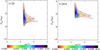
Fig. 11. Phase-space plots of the electron distribution function for case 3 (a 0 = 100). The plots are at times: t = 20 and 20.8. Note the ejection of the electrons to the right, and the acceleration of the electron cloud.

Fig. 12. Incident wave E + (full curve) and reflected wave E − (dashed curve) at t = 21.6 and 22.4 for case 3 (a 0 = 100). Note the penetration of the incident laser beam (full curve) across the target.
5. CONCLUSION
We have used an Eulerian Vlasov code for the numerical solution of the 1D relativistic Vlasov–Maxwell equations to study the interaction of an ultra-short high-intensity circularly polarized laser beam normally incident on a target, at a critical thickness of the target: first when the target is opaque to the laser beam and the laser pulse does not penetrate the target (the case with a 0 = 80), then when there is a very small penetration of the laser pulse through the target (the second case with a 0 = 90), and a third case where there is a more important penetration of the laser pulse through the target (a 0 = 100), which was dealt with in Shoucri et al. (Reference Shoucri, Matte and Vidal2016). In the three cases, a high density target with n/n cr = 100 is considered. For the first two cases considered, the ponderomotive force or radiation pressure has the dominant role, although the phase-space evolution of the electron distribution function is totally different. Initially the electrons are pushed by the radiation pressure, and form a steep gradient at the target surface. This generates a charge separation and an electric field at the plasma edge, which accelerates the ions. Under the effect of the radiation pressure acting on the electron surface, the ion peak and the electron peak separate, and the whole thin foil has been transformed into a double-layer structure. The radiative pressure acceleration is acting on the double layer as a whole [very close to what is described in Fig. 1 in Schlegel et al. (Reference Schlegel, Naumova, Tikhonchuk, Labaune, Sokolov and Mourou2009), in Fig. 2 of Eliezer et al. (Reference Eliezer, Nissim, Martinez-Val, Mima and Hora2014) and in Shoucri et al. (Reference Shoucri, Matte and Vidal2016)], with an electric field between the two peaks providing a restoring force. In the second case, however, there is an electron population leaking in the forward direction, which develops a spiral structure in the phase space, and results in the sawtooth structure of the electron density profile we observe in Figure 6 [see also Shoucri et al. (Reference Shoucri, Matte and Vidal2013, Reference Shoucri, Matte and Vidal2014)]. Eventually an ion population develops inside the electron layer forming a quasi-neutral plasma jet. We then observe an electron peak containing the excess electron population, which splits from the forward propagating neutral plasma jet and decelerates due to the decaying radiation pressure of the laser pulse and the space-charge electric field. Compared with the results of the first case, a 27% increase in intensity gives a 69% increase in ion energy. The ion group in the neutral plasma bunch travels at the constant speed, which it acquired during the laser pulse.
By contrast, we noted in the third case with a 0 = 100 that a fraction of the laser pulse is transmitted through the target, and the entire electron population forms a cloud, which is accelerated and completely expelled from the back of the target. Scisciò et al. (Reference Scisciò, d'Humières, Fourmaux, Kieffer, Palumbo and Antici2014) and d'Humières et al. (Reference d'Humières, Lefebvre, Gremillet and Malka2005, Reference d'Humières, Brantov, Bychenkov and Tikhonchuk2013) for instance have discussed the features of proton acceleration with high-intensity lasers as a function of target thickness, where below a given thickness a fraction of the laser energy is transmitted through the target. This thickness delimits two regimes of acceleration: the opaque and the transparent regimes. The former corresponds to the first case we have studied, where the wave does not penetrate through the target, the latter to the transparent regime we studied in the third case. There is however between these two cases a case where there is a weak penetration of the laser pulse through the target. In this case, the evolution of the electron distribution function is totally different from the two other cases, and shows the development of spiral structure in the phase space and the appearance of sawtooth modulations on the electron density profiles (Shoucri et al., Reference Shoucri, Matte and Vidal2013, Reference Shoucri, Matte and Vidal2014).
With the precision of the Vlasov code, the present study provides more insight in the evolution of the phase-space structures of the electron distribution functions, which is different in the three cases. A main feature presented in the present work is in the transition between the opaque regime and the transparent regime, when a very small fraction of the laser pulse penetrates through the target. The Vlasov code shows in the second simulation the details of the spiral structure, which develops in the phase space of the electron distribution function, before leading to the final neutral plasma jet.
Acknowledgements
M. Shoucri is grateful to Dr Réjean Girard for his constant interest. The authors are grateful to the Centre de Calcul Scientifique de l'IREQ (CASIR) for the computer time used in the simulations presented in the present work.


