


1 Introduction
The physical understanding of the turbulence dynamics of dense gas flows is relevant for several engineering systems, such as high-Reynolds-number wind tunnels (Anderson Reference Anderson1991), chemical transport and processing (Kirillov Reference Kirillov2004), energy conversion cycles (Monaco, Cramer & Watson Reference Monaco, Cramer and Watson1997; Brown & Argrow Reference Brown and Argrow2000; Horen et al. Reference Horen, Talonpoika, Larjola and Siikonen2002) and refrigeration (Zamfirescu & Dincer Reference Zamfirescu and Dincer2009).
Dense gases are single-phase fluids characterized by high molecular complexity and moderate to large molecular weights. The dynamics of dense gases is described by the fundamental derivative of gas dynamics (Thompson Reference Thompson1971)
 $$\begin{eqnarray}\unicode[STIX]{x1D6E4}=1+\frac{\unicode[STIX]{x1D70C}}{c}\left.\frac{\unicode[STIX]{x2202}c}{\unicode[STIX]{x2202}\unicode[STIX]{x1D70C}}\right|_{s},\end{eqnarray}$$
(where
 $\unicode[STIX]{x1D70C}$
is the density,
$\unicode[STIX]{x1D70C}$
is the density,
 $p$
the pressure,
$p$
the pressure,
 $s$
the entropy and
$s$
the entropy and
 $c$
the sound speed), which measures the rate of change of the sound speed in isentropic transformations. In a range of thermodynamic conditions next to the saturation curve, the value of
$c$
the sound speed), which measures the rate of change of the sound speed in isentropic transformations. In a range of thermodynamic conditions next to the saturation curve, the value of
 $\unicode[STIX]{x1D6E4}$
can be less than one or even negative. In such conditions, the sound speed increases in isentropic expansions and decreases in isentropic compressions, unlike the case of perfect gases (PFGs). Dense gas effects are expected to give the most interesting phenomena for a family of heavy polyatomic compounds, named Bethe–Zel’dovich–Thompson (BZT) fluids (Bethe Reference Bethe1942; Zel’Dovich & Raizer Reference Zel’Dovich and Raizer1966; Thompson Reference Thompson1971), which exhibit a region of negative
$\unicode[STIX]{x1D6E4}$
can be less than one or even negative. In such conditions, the sound speed increases in isentropic expansions and decreases in isentropic compressions, unlike the case of perfect gases (PFGs). Dense gas effects are expected to give the most interesting phenomena for a family of heavy polyatomic compounds, named Bethe–Zel’dovich–Thompson (BZT) fluids (Bethe Reference Bethe1942; Zel’Dovich & Raizer Reference Zel’Dovich and Raizer1966; Thompson Reference Thompson1971), which exhibit a region of negative
 $\unicode[STIX]{x1D6E4}$
values (called the ‘inversion zone’, see Cramer & Kluwick Reference Cramer and Kluwick1984) in the vapour phase close to the liquid/vapour coexistence curve. This is theoretically predicted to result in non-classical compressibility effects in the transonic and supersonic flow regimes, like rarefaction shock waves, mixed shock/fan waves and shock splitting (see e.g. Cramer & Kluwick Reference Cramer and Kluwick1984; Cramer Reference Cramer1989b
, Reference Cramer1991; Rusak & Wang Reference Rusak and Wang1997). Furthermore, the entropy change across a weak shock, given by (Bethe Reference Bethe1942)
$\unicode[STIX]{x1D6E4}$
values (called the ‘inversion zone’, see Cramer & Kluwick Reference Cramer and Kluwick1984) in the vapour phase close to the liquid/vapour coexistence curve. This is theoretically predicted to result in non-classical compressibility effects in the transonic and supersonic flow regimes, like rarefaction shock waves, mixed shock/fan waves and shock splitting (see e.g. Cramer & Kluwick Reference Cramer and Kluwick1984; Cramer Reference Cramer1989b
, Reference Cramer1991; Rusak & Wang Reference Rusak and Wang1997). Furthermore, the entropy change across a weak shock, given by (Bethe Reference Bethe1942)
 $$\begin{eqnarray}\unicode[STIX]{x0394}s=-\frac{c^{2}\unicode[STIX]{x1D6E4}}{v^{3}}\frac{(\unicode[STIX]{x0394}v)^{3}}{6T}+O((\unicode[STIX]{x0394}v)^{4}),\end{eqnarray}$$
with
 $T$
the absolute temperature, is much weaker than usual for dense gases with
$T$
the absolute temperature, is much weaker than usual for dense gases with
 $\unicode[STIX]{x1D6E4}\leqslant 1$
, leading to reduced shock losses. The reader may refer, e.g., to Cinnella & Congedo (Reference Cinnella and Congedo2007) and references cited therein for more details.
$\unicode[STIX]{x1D6E4}\leqslant 1$
, leading to reduced shock losses. The reader may refer, e.g., to Cinnella & Congedo (Reference Cinnella and Congedo2007) and references cited therein for more details.
For dense gases, the PFG model is no longer valid, and more complex equations of state (EoS) are used to account for their peculiar thermodynamic behaviour. The Van der Waals EoS (Van der Waals Reference Van der Waals1873), which takes into account the co-volume occupied by the molecules and the two-body collision interactions, is the simplest gas model accounting for dense gas effects, including the qualitative features of BZT flows, but it is not very accurate for thermodynamic conditions close to saturation, and largely over-predicts the extent of the inversion zone (Thompson & Lambrakis Reference Thompson and Lambrakis1973). A more accurate representation of the fluid properties can be achieved by using a more complex cubic EoS such as the Peng–Robinson–Stryjeck–Vera (Stryjek & Vera Reference Stryjek and Vera1986) EoS, a virial-expansion EoS such as the Martin–Hou (Martin & Hou Reference Martin and Hou1955) EoS or multiparameter models based e.g. on Helmoltz’ free energy (Lemmon & Span Reference Lemmon and Span2006).
A second important consideration is that in the dense gas regime, the dynamic viscosity
 $\unicode[STIX]{x1D707}$
and the thermal conductivity
$\unicode[STIX]{x1D707}$
and the thermal conductivity
 $\unicode[STIX]{x1D705}$
depend both on temperature and pressure through complex relationships. In this respect, the dense gas regime is a transition between two qualitatively different behaviours, namely, the one of liquids, whose viscosity tends to decrease with increasing temperature, and that of dilute gases, for which it increases with
$\unicode[STIX]{x1D705}$
depend both on temperature and pressure through complex relationships. In this respect, the dense gas regime is a transition between two qualitatively different behaviours, namely, the one of liquids, whose viscosity tends to decrease with increasing temperature, and that of dilute gases, for which it increases with
 $T$
. Additionally, in the dense gas region the dependency of
$T$
. Additionally, in the dense gas region the dependency of
 $\unicode[STIX]{x1D707}$
and
$\unicode[STIX]{x1D707}$
and
 $\unicode[STIX]{x1D705}$
on the fluid pressure (or density) is no longer negligible (Chung et al.
Reference Chung, Ajlan, Lee and Starling1988). Finally, the classical approximation of nearly constant Prandtl number (
$\unicode[STIX]{x1D705}$
on the fluid pressure (or density) is no longer negligible (Chung et al.
Reference Chung, Ajlan, Lee and Starling1988). Finally, the classical approximation of nearly constant Prandtl number (
 $Pr=\unicode[STIX]{x1D707}c_{p}/\unicode[STIX]{x1D705}\approx$
const.) is no longer valid. In particular, the thermal conductivity varies as the viscosity with temperature and pressure, and the behaviour of
$Pr=\unicode[STIX]{x1D707}c_{p}/\unicode[STIX]{x1D705}\approx$
const.) is no longer valid. In particular, the thermal conductivity varies as the viscosity with temperature and pressure, and the behaviour of
 $Pr$
tends to be controlled by variations of
$Pr$
tends to be controlled by variations of
 $c_{p}$
. Hence, in regions where
$c_{p}$
. Hence, in regions where
 $c_{p}$
becomes large, strong variations of
$c_{p}$
becomes large, strong variations of
 $Pr$
are expected, contrary to what occurs in PFGs. However, the Prandtl number remains of order one except in the immediate vicinity of the thermodynamic critical point, where it can attain very large values. In contrast, the Eckert number (
$Pr$
are expected, contrary to what occurs in PFGs. However, the Prandtl number remains of order one except in the immediate vicinity of the thermodynamic critical point, where it can attain very large values. In contrast, the Eckert number (
 $Ec=U_{0}^{2}/2\,c_{p_{0}}T_{0}$
, defined at a suitable reference state with velocity
$Ec=U_{0}^{2}/2\,c_{p_{0}}T_{0}$
, defined at a suitable reference state with velocity
 $U_{0}$
, temperature
$U_{0}$
, temperature
 $T_{0}$
and isobaric specific heat
$T_{0}$
and isobaric specific heat
 $c_{p_{0}}$
), which is a measure of the sensitivity to friction heating, is significantly lower than in PFGs.
$c_{p_{0}}$
), which is a measure of the sensitivity to friction heating, is significantly lower than in PFGs.
The present paper aims to investigate the influence of dense gases governed by a complex EoS on the turbulence dynamics. Numerical simulations of turbulent dense gas flows and specifically those based on the Reynolds-averaged Navier–Stokes (RANS) equations are in high demand, in particular for turbomachinery applications (e.g. Harinck et al. Reference Harinck, Turunen-Saaresti, Colonna, Rebay and van Buijtenen2010; Wheeler & Ong Reference Wheeler and Ong2013, Reference Wheeler and Ong2014; Sciacovelli & Cinnella Reference Sciacovelli and Cinnella2014). However, the accuracy of RANS models for these flows has not been properly assessed up to now due to the lack of reference data either experimental or numerical. Reliable and complete direct numerical simulation (DNS) databases are then needed to quantify the deficiencies of existing turbulence models and provide a database for the development and calibration of improved models.
For PFGs at sufficiently high turbulent Mach numbers, turbulence is strongly affected by randomly distributed spatially varying shocks (referred to as shocklets) and other compressibility effects. Shocklet formation was discussed by Passot & Pouquet (Reference Passot and Pouquet1987) and Lee, Lele & Moin (Reference Lee, Lele and Moin1991). Erlebacher & Sarkar (Reference Erlebacher and Sarkar1993) carried out DNS of compressible homogeneous shear flow turbulence and highlighted the differences in the behaviour of the solenoidal and irrotational strain-rate tensors. Samtaney, Pullin & Kosovic (Reference Samtaney, Pullin and Kosovic2001) presented DNS of decaying compressible homogeneous isotropic turbulence (CHIT) for initial turbulent Mach numbers (
 $M_{t_{0}}$
) comprised in the range 0.1–0.5 and Reynolds numbers based on the Taylor microscale (
$M_{t_{0}}$
) comprised in the range 0.1–0.5 and Reynolds numbers based on the Taylor microscale (
 $Re_{\unicode[STIX]{x1D706}}$
) in the range 50–100. They developed an algorithm to extract and quantify the shocklet statistics from the DNS fields, pointed out the appearance of random shocklets during the main part of the decay and showed that the shock thickness statistics scale with the Kolmogorov length. The statistical properties of decaying CHIT were analysed by Pirozzoli & Grasso (Reference Pirozzoli and Grasso2004) for various turbulent Mach numbers. Those authors discussed the influence of compressibility on the time evolution of mean turbulence properties and on the statistical properties and dynamics of turbulent structures. Specifically they found that the joint probability density function (p.d.f.) of the second and third invariants of the anisotropic part of the deformation-rate tensor has a universal teardrop shape, as in incompressible turbulence. They also confirmed that, due to the competing mechanisms of vortex stretching and viscous dissipation, the enstrophy obeys a two-stage evolution; however, at high turbulent Mach numbers, compressibility effects associated with the occurrence of shocklets become important. The effects of local compressibility on the statistical properties and structures of velocity gradients for forced CHIT at high turbulent Mach number were studied by Wang et al. (Reference Wang, Shi, Wang, Xiao, He and Chen2012). Those authors showed in particular that strong local compression motions enhance the enstrophy production by vortex stretching, while strong local expansion motions suppress enstrophy through the same mechanism. Jagannathan & Donzis (Reference Jagannathan and Donzis2016) also studied stochastically forced CHIT at various Reynolds and Mach numbers. They suggested that for turbulent Mach number above a critical value of approximately 0.3, dilatational effects strongly influence the flow behaviour. Specifically, strong compressions were found to be ten times more likely than strong expansions at high Mach numbers, resulting in significant changes in the dynamics of energy exchanges. Furthermore, the probability distribution of local dilatation was shown to develop long negative tails (thus leading to a negative skewness).
$Re_{\unicode[STIX]{x1D706}}$
) in the range 50–100. They developed an algorithm to extract and quantify the shocklet statistics from the DNS fields, pointed out the appearance of random shocklets during the main part of the decay and showed that the shock thickness statistics scale with the Kolmogorov length. The statistical properties of decaying CHIT were analysed by Pirozzoli & Grasso (Reference Pirozzoli and Grasso2004) for various turbulent Mach numbers. Those authors discussed the influence of compressibility on the time evolution of mean turbulence properties and on the statistical properties and dynamics of turbulent structures. Specifically they found that the joint probability density function (p.d.f.) of the second and third invariants of the anisotropic part of the deformation-rate tensor has a universal teardrop shape, as in incompressible turbulence. They also confirmed that, due to the competing mechanisms of vortex stretching and viscous dissipation, the enstrophy obeys a two-stage evolution; however, at high turbulent Mach numbers, compressibility effects associated with the occurrence of shocklets become important. The effects of local compressibility on the statistical properties and structures of velocity gradients for forced CHIT at high turbulent Mach number were studied by Wang et al. (Reference Wang, Shi, Wang, Xiao, He and Chen2012). Those authors showed in particular that strong local compression motions enhance the enstrophy production by vortex stretching, while strong local expansion motions suppress enstrophy through the same mechanism. Jagannathan & Donzis (Reference Jagannathan and Donzis2016) also studied stochastically forced CHIT at various Reynolds and Mach numbers. They suggested that for turbulent Mach number above a critical value of approximately 0.3, dilatational effects strongly influence the flow behaviour. Specifically, strong compressions were found to be ten times more likely than strong expansions at high Mach numbers, resulting in significant changes in the dynamics of energy exchanges. Furthermore, the probability distribution of local dilatation was shown to develop long negative tails (thus leading to a negative skewness).
In a previous paper, the present authors have investigated the influence of dense gases on the large-scale dynamics of decaying CHIT in the limit of
 $Re\rightarrow \infty$
by using an inviscid flow model (Sciacovelli et al.
Reference Sciacovelli, Cinnella, Content and Grasso2016). A thorough parametric study was conducted based on the Van der Waals gas model, with focus on dense gases of the BZT type. Dense gas effects were found to have a significant influence on the time evolution of the root mean square (r.m.s.) of the thermodynamic properties (namely, density, pressure and speed of sound) for flows characterized by sufficiently high initial turbulent Mach numbers (above 0.5), whereas the influence on kinematic properties, such as the kinetic energy and the vorticity, was found to be smaller. However, the flow dilatational behaviour was found to be deeply different, due to the non-classical variation of the speed of sound in flow regions where the dense gas is characterized by values of the fundamental derivative of gas dynamics smaller than one or even negative. The most significant differences between the perfect and the dense gas case were observed for the repartition of dilatation levels in the flow field. For the PFG, strong compression regions (where compression shocklets may occur) exhibit sheet-like structures and occupy a much larger volume fraction than expansion regions, which are instead characterized by tubular structures. Accordingly, the probability distributions of the velocity divergence is highly skewed toward negative values. For the dense gas case, the volume fractions occupied by strong expansion and compression regions were much more balanced, and characterized by a sheet-like topology. This led the authors to conclude that expansion eddy shocklets may appear in the dense gas.
$Re\rightarrow \infty$
by using an inviscid flow model (Sciacovelli et al.
Reference Sciacovelli, Cinnella, Content and Grasso2016). A thorough parametric study was conducted based on the Van der Waals gas model, with focus on dense gases of the BZT type. Dense gas effects were found to have a significant influence on the time evolution of the root mean square (r.m.s.) of the thermodynamic properties (namely, density, pressure and speed of sound) for flows characterized by sufficiently high initial turbulent Mach numbers (above 0.5), whereas the influence on kinematic properties, such as the kinetic energy and the vorticity, was found to be smaller. However, the flow dilatational behaviour was found to be deeply different, due to the non-classical variation of the speed of sound in flow regions where the dense gas is characterized by values of the fundamental derivative of gas dynamics smaller than one or even negative. The most significant differences between the perfect and the dense gas case were observed for the repartition of dilatation levels in the flow field. For the PFG, strong compression regions (where compression shocklets may occur) exhibit sheet-like structures and occupy a much larger volume fraction than expansion regions, which are instead characterized by tubular structures. Accordingly, the probability distributions of the velocity divergence is highly skewed toward negative values. For the dense gas case, the volume fractions occupied by strong expansion and compression regions were much more balanced, and characterized by a sheet-like topology. This led the authors to conclude that expansion eddy shocklets may appear in the dense gas.
We observe that the Van der Waals model provides a good qualitative description of dense gas and BZT effects. However, it does not provide an accurate representation of the fluid behaviour; it is then important to investigate the robustness of the observed effects for other gas models. Additionally, a detailed investigation of the effects of eddy shocklets requires an analysis of the small-scale behaviour that is governed by viscous effects.
In the present paper, we focus on the role of viscous effects involved in the small-scale dynamics of dense gas CHIT. On the one hand, we investigate how differences due to the complex thermodynamic behaviour affect the dynamics at the smallest scales. On the other hand, we elucidate the role of the peculiar transport properties of dense gases. With this aim, we carry out DNS of the compressible Navier–Stokes equations for dense gases governed by complex EoS and transport laws. We focus in particular on flows of perfluoro-perhydrophenanthrene (chemical formula C
 $_{14}$
F
$_{14}$
F
 $_{24}$
, called hereafter by its commercial name PP11), a heavy fluorocarbon gas that has been extensively studied in the dense gas literature (e.g. Cramer & Tarkenton Reference Cramer and Tarkenton1992; Monaco et al.
Reference Monaco, Cramer and Watson1997; Guardone & Argrow Reference Guardone and Argrow2005; Sciacovelli et al.
Reference Sciacovelli, Cinnella, Content and Grasso2016). The thermodynamic behaviour of the gas is described by means of the Martin–Hou EoS that represents a reasonably accurate model for fluorocarbons, and an accurate dense gas formulation is used to determine the transport properties (Chung et al.
Reference Chung, Ajlan, Lee and Starling1988). Simulations are carried out at various initial turbulent Mach numbers and for two different choices of the initial thermodynamic state, corresponding to a small positive and a small negative value of the fundamental derivative
$_{24}$
, called hereafter by its commercial name PP11), a heavy fluorocarbon gas that has been extensively studied in the dense gas literature (e.g. Cramer & Tarkenton Reference Cramer and Tarkenton1992; Monaco et al.
Reference Monaco, Cramer and Watson1997; Guardone & Argrow Reference Guardone and Argrow2005; Sciacovelli et al.
Reference Sciacovelli, Cinnella, Content and Grasso2016). The thermodynamic behaviour of the gas is described by means of the Martin–Hou EoS that represents a reasonably accurate model for fluorocarbons, and an accurate dense gas formulation is used to determine the transport properties (Chung et al.
Reference Chung, Ajlan, Lee and Starling1988). Simulations are carried out at various initial turbulent Mach numbers and for two different choices of the initial thermodynamic state, corresponding to a small positive and a small negative value of the fundamental derivative
 $\unicode[STIX]{x1D6E4}$
, and the results are compared with PFG ones.
$\unicode[STIX]{x1D6E4}$
, and the results are compared with PFG ones.
The paper is organized as follows. Section 2 recalls the governing equations, the closure models adopted to describe the thermodynamic and transport properties of the dense gas and provides a description of the numerical methodology. Section 3 discusses the time evolution of the general statistics of the flow field at various initial turbulent Mach numbers, with specific focus on thermodynamic variables and on flow properties of particular relevance in compressible flows, such as the dilatation. In § 4 we analyse the flow topology according to the invariants of the deviatoric strain-rate tensor and identify the structure types associated with compressing and expanding regions. Finally, § 5 sheds further light on the underlying dissipation mechanisms in dense gas turbulence by analysing the contribution of flow structures to enstrophy generation.
2 Formulation and numerical methodology
2.1 Governing equations and approximation schemes
In the present study we consider flows of gases in the single-phase regime, governed by the compressible Navier–Stokes equations that are written in differential form
 $$\begin{eqnarray}\displaystyle & \displaystyle \frac{\unicode[STIX]{x2202}\unicode[STIX]{x1D70C}}{\unicode[STIX]{x2202}t}+\frac{\unicode[STIX]{x2202}(\unicode[STIX]{x1D70C}u_{j})}{\unicode[STIX]{x2202}x_{j}}=0 & \displaystyle\end{eqnarray}$$
 $$\begin{eqnarray}\displaystyle & \displaystyle \frac{\unicode[STIX]{x2202}\unicode[STIX]{x1D70C}u_{i}}{\unicode[STIX]{x2202}t}+\frac{\unicode[STIX]{x2202}(\unicode[STIX]{x1D70C}u_{i}u_{j})}{\unicode[STIX]{x2202}x_{j}}=-\frac{\unicode[STIX]{x2202}p}{\unicode[STIX]{x2202}x_{i}}+\frac{\unicode[STIX]{x2202}\unicode[STIX]{x1D70E}_{ij}}{\unicode[STIX]{x2202}x_{j}} & \displaystyle\end{eqnarray}$$
 $$\begin{eqnarray}\displaystyle & \displaystyle \frac{\unicode[STIX]{x2202}\unicode[STIX]{x1D70C}E}{\unicode[STIX]{x2202}t}+\frac{\unicode[STIX]{x2202}((\unicode[STIX]{x1D70C}E+p)u_{j})}{\unicode[STIX]{x2202}x_{j}}=\frac{\unicode[STIX]{x2202}(\unicode[STIX]{x1D70E}_{ij}u_{i})}{\unicode[STIX]{x2202}x_{j}}-\frac{\unicode[STIX]{x2202}q_{j}}{\unicode[STIX]{x2202}x_{j}}, & \displaystyle\end{eqnarray}$$
with
 $u_{i}$
the velocity vector components,
$u_{i}$
the velocity vector components,
 $\unicode[STIX]{x1D70C}$
the density and
$\unicode[STIX]{x1D70C}$
the density and
 $p$
the pressure. The specific total energy
$p$
the pressure. The specific total energy
 $E$
and the viscous stress tensor
$E$
and the viscous stress tensor
 $\unicode[STIX]{x1D70E}_{ij}$
are given by
$\unicode[STIX]{x1D70E}_{ij}$
are given by
 $$\begin{eqnarray}\displaystyle & \displaystyle E\equiv e+{\textstyle \frac{1}{2}}u_{j}u_{j} & \displaystyle\end{eqnarray}$$
 $$\begin{eqnarray}\displaystyle & \displaystyle \unicode[STIX]{x1D70E}_{ij}\equiv \unicode[STIX]{x1D707}\left(\frac{\unicode[STIX]{x2202}u_{i}}{\unicode[STIX]{x2202}x_{j}}+\frac{\unicode[STIX]{x2202}u_{j}}{\unicode[STIX]{x2202}x_{i}}\right)-\frac{2}{3}\unicode[STIX]{x1D707}\unicode[STIX]{x1D703}\unicode[STIX]{x1D6FF}_{ij}, & \displaystyle\end{eqnarray}$$
where
 $e$
is the specific internal energy,
$e$
is the specific internal energy,
 $\unicode[STIX]{x1D707}$
the dynamic viscosity,
$\unicode[STIX]{x1D707}$
the dynamic viscosity,
 $\unicode[STIX]{x1D703}\equiv \unicode[STIX]{x2202}u_{k}/\unicode[STIX]{x2202}x_{k}$
the dilatation,
$\unicode[STIX]{x1D703}\equiv \unicode[STIX]{x2202}u_{k}/\unicode[STIX]{x2202}x_{k}$
the dilatation,
 $\unicode[STIX]{x1D6FF}_{ij}$
the Kronecker delta and where we have used the well-known Stokes’ hypothesis in neglecting the contribution of the bulk viscosity, which is a widely accepted approximation for most flows and namely for air flows. The study of Cramer (Reference Cramer2012) provides some numerical estimates for the bulk viscosity of ideal gases. It shows that the latter can vary significantly with the temperature and can be as large as hundreds or thousands of times the shear viscosity, even for some common diatomic gases. Nevertheless, its effect, additive to that of the thermodynamic pressure, is generally several orders of magnitude smaller. Its contribution is then expected to be negligible except, possibly, in very high dilatation regions such as the locations of shocklets where it may introduce an additional damping. For more complex gases, bulk viscosity data are even scarcer. Based on the preceding arguments, we will neglect its contribution also for dense gas flows.
$\unicode[STIX]{x1D6FF}_{ij}$
the Kronecker delta and where we have used the well-known Stokes’ hypothesis in neglecting the contribution of the bulk viscosity, which is a widely accepted approximation for most flows and namely for air flows. The study of Cramer (Reference Cramer2012) provides some numerical estimates for the bulk viscosity of ideal gases. It shows that the latter can vary significantly with the temperature and can be as large as hundreds or thousands of times the shear viscosity, even for some common diatomic gases. Nevertheless, its effect, additive to that of the thermodynamic pressure, is generally several orders of magnitude smaller. Its contribution is then expected to be negligible except, possibly, in very high dilatation regions such as the locations of shocklets where it may introduce an additional damping. For more complex gases, bulk viscosity data are even scarcer. Based on the preceding arguments, we will neglect its contribution also for dense gas flows.
Finally,
 $q_{j}$
represents the heat flux, modelled by means of Fourier’s law:
$q_{j}$
represents the heat flux, modelled by means of Fourier’s law:
 $$\begin{eqnarray}q_{j}=-\unicode[STIX]{x1D705}\frac{\unicode[STIX]{x2202}T}{\unicode[STIX]{x2202}x_{j}},\end{eqnarray}$$
where
 $\unicode[STIX]{x1D705}$
is the thermal conductivity. The system is supplemented by thermal and caloric equations of state, respectively:
$\unicode[STIX]{x1D705}$
is the thermal conductivity. The system is supplemented by thermal and caloric equations of state, respectively:
 $$\begin{eqnarray}p=p(\unicode[STIX]{x1D70C},T)\quad \text{and}\quad e=e(\unicode[STIX]{x1D70C},T).\end{eqnarray}$$
These equations satisfy the compatibility relation:
 $$\begin{eqnarray}e=e_{\mathit{ref}}+\int _{T_{\mathit{ref}}}^{T}c_{v,\infty }(T)\,\text{d}T-\int _{\unicode[STIX]{x1D70C}_{\mathit{ref}}}^{\unicode[STIX]{x1D70C}}\left[T\left.\frac{\unicode[STIX]{x2202}p}{\unicode[STIX]{x2202}T}\right|_{\unicode[STIX]{x1D70C}}-p\right]\frac{\text{d}\unicode[STIX]{x1D70C}}{\unicode[STIX]{x1D70C}^{2}},\end{eqnarray}$$
where the subscript
 $(\cdot )_{\mathit{ref}}$
indicates a reference state, and
$(\cdot )_{\mathit{ref}}$
indicates a reference state, and
 $c_{v,\infty }(T)$
is the isochoric specific heat in the ideal gas limit.
$c_{v,\infty }(T)$
is the isochoric specific heat in the ideal gas limit.
In the present work, the gas behaviour is modelled through the Martin–Hou thermal equation of state (Martin & Hou Reference Martin and Hou1955). Such a model involves five virial terms and satisfies ten thermodynamic constraints, and it ensures high accuracy with a minimum of experimental information, thus providing a realistic description of the gas behaviour and of the inversion zone size. The equation reads
 $$\begin{eqnarray}p=\frac{RT}{v-b}+\mathop{\sum }_{i=2}^{5}\frac{f_{i}(T)}{(v-b)^{i}},\end{eqnarray}$$
where
 $v\equiv 1/\unicode[STIX]{x1D70C}$
is the specific volume,
$v\equiv 1/\unicode[STIX]{x1D70C}$
is the specific volume,
 $R={\mathcal{R}}/{\mathcal{M}}$
is the gas constant (with
$R={\mathcal{R}}/{\mathcal{M}}$
is the gas constant (with
 ${\mathcal{R}}$
the universal gas constant and
${\mathcal{R}}$
the universal gas constant and
 ${\mathcal{M}}$
the molecular weight),
${\mathcal{M}}$
the molecular weight),
 $b$
is the co-volume occupied by the fluid molecules and the functions
$b$
is the co-volume occupied by the fluid molecules and the functions
 $f_{i}(T)$
are of the form
$f_{i}(T)$
are of the form
 $$\begin{eqnarray}f_{i}(T)=A_{i}+B_{i}T+C_{i}\text{e}^{-k(T/T_{c})},\end{eqnarray}$$
with
 $T_{c}$
the critical temperature and
$T_{c}$
the critical temperature and
 $k=5.475$
. The gas-dependent coefficients
$k=5.475$
. The gas-dependent coefficients
 $A_{i}$
,
$A_{i}$
,
 $B_{i}$
,
$B_{i}$
,
 $C_{i}$
can be expressed in terms of the critical temperature and pressure, the critical compressibility factor, the Boyle temperature and one point on the vapour pressure curve. A power law of the form
$C_{i}$
can be expressed in terms of the critical temperature and pressure, the critical compressibility factor, the Boyle temperature and one point on the vapour pressure curve. A power law of the form
 $$\begin{eqnarray}c_{v_{\infty }}=c_{v_{\infty }}(T_{c})\left(\frac{T}{T_{c}}\right)^{n}\end{eqnarray}$$
is used to model variations of the low-density specific heat with temperature, where
 $n$
is a parameter that depends on the gas used (for more details, see Cramer Reference Cramer1989a
). The viscosity and thermal conductivity have been modelled according to the accurate dense gas formulation of Chung, Lee & Starling (Reference Chung, Lee and Starling1984), Chung et al. (Reference Chung, Ajlan, Lee and Starling1988), also described in the book of Poling et al. (Reference Poling, Prausnitz, O’Connell and Reid2001).
$n$
is a parameter that depends on the gas used (for more details, see Cramer Reference Cramer1989a
). The viscosity and thermal conductivity have been modelled according to the accurate dense gas formulation of Chung, Lee & Starling (Reference Chung, Lee and Starling1984), Chung et al. (Reference Chung, Ajlan, Lee and Starling1988), also described in the book of Poling et al. (Reference Poling, Prausnitz, O’Connell and Reid2001).
In the following, simulations are carried out considering PP11 as the working fluid, whose thermodynamic properties are provided in table 1. This gas has been often used in the dense gas literature because it is predicted to exhibit a relatively wide inversion zone and, as a consequence, BZT effects.
Table 1. Thermodynamic properties of PP11: molecular weight (
 ${\mathcal{M}}$
), critical temperature (
${\mathcal{M}}$
), critical temperature (
 $T_{c}$
), critical density (
$T_{c}$
), critical density (
 $\unicode[STIX]{x1D70C}_{c}$
), critical pressure (
$\unicode[STIX]{x1D70C}_{c}$
), critical pressure (
 $p_{c}$
), critical compressibility factor (
$p_{c}$
), critical compressibility factor (
 $Z_{c}$
), acentric factor (
$Z_{c}$
), acentric factor (
 $\unicode[STIX]{x1D714}_{ac}$
), dipole moment (
$\unicode[STIX]{x1D714}_{ac}$
), dipole moment (
 $\unicode[STIX]{x1D709}$
) of the gas phase, boiling temperature (
$\unicode[STIX]{x1D709}$
) of the gas phase, boiling temperature (
 $T_{b}$
), ratio of ideal gas specific heat at constant volume over the gas constant (
$T_{b}$
), ratio of ideal gas specific heat at constant volume over the gas constant (
 $c_{v}(T_{c})/R$
) at the critical point and exponent of the power law for the low-density specific heat (
$c_{v}(T_{c})/R$
) at the critical point and exponent of the power law for the low-density specific heat (
 $n$
).
$n$
).

The numerical strategy relies on a fourth-order discretization, whereby the convective terms are approximated by optimized finite differences with an eleven-point stencil in each mesh direction (Bogey & Bailly Reference Bogey and Bailly2004) and the viscous terms are approximated by fourth-order central differences. To damp grid-to-grid oscillations in smooth flow regions, an optimized selective sixth-order filter based on an eleven-point stencil is applied in each direction. In order to ensure computational robustness across flow discontinuities, an adaptive nonlinear selective filtering strategy similar to that of Bogey, De Cacqueray & Bailly (Reference Bogey, De Cacqueray and Bailly2009) is employed. In particular, to avoid the appearance of spurious oscillations, a low-order filter based on a Ducros-type shock sensor (Ducros et al. Reference Ducros, Ferrand, Nicoud, Weber, Darracq, Gacherieu and Poinsot1999) is introduced. The sensor triggers the required additional damping in regions characterized by high dilatation levels compared with the local vorticity magnitude, while it is not active in regions where the flow is smooth or dominated by vortical structures (see Bogey et al. Reference Bogey, De Cacqueray and Bailly2009 for details). A low-storage six-stage Runge–Kutta scheme optimized in the wavenumber space (Bogey & Bailly Reference Bogey and Bailly2004) is used for time integration. The adaptive filter is applied at the last stage of the Runge–Kutta integration. The preceding numerical strategy has been widely demonstrated for direct and large eddy simulations of compressible flows with and without shocks (see, e.g., Bogey & Bailly Reference Bogey and Bailly2009; Bogey, Marsden & Bailly Reference Bogey, Marsden and Bailly2012; Aubard, Gloerfelt & Robinet Reference Aubard, Gloerfelt and Robinet2013; Gloerfelt & Berland Reference Gloerfelt and Berland2013). Validations of the present DNS code against results in the literature are reported in appendix A.
2.2 Initial conditions
The CHIT decay problem is solved in the cubic domain
 $[0,2\unicode[STIX]{x03C0}]^{3}$
, and periodic boundary conditions are applied in the three directions.
$[0,2\unicode[STIX]{x03C0}]^{3}$
, and periodic boundary conditions are applied in the three directions.
The issue of the initial conditions for compressible isotropic turbulence has been addressed by various authors (Blaisdell, Mansour & Reynolds Reference Blaisdell, Mansour and Reynolds1993; Ristorcelli & Blaisdell Reference Ristorcelli and Blaisdell1997; Samtaney et al.
Reference Samtaney, Pullin and Kosovic2001). In general, the shape of the initial three-dimensional spectrum and the root-mean-square (r.m.s.) level of each flow variable must be provided. Furthermore, different spectra can be assigned to the solenoidal and dilatational components. The main difference between an incompressible and compressible initialization is the presence of an intrinsic velocity scale for the latter, which is related to the speed of sound. The initial r.m.s. of the velocity (
 $u_{\mathit{rms}}$
) is defined by prescribing the turbulent Mach number (
$u_{\mathit{rms}}$
) is defined by prescribing the turbulent Mach number (
 $u_{\mathit{rms}}=M_{t}\langle c\rangle$
, where
$u_{\mathit{rms}}=M_{t}\langle c\rangle$
, where
 $\langle c\rangle$
is the prescribed average speed of sound). Temperature and pressure fluctuations are specified in accordance with the velocity fluctuations. Several simplifying hypotheses are made in the compressible case (Blaisdell et al.
Reference Blaisdell, Mansour and Reynolds1993). Normally, the same spectrum shape is imposed for all the fluctuating fields, while fluctuations of the thermodynamic quantities are neglected. A review of initialization procedures for CHIT can be found in Samtaney et al. (Reference Samtaney, Pullin and Kosovic2001), as well as an analysis of their influence on the evolution of turbulent quantities.
$\langle c\rangle$
is the prescribed average speed of sound). Temperature and pressure fluctuations are specified in accordance with the velocity fluctuations. Several simplifying hypotheses are made in the compressible case (Blaisdell et al.
Reference Blaisdell, Mansour and Reynolds1993). Normally, the same spectrum shape is imposed for all the fluctuating fields, while fluctuations of the thermodynamic quantities are neglected. A review of initialization procedures for CHIT can be found in Samtaney et al. (Reference Samtaney, Pullin and Kosovic2001), as well as an analysis of their influence on the evolution of turbulent quantities.
For a PFG, the initialization used in this work is similar to that described in Lee et al. (Reference Lee, Lele and Moin1991), Sarkar et al. (Reference Sarkar, Erlebacher, Hussaini and Kreiss1991), Samtaney et al. (Reference Samtaney, Pullin and Kosovic2001), Pirozzoli & Grasso (Reference Pirozzoli and Grasso2004) and also used in Sciacovelli et al. (Reference Sciacovelli, Cinnella, Content and Grasso2016). In the case of dense gases that use a complex EoS, additional assumptions are required. Since the thermodynamic variables are nonlinearly related, in contrast to the PFG case it is not possible to assume a direct proportionality between density (or temperature) and dilatational velocity fluctuations. In the present work, in order to ensure fair comparisons between perfect and dense gas simulations, fluctuations of the thermodynamic quantities are set to zero, and the turbulent velocity field is assumed to be purely solenoidal in all of the following simulations. Specifically, the turbulent spectrum for the initial velocity field is of the form (Passot & Pouquet Reference Passot and Pouquet1987)
 $$\begin{eqnarray}E(k)=Ak^{4}\exp \left[-2\left(\frac{k}{k_{0}}\right)^{2}\right],\end{eqnarray}$$
where
 $k_{0}$
is the peak wavenumber and
$k_{0}$
is the peak wavenumber and
 $A$
is a constant used to set the initial amount of kinetic energy, and thus the initial turbulent Mach number. For small values of
$A$
is a constant used to set the initial amount of kinetic energy, and thus the initial turbulent Mach number. For small values of
 $k_{0}$
, this distribution associates most of the energy with the largest scales and practically none to the smallest ones.
$k_{0}$
, this distribution associates most of the energy with the largest scales and practically none to the smallest ones.
The expression for the initial turbulent kinetic energy spectrum can be used to compute analytically the initial turbulent kinetic energy (
 $K_{0}$
), the initial enstrophy (
$K_{0}$
), the initial enstrophy (
 $\unicode[STIX]{x1D6FA}_{0}$
) and the initial large eddy turnover time (
$\unicode[STIX]{x1D6FA}_{0}$
) and the initial large eddy turnover time (
 $\unicode[STIX]{x1D70F}_{0}$
) by means of the following relations (rigorously valid for an incompressible velocity field):
$\unicode[STIX]{x1D70F}_{0}$
) by means of the following relations (rigorously valid for an incompressible velocity field):
 $$\begin{eqnarray}K_{0}=\frac{3A}{64}\sqrt{2\unicode[STIX]{x03C0}}k_{0}^{5},\quad \unicode[STIX]{x1D6FA}_{0}=\frac{15A}{256}\sqrt{2\unicode[STIX]{x03C0}}k_{0}^{7},\quad \unicode[STIX]{x1D70F}_{0}=\sqrt{\frac{32}{A}}(2\unicode[STIX]{x03C0})^{1/4}k_{0}^{-7/2}.\end{eqnarray}$$
All simulations reported in the following were carried out for
 $k_{0}=2$
, whereas the value of
$k_{0}=2$
, whereas the value of
 $A$
is such that the initial turbulent kinetic energy is
$A$
is such that the initial turbulent kinetic energy is
 $K_{0}=0.5M_{t_{0}}^{2}c_{0}^{2}$
.
$K_{0}=0.5M_{t_{0}}^{2}c_{0}^{2}$
.
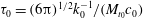
The Taylor Reynolds number, taken equal to 200 in all simulations, is based on the initial Taylor microscale, r.m.s. velocity and kinematic viscosity. The latter depends on the initial thermodynamic conditions both for air and PP11, and has to be rescaled (by a factor of the order of
 $10^{5}$
for both fluids) to match simultaneously the prescribed Mach and Reynolds number conditions.
$10^{5}$
for both fluids) to match simultaneously the prescribed Mach and Reynolds number conditions.
3 General statistics of dense gas CHIT
Direct simulations of dense gas CHIT have been carried out using a computational grid of
 $512^{3}$
cells, selected after a grid study (see appendix B).
$512^{3}$
cells, selected after a grid study (see appendix B).
The initial thermodynamic conditions used in each case are reported in table 2. Condition IC1 belongs to an isentrope that does not cross the inversion zone, yet it is characterized by an initial value of
 $\unicode[STIX]{x1D6E4}$
close to zero. At these conditions, dense gas effects are expected to be significant, although no BZT effects can appear since the entropy can only increase during the flow evolution. In the following, DNS of PP11-IC1 are carried out at various
$\unicode[STIX]{x1D6E4}$
close to zero. At these conditions, dense gas effects are expected to be significant, although no BZT effects can appear since the entropy can only increase during the flow evolution. In the following, DNS of PP11-IC1 are carried out at various
 $M_{t_{0}}$
, ranging from 0.2 to 1, and the dense gas effects are assessed by comparing the results with those of a standard diatomic gas, namely air, modelled as a PFG with
$M_{t_{0}}$
, ranging from 0.2 to 1, and the dense gas effects are assessed by comparing the results with those of a standard diatomic gas, namely air, modelled as a PFG with
 $\unicode[STIX]{x1D6FE}=1.4$
. Its viscosity is assumed to vary as a power law of the temperature and the Prandtl number is constant and equal to 0.7. In order to assess the role played by BZT effects, we have also considered a different initial state falling in the inversion zone (case PP11-IC2). The location of the initial thermodynamic states are reported in the Clapeyron diagram shown in figure 1.
$\unicode[STIX]{x1D6FE}=1.4$
. Its viscosity is assumed to vary as a power law of the temperature and the Prandtl number is constant and equal to 0.7. In order to assess the role played by BZT effects, we have also considered a different initial state falling in the inversion zone (case PP11-IC2). The location of the initial thermodynamic states are reported in the Clapeyron diagram shown in figure 1.

Figure 1. Isocontours of the reduced temperature in the Clapeyron diagram for PP11. Three iso-
 $\unicode[STIX]{x1D6E4}$
lines are also represented. The transition line (
$\unicode[STIX]{x1D6E4}$
lines are also represented. The transition line (
 $\unicode[STIX]{x1D6E4}=0$
) separates the BZT region from the dense gas region (
$\unicode[STIX]{x1D6E4}=0$
) separates the BZT region from the dense gas region (
 $\unicode[STIX]{x1D6E4}<1$
). The black dashed line denotes the critical isotherm. The white and red circles represent the initial thermodynamic conditions for cases PP11-IC1 and PP11-IC2, respectively. The latter lies in the inversion zone. White and red dash-dotted lines are used to highlight the corresponding initial isentropes.
$\unicode[STIX]{x1D6E4}<1$
). The black dashed line denotes the critical isotherm. The white and red circles represent the initial thermodynamic conditions for cases PP11-IC1 and PP11-IC2, respectively. The latter lies in the inversion zone. White and red dash-dotted lines are used to highlight the corresponding initial isentropes.
Table 2. Summary of the thermodynamic models and initial thermodynamic conditions used in the study.

In this section we discuss the time evolution of the flow statistics at various
 $M_{t_{0}}$
, focusing on condition IC1.
$M_{t_{0}}$
, focusing on condition IC1.
As shown by Lesieur (Reference Lesieur2008), decaying homogeneous isotropic turbulence exhibits a two-phase evolution. In the first phase, viscous effects are essentially negligible, worm-like structures due to sheet roll-up developing, and vortex stretching produces a large increase of enstrophy. In the second, the energy transferred to the smallest scales starts to be dissipated by viscosity. The transition from the first to the second phase is associated with the enstrophy peak.
For incompressible flows, the first phase depends essentially on the shape prescribed for the initial energy spectrum. For compressible flows, initial fluctuations of thermodynamic quantities have also to be prescribed. The initial fields being in general not a solution of the compressible Navier–Stokes equations, an acoustic transient develops. As already shown by other authors (see for example Lee et al.
Reference Lee, Lele and Moin1991) in the early stage of the first phase the flow adjusts to the initial conditions through an acoustic mechanisms on a time scale
 $\unicode[STIX]{x1D70F}_{ac}=k_{0}^{-1}/c_{0}$
, where
$\unicode[STIX]{x1D70F}_{ac}=k_{0}^{-1}/c_{0}$
, where
 $c_{0}=u_{rms_{0}}/M_{t_{0}}$
. On the other hand, the time scale corresponding to the enstrophy peak is of the same order as the initial large eddy turnover time, which is
$c_{0}=u_{rms_{0}}/M_{t_{0}}$
. On the other hand, the time scale corresponding to the enstrophy peak is of the same order as the initial large eddy turnover time, which is
 $\unicode[STIX]{x1D70F}_{0}=(6\unicode[STIX]{x03C0})^{1/2}k_{0}^{-1}/(M_{t_{0}}c_{0})$
for the assumed velocity spectrum (2.12). The ratio of the two time scales is
$\unicode[STIX]{x1D70F}_{0}=(6\unicode[STIX]{x03C0})^{1/2}k_{0}^{-1}/(M_{t_{0}}c_{0})$
for the assumed velocity spectrum (2.12). The ratio of the two time scales is
 $\unicode[STIX]{x1D70F}_{0}/\unicode[STIX]{x1D70F}_{ac}\approx M_{t_{0}}/\sqrt{6\unicode[STIX]{x03C0}}$
, showing that the acoustic transient ends long before the enstrophy peak is reached (see figure 2).
$\unicode[STIX]{x1D70F}_{0}/\unicode[STIX]{x1D70F}_{ac}\approx M_{t_{0}}/\sqrt{6\unicode[STIX]{x03C0}}$
, showing that the acoustic transient ends long before the enstrophy peak is reached (see figure 2).
Previous studies (Ristorcelli & Blaisdell Reference Ristorcelli and Blaisdell1997; Samtaney et al. Reference Samtaney, Pullin and Kosovic2001) show that, despite the final state being affected by the initial conditions, the influence of the turbulent Mach number is well recovered when using the same initialization procedure. This is mainly due to the decoupling of acoustic and vorticity modes up to relatively high turbulent Mach number conditions (Kovasznay Reference Kovasznay1953; Blaisdell et al. Reference Blaisdell, Mansour and Reynolds1993).
Figure 2 reports the time evolution of
 $K/K_{0}$
(a,b) and
$K/K_{0}$
(a,b) and
 $\unicode[STIX]{x1D6FA}/\unicode[STIX]{x1D6FA}_{0}$
(c,d), and the compensated energy spectra at a time at which the enstrophy attains approximately a peak (e,f), for various
$\unicode[STIX]{x1D6FA}/\unicode[STIX]{x1D6FA}_{0}$
(c,d), and the compensated energy spectra at a time at which the enstrophy attains approximately a peak (e,f), for various
 $M_{t_{0}}$
(a,c,e, air; b,d,f, PP11 IC1). Perfect and dense gas exhibit similar qualitative behaviours. After the initial transient, the turbulent kinetic energy decays at a rate that is weakly affected by
$M_{t_{0}}$
(a,c,e, air; b,d,f, PP11 IC1). Perfect and dense gas exhibit similar qualitative behaviours. After the initial transient, the turbulent kinetic energy decays at a rate that is weakly affected by
 $M_{t_{0}}$
, and at
$M_{t_{0}}$
, and at
 $t/\unicode[STIX]{x1D70F}_{0}=4$
approximately 75 % of the turbulent kinetic energy is dissipated. The enstrophy evolution exhibits a peak in the range
$t/\unicode[STIX]{x1D70F}_{0}=4$
approximately 75 % of the turbulent kinetic energy is dissipated. The enstrophy evolution exhibits a peak in the range
 $t/\unicode[STIX]{x1D70F}_{0}\approx 1.5{-}2$
depending on the value of
$t/\unicode[STIX]{x1D70F}_{0}\approx 1.5{-}2$
depending on the value of
 $M_{t_{0}}$
(figure 2
c,d). Due to the increased dissipation, the enstrophy peak decreases with the Mach number and tends to occur at earlier times. The figures also show that in the PFG case the decay of turbulence kinetic energy is slightly faster, and the enstrophy peak is slightly smaller than in the dense gas case for high
$M_{t_{0}}$
(figure 2
c,d). Due to the increased dissipation, the enstrophy peak decreases with the Mach number and tends to occur at earlier times. The figures also show that in the PFG case the decay of turbulence kinetic energy is slightly faster, and the enstrophy peak is slightly smaller than in the dense gas case for high
 $M_{t_{0}}$
. However, overall the behaviour of kinematic properties is little affected by the type of gas. The distribution of the computed energy spectra (figure 2
e,f) shows that, when scaled with Kolmogorov’s length scale (defined as
$M_{t_{0}}$
. However, overall the behaviour of kinematic properties is little affected by the type of gas. The distribution of the computed energy spectra (figure 2
e,f) shows that, when scaled with Kolmogorov’s length scale (defined as
 $\unicode[STIX]{x1D702}=[\langle \unicode[STIX]{x1D707}\rangle ^{3}/(\langle \unicode[STIX]{x1D700}\rangle \langle \unicode[STIX]{x1D70C}\rangle ^{2})]^{1/4}$
with
$\unicode[STIX]{x1D702}=[\langle \unicode[STIX]{x1D707}\rangle ^{3}/(\langle \unicode[STIX]{x1D700}\rangle \langle \unicode[STIX]{x1D70C}\rangle ^{2})]^{1/4}$
with
 $\unicode[STIX]{x1D700}$
the total dissipation), all data collapse well up to
$\unicode[STIX]{x1D700}$
the total dissipation), all data collapse well up to
 $k_{\mathit{max}}\unicode[STIX]{x1D702}\approx 2$
independently of
$k_{\mathit{max}}\unicode[STIX]{x1D702}\approx 2$
independently of
 $M_{t_{0}}$
. At wavenumbers close to grid cutoff (well below Kolmogorov’s one), the spectra tend to rise, likely due to small unfiltered grid-to-grid oscillations. However, their energy content is very low (below
$M_{t_{0}}$
. At wavenumbers close to grid cutoff (well below Kolmogorov’s one), the spectra tend to rise, likely due to small unfiltered grid-to-grid oscillations. However, their energy content is very low (below
 $10^{-5}$
) and does not affect the larger-scale dynamics.
$10^{-5}$
) and does not affect the larger-scale dynamics.

Figure 2. Time histories of the normalized turbulent kinetic energy (a,b), normalized enstrophy (c,d) and compensated turbulent kinetic energy spectra at
 $t/\unicode[STIX]{x1D70F}_{0}=2$
(e,f) for air (a,c,e) and PP11-IC1 (b,d,f) at various Mach numbers: ▫,
$t/\unicode[STIX]{x1D70F}_{0}=2$
(e,f) for air (a,c,e) and PP11-IC1 (b,d,f) at various Mach numbers: ▫,
 $M_{t_{0}}=0.2$
; ○,
$M_{t_{0}}=0.2$
; ○,
 $M_{t_{0}}=0.5$
; ♢,
$M_{t_{0}}=0.5$
; ♢,
 $M_{t_{0}}=0.8$
; ▵,
$M_{t_{0}}=0.8$
; ▵,
 $M_{t_{0}}=1$
.
$M_{t_{0}}=1$
.
In order to compare the time evolution of the thermodynamic properties at the various turbulent Mach numbers, the time is scaled with the acoustic time. The time histories of the r.m.s. of
 $T$
,
$T$
,
 $p$
and
$p$
and
 $\unicode[STIX]{x1D70C}$
are reported in figure 3, confirming that with the adopted time scaling, the initial acoustic transients vanish at the same time period (approximately after
$\unicode[STIX]{x1D70C}$
are reported in figure 3, confirming that with the adopted time scaling, the initial acoustic transients vanish at the same time period (approximately after
 $tc_{0}k_{0}\approx 2$
, as also found by Lee et al.
Reference Lee, Lele and Moin1991). As already observed in Sciacovelli et al. (Reference Sciacovelli, Cinnella, Content and Grasso2016) for the inviscid case, temperature and pressure fluctuations in the dense gas are much smaller than in air. Specifically, the dense gas solution significantly departs from the air one for
$tc_{0}k_{0}\approx 2$
, as also found by Lee et al.
Reference Lee, Lele and Moin1991). As already observed in Sciacovelli et al. (Reference Sciacovelli, Cinnella, Content and Grasso2016) for the inviscid case, temperature and pressure fluctuations in the dense gas are much smaller than in air. Specifically, the dense gas solution significantly departs from the air one for
 $M_{t_{0}}\geqslant 0.5$
. The observed deviations are largely due to the different molecular complexities of the two fluids since, in the ideal gas limit,
$M_{t_{0}}\geqslant 0.5$
. The observed deviations are largely due to the different molecular complexities of the two fluids since, in the ideal gas limit,
 $p_{\mathit{rms}}/p_{0}$
and
$p_{\mathit{rms}}/p_{0}$
and
 $T_{\mathit{rms}}/T_{0}$
scale approximately as
$T_{\mathit{rms}}/T_{0}$
scale approximately as
 $\unicode[STIX]{x1D6FE}M_{t_{0}}^{2}$
, and
$\unicode[STIX]{x1D6FE}M_{t_{0}}^{2}$
, and
 $\unicode[STIX]{x1D6FE}$
is approximately 40 % smaller for PP11, compared with air (Sciacovelli et al.
Reference Sciacovelli, Cinnella, Content and Grasso2016). Finally, even if the time histories of the r.m.s. of the density (not reported) are similar in both cases, in dense gases the instantaneous ratio of maximum to minimum density is much smaller. At
$\unicode[STIX]{x1D6FE}$
is approximately 40 % smaller for PP11, compared with air (Sciacovelli et al.
Reference Sciacovelli, Cinnella, Content and Grasso2016). Finally, even if the time histories of the r.m.s. of the density (not reported) are similar in both cases, in dense gases the instantaneous ratio of maximum to minimum density is much smaller. At
 $M_{t_{0}}=1$
the PFG density ratio is nearly 2.5 times greater than the dense gas. As the decay proceeds, compressibility effects decrease and the differences become smaller. This behaviour is likely due to the occurrence of compression shocklets yielding significant density variations, which are stronger in air than in a dense gas.
$M_{t_{0}}=1$
the PFG density ratio is nearly 2.5 times greater than the dense gas. As the decay proceeds, compressibility effects decrease and the differences become smaller. This behaviour is likely due to the occurrence of compression shocklets yielding significant density variations, which are stronger in air than in a dense gas.

Figure 3. Time histories of the r.m.s. temperature (a,b), r.m.s. pressure (c,d), r.m.s. density (e,f) and maximum-to-minimum density ratio (d), for air (a,c,e) and PP11-IC1 (b,d,f) at various Mach numbers: ▫,
 $M_{t_{0}}=0.2$
; ○,
$M_{t_{0}}=0.2$
; ○,
 $M_{t_{0}}=0.5$
; ♢,
$M_{t_{0}}=0.5$
; ♢,
 $M_{t_{0}}=0.8$
; ▵,
$M_{t_{0}}=0.8$
; ▵,
 $M_{t_{0}}=1$
.
$M_{t_{0}}=1$
.
The observed differences between air and PP11 are strictly related to the fluid compressibility and are better understood by looking at the time evolution of the mean and r.m.s. speed of sound, and r.m.s. dilatation (figure 4). At
 $M_{t_{0}}=0.2$
, compressibility effects are still weak in both cases and the two gases behave similarly. Departures from the standard behaviour start to become visible for
$M_{t_{0}}=0.2$
, compressibility effects are still weak in both cases and the two gases behave similarly. Departures from the standard behaviour start to become visible for
 $M_{t_{0}}=0.5$
and increase significantly at higher Mach numbers. For air,
$M_{t_{0}}=0.5$
and increase significantly at higher Mach numbers. For air,
 $\langle c\rangle$
increases with the square root of the average temperature, while for the dense gas it strongly depends on density fluctuations, leading to a scattering of the flow thermodynamic states in the
$\langle c\rangle$
increases with the square root of the average temperature, while for the dense gas it strongly depends on density fluctuations, leading to a scattering of the flow thermodynamic states in the
 $p-v$
plane (see figure 5 where we report the thermodynamic states in the Clapeyron diagram at various
$p-v$
plane (see figure 5 where we report the thermodynamic states in the Clapeyron diagram at various
 $M_{t_{0}}$
and
$M_{t_{0}}$
and
 $t/\unicode[STIX]{x1D70F}_{0}=2$
). In regions characterized by pressures higher than the initial one, the speed of sound is considerably higher than in regions where the pressure is lower, resulting in an average sound speed value higher than the initial one. At later times the scattering decreases due to turbulence decay, and
$t/\unicode[STIX]{x1D70F}_{0}=2$
). In regions characterized by pressures higher than the initial one, the speed of sound is considerably higher than in regions where the pressure is lower, resulting in an average sound speed value higher than the initial one. At later times the scattering decreases due to turbulence decay, and
 $\langle c\rangle$
decreases accordingly. The r.m.s. of the dilatation has a peak (increasing with
$\langle c\rangle$
decreases accordingly. The r.m.s. of the dilatation has a peak (increasing with
 $M_{t_{0}}$
) for the PFG case, whereas the dense gas exhibits a smoother behaviour and lower peak values. It is interesting to observe that the
$M_{t_{0}}$
) for the PFG case, whereas the dense gas exhibits a smoother behaviour and lower peak values. It is interesting to observe that the
 $\langle \unicode[STIX]{x1D6E4}\rangle$
remains below 1 throughout the decay (figure 6
a), while the
$\langle \unicode[STIX]{x1D6E4}\rangle$
remains below 1 throughout the decay (figure 6
a), while the
 $\unicode[STIX]{x1D6E4}_{\mathit{rms}}$
(figure 6
b) is of the same order as
$\unicode[STIX]{x1D6E4}_{\mathit{rms}}$
(figure 6
b) is of the same order as
 $\langle \unicode[STIX]{x1D6E4}\rangle$
due to the considerable scattering in the thermodynamic space and to the strong increase experienced by the fundamental derivative in the high pressure limit.
$\langle \unicode[STIX]{x1D6E4}\rangle$
due to the considerable scattering in the thermodynamic space and to the strong increase experienced by the fundamental derivative in the high pressure limit.

Figure 4. Time histories of normalized sound speed (a,b), r.m.s. sound speed (c,d), turbulent Mach number (e,f) and r.m.s. dilatation normalized with the initial r.m.s. vorticity (d), for air (a,c,e) and PP11-IC1 (b,d,f) at various Mach numbers: ▫,
 $M_{t_{0}}=0.2$
; ○,
$M_{t_{0}}=0.2$
; ○,
 $M_{t_{0}}=0.5$
; ♢,
$M_{t_{0}}=0.5$
; ♢,
 $M_{t_{0}}=0.8$
; ▵,
$M_{t_{0}}=0.8$
; ▵,
 $M_{t_{0}}=1$
.
$M_{t_{0}}=1$
.

Figure 5. Distribution of the thermodynamic states in the Clapeyron diagram at
 $t/\unicode[STIX]{x1D70F}_{0}=2$
for PP11-IC1 at various
$t/\unicode[STIX]{x1D70F}_{0}=2$
for PP11-IC1 at various
 $M_{t_{0}}$
: white symbols,
$M_{t_{0}}$
: white symbols,
 $M_{t_{0}}=0.5$
; red symbols,
$M_{t_{0}}=0.5$
; red symbols,
 $M_{t_{0}}=0.8$
; black symbols,
$M_{t_{0}}=0.8$
; black symbols,
 $M_{t_{0}}=1$
.
$M_{t_{0}}=1$
.

Figure 6. Time history of the average (a) and r.m.s. (b) fundamental derivative of gas dynamics for PP11-IC1 at various
 $M_{t_{0}}$
: ▫,
$M_{t_{0}}$
: ▫,
 $M_{t_{0}}=0.2$
; ○,
$M_{t_{0}}=0.2$
; ○,
 $M_{t_{0}}=0.5$
; ♢,
$M_{t_{0}}=0.5$
; ♢,
 $M_{t_{0}}=0.8$
; ▵,
$M_{t_{0}}=0.8$
; ▵,
 $M_{t_{0}}=1$
.
$M_{t_{0}}=1$
.
To understand how local compressibility effects (including eddy shocklets), influence the overall flow behaviour, in figure 7 we report the p.d.f.s of normalized dilatation. In the air case, due to the occurrence of strong compression regions (namely shocklets) the p.d.f. is characterized by a heavy left tail, whereas it becomes more and more symmetric as dense gas effects are introduced, as already observed in inviscid CHIT (Sciacovelli et al.
Reference Sciacovelli, Cinnella, Content and Grasso2016). For case PP11-IC1, the fundamental derivative is always positive and the reduction of the left tail is essentially due to the weakening of compression waves in the neighbourhood of
 $\unicode[STIX]{x1D6E4}=0$
(see (1.2)), compared to air for which
$\unicode[STIX]{x1D6E4}=0$
(see (1.2)), compared to air for which
 $\unicode[STIX]{x1D6E4}=1.2$
.
$\unicode[STIX]{x1D6E4}=1.2$
.

Figure 7. The p.d.f.s of the normalized dilatation at
 $t/\unicode[STIX]{x1D70F}_{0}=2$
for air (a) and PP11-IC1 (b) at various
$t/\unicode[STIX]{x1D70F}_{0}=2$
for air (a) and PP11-IC1 (b) at various
 $M_{t_{0}}$
: ▫,
$M_{t_{0}}$
: ▫,
 $M_{t_{0}}=0.2$
; ○,
$M_{t_{0}}=0.2$
; ○,
 $M_{t_{0}}=0.5$
; ♢,
$M_{t_{0}}=0.5$
; ♢,
 $M_{t_{0}}=0.8$
; ▵,
$M_{t_{0}}=0.8$
; ▵,
 $M_{t_{0}}=1$
.
$M_{t_{0}}=1$
.
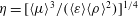
Regarding the time evolution of the viscosity and of the Eckert and Prandtl numbers, we first observe that, both for air and PP11,
 $\langle \unicode[STIX]{x1D707}\rangle$
follows the same trend as
$\langle \unicode[STIX]{x1D707}\rangle$
follows the same trend as
 $\langle c\rangle$
. Specifically
$\langle c\rangle$
. Specifically
 $\langle \unicode[STIX]{x1D707}\rangle$
varies approximately as
$\langle \unicode[STIX]{x1D707}\rangle$
varies approximately as
 $\langle T\rangle ^{0.7}$
in the PFG, while in the dense gas it is primarily driven by density variations (figure 8
a,b). As a result, viscosity grows with time in the PFG case, while it decreases (after the initial transient) in the dense gas case. For air, the maximum value reached by the viscosity during the evolution is approximately 15 % greater than the initial one (at the largest time considered in the simulations), whereas for the dense gas the peak of viscosity, reached at
$\langle T\rangle ^{0.7}$
in the PFG, while in the dense gas it is primarily driven by density variations (figure 8
a,b). As a result, viscosity grows with time in the PFG case, while it decreases (after the initial transient) in the dense gas case. For air, the maximum value reached by the viscosity during the evolution is approximately 15 % greater than the initial one (at the largest time considered in the simulations), whereas for the dense gas the peak of viscosity, reached at
 $tc_{0}k_{0}\approx 2$
, is of the order of 3 % only. The Eckert number (figure 8
c,d) is
$tc_{0}k_{0}\approx 2$
, is of the order of 3 % only. The Eckert number (figure 8
c,d) is
 $\mathit{O}(10^{-1})$
for air, whereas it is at least two orders of magnitude less for PP11, which implies that dynamical and thermal effects are loosely coupled at all
$\mathit{O}(10^{-1})$
for air, whereas it is at least two orders of magnitude less for PP11, which implies that dynamical and thermal effects are loosely coupled at all
 $M_{t_{0}}$
. Furthermore,
$M_{t_{0}}$
. Furthermore,
 $\langle Ec\rangle$
scales approximately with
$\langle Ec\rangle$
scales approximately with
 $M_{t_{0}}^{2}$
both for air and PP11. It is interesting to observe that the Prandtl number (figure 8
e), a constant for air, varies with
$M_{t_{0}}^{2}$
both for air and PP11. It is interesting to observe that the Prandtl number (figure 8
e), a constant for air, varies with
 $M_{t_{0}}$
for the dense gas, ranging approximately between 2.4 and 2.6, thus implying that energy transfer by viscous diffusion is more important than heat conduction.
$M_{t_{0}}$
for the dense gas, ranging approximately between 2.4 and 2.6, thus implying that energy transfer by viscous diffusion is more important than heat conduction.

Figure 8. Time histories of the normalized average viscosity (a,b), Eckert number (c,d) for air (a,c) and PP11-IC1 (b,d) at various Mach numbers: ▫,
 $M_{t_{0}}=0.2$
; ○,
$M_{t_{0}}=0.2$
; ○,
 $M_{t_{0}}=0.5$
; ♢,
$M_{t_{0}}=0.5$
; ♢,
 $M_{t_{0}}=0.8$
; ▵,
$M_{t_{0}}=0.8$
; ▵,
 $M_{t_{0}}=1$
. The Prandtl number (e) is reported only for PP11, being constant and equal to 0.7 for air.
$M_{t_{0}}=1$
. The Prandtl number (e) is reported only for PP11, being constant and equal to 0.7 for air.
4 Small-scale features of dense gas CHIT
4.1 Local flow topology
In turbulence, it is especially interesting to study the behaviour of critical points, i.e. points where the velocity gradient is degenerated, such as nodes, saddles, foci, etc. (Chong, Perry & Cantwell Reference Chong, Perry and Cantwell1990) and their contribution to the flow dynamics. The notion of flow topology refers to the spatial characterization of the flow field through its partitioning into simpler geometrical units, and is related to the presence of coherent turbulent structures (Wang & Peters Reference Wang and Peters2013). To elucidate the influence of dense gas effects on the statistical properties of turbulence structures, we consider the topological classification proposed by Perry & Chong (Reference Perry and Chong1987), Chong et al. (Reference Chong, Perry and Cantwell1990) and Kevlahan, Mahesh & Lee (Reference Kevlahan, Mahesh and Lee1992) in the framework of incompressible turbulence, and also employed by Pirozzoli & Grasso (Reference Pirozzoli and Grasso2004) and by Wang et al. (Reference Wang, Shi, Wang, Xiao, He and Chen2012) to analyse the small-scale behaviour of CHIT.
Let
 $\unicode[STIX]{x1D608}_{ij}\equiv \unicode[STIX]{x2202}u_{i}/\unicode[STIX]{x2202}x_{j}$
be the velocity gradient tensor, and
$\unicode[STIX]{x1D608}_{ij}\equiv \unicode[STIX]{x2202}u_{i}/\unicode[STIX]{x2202}x_{j}$
be the velocity gradient tensor, and
 $P$
,
$P$
,
 $Q$
and
$Q$
and
 $R$
be, respectively, its first, second and third invariant defined as
$R$
be, respectively, its first, second and third invariant defined as
 $$\begin{eqnarray}\left.\begin{array}{@{}c@{}}P=-\unicode[STIX]{x1D703}=-\unicode[STIX]{x1D61A}_{ii}=-(\unicode[STIX]{x1D706}_{1}+\unicode[STIX]{x1D706}_{2}+\unicode[STIX]{x1D706}_{3})\\ Q={\textstyle \frac{1}{2}}(P^{2}-\unicode[STIX]{x1D61A}_{ij}\unicode[STIX]{x1D61A}_{ij}+\unicode[STIX]{x1D61E}_{ij}\unicode[STIX]{x1D61E}_{ij})=\unicode[STIX]{x1D706}_{1}\unicode[STIX]{x1D706}_{2}+\unicode[STIX]{x1D706}_{1}\unicode[STIX]{x1D706}_{3}+\unicode[STIX]{x1D706}_{2}\unicode[STIX]{x1D706}_{3}\\ R={\textstyle \frac{1}{3}}(-P^{3}+3PQ-\unicode[STIX]{x1D61A}_{ij}\unicode[STIX]{x1D61A}_{jk}\unicode[STIX]{x1D61A}_{ki}-3\unicode[STIX]{x1D61E}_{ij}\unicode[STIX]{x1D61E}_{jk}\unicode[STIX]{x1D61A}_{ki})=-\unicode[STIX]{x1D706}_{1}\unicode[STIX]{x1D706}_{2}\unicode[STIX]{x1D706}_{3},\end{array}\right\}\end{eqnarray}$$
where
 $\unicode[STIX]{x1D61A}_{ij}=(\unicode[STIX]{x1D608}_{ij}+\unicode[STIX]{x1D608}_{ji})/2$
and
$\unicode[STIX]{x1D61A}_{ij}=(\unicode[STIX]{x1D608}_{ij}+\unicode[STIX]{x1D608}_{ji})/2$
and
 $\unicode[STIX]{x1D61E}_{ij}=(\unicode[STIX]{x1D608}_{ij}-\unicode[STIX]{x1D608}_{ji})/2$
are the strain- and rotation-rate tensor components, and
$\unicode[STIX]{x1D61E}_{ij}=(\unicode[STIX]{x1D608}_{ij}-\unicode[STIX]{x1D608}_{ji})/2$
are the strain- and rotation-rate tensor components, and
 $\unicode[STIX]{x1D706}_{i}$
the three eigenvalues of
$\unicode[STIX]{x1D706}_{i}$
the three eigenvalues of
 $\unicode[STIX]{x1D608}_{ij}$
.
$\unicode[STIX]{x1D608}_{ij}$
.
The nature of turbulent structures is classified according to the sign of the discriminant of
 $A$
:
$A$
:
 $$\begin{eqnarray}\unicode[STIX]{x1D6E5}={\textstyle \frac{27}{4}}R^{2}+\left(P^{3}-{\textstyle \frac{9}{2}}PQ\right)R+\left(Q^{3}-{\textstyle \frac{1}{4}}P^{2}Q^{2}\right).\end{eqnarray}$$
When
 $\unicode[STIX]{x1D6E5}$
is positive, the velocity gradient tensor has one real eigenvalue and two complex-conjugate ones, and focal regions are present; in contrast, when
$\unicode[STIX]{x1D6E5}$
is positive, the velocity gradient tensor has one real eigenvalue and two complex-conjugate ones, and focal regions are present; in contrast, when
 $\unicode[STIX]{x1D6E5}$
is negative, the eigenvalues of
$\unicode[STIX]{x1D6E5}$
is negative, the eigenvalues of
 $\unicode[STIX]{x1D608}_{ij}$
are all real and turbulent regions are non-focal. Moreover, in the case of incompressible turbulence (
$\unicode[STIX]{x1D608}_{ij}$
are all real and turbulent regions are non-focal. Moreover, in the case of incompressible turbulence (
 $P=0$
) flow regions are further classified according to the sign of
$P=0$
) flow regions are further classified according to the sign of
 $R$
, leading to the following families of structures:
$R$
, leading to the following families of structures:
 $$\begin{eqnarray}\left.\begin{array}{@{}ll@{}}\unicode[STIX]{x1D6E5}>0 & \left\{\begin{array}{@{}ll@{}}R<0 & \quad \text{stable focus-stretching}\\ R>0 & \quad \text{unstable focus-compressing}\end{array}\right.\\ \\ \unicode[STIX]{x1D6E5}<0 & \left\{\begin{array}{@{}ll@{}}R<0 & \quad \text{stable node-saddle-saddle}\\ R>0 & \quad \text{unstable node-saddle-saddle.}\end{array}\right.\end{array}\right\}\end{eqnarray}$$
In the case of compressible turbulence, according to the sign of
 $P$
additional topological structures can be identified, referred to as stable-focus compressing, unstable focus stretching, stable node-stable node-stable node, and unstable node-unstable node-unstable node regions (Chong et al.
Reference Chong, Perry and Cantwell1990). Focal regions are representative of vortical structures (Chong et al.
Reference Chong, Soria, Perry, Chacin, Cantwell and Na1998), whereas non-focal ones are more related to expansion/compression phenomena. In shock/turbulence interaction Kevlahan et al. (Reference Kevlahan, Mahesh and Lee1992) have analysed the evolution of turbulent structures in terms of the deviatoric strain-rate tensor (
$P$
additional topological structures can be identified, referred to as stable-focus compressing, unstable focus stretching, stable node-stable node-stable node, and unstable node-unstable node-unstable node regions (Chong et al.
Reference Chong, Perry and Cantwell1990). Focal regions are representative of vortical structures (Chong et al.
Reference Chong, Soria, Perry, Chacin, Cantwell and Na1998), whereas non-focal ones are more related to expansion/compression phenomena. In shock/turbulence interaction Kevlahan et al. (Reference Kevlahan, Mahesh and Lee1992) have analysed the evolution of turbulent structures in terms of the deviatoric strain-rate tensor (
 $\unicode[STIX]{x1D61A}_{ij}^{\ast }=\unicode[STIX]{x1D61A}_{ij}-(1/3)\unicode[STIX]{x1D61A}_{kk}\unicode[STIX]{x1D6FF}_{ij}$
) and the rotation rate tensor
$\unicode[STIX]{x1D61A}_{ij}^{\ast }=\unicode[STIX]{x1D61A}_{ij}-(1/3)\unicode[STIX]{x1D61A}_{kk}\unicode[STIX]{x1D6FF}_{ij}$
) and the rotation rate tensor
 $\unicode[STIX]{x1D61E}_{ij}$
, and have classified the flow into four structures
$\unicode[STIX]{x1D61E}_{ij}$
, and have classified the flow into four structures
 $$\begin{eqnarray}\left.\begin{array}{@{}ll@{}}W^{2}<S^{\ast 2}/2 & \text{convergence zones (essentially irrotational)}\\ S^{\ast 2}/2\leqslant W^{2}\leqslant 2S^{\ast 2} & \text{shear zones (strain dominated)}\\ W^{2}>2S^{\ast 2} & \text{eddy-dominated zones (highly rotational).}\end{array}\right\}\end{eqnarray}$$
Furthermore, they also classified turbulent structures as compressible or incompressible depending on the value of the parameter
 $\unicode[STIX]{x1D701}$
:
$\unicode[STIX]{x1D701}$
:
 $$\begin{eqnarray}\unicode[STIX]{x1D701}=\frac{\unicode[STIX]{x1D703}^{2}}{S^{\ast 2}+W^{2}};\quad \left.\begin{array}{@{}ll@{}}\unicode[STIX]{x1D701}\leqslant 0.05 & \text{incompressible structures}\\ \unicode[STIX]{x1D701}>0.05 & \text{compressible structures,}\end{array}\right\}\end{eqnarray}$$
where the threshold value of 0.05 (rather arbitrary), has been often used in the literature (Lee et al. Reference Lee, Lele and Moin1991; Kevlahan et al. Reference Kevlahan, Mahesh and Lee1992) to identify flow regions where dilatational dissipation represents more than 5 % of the total kinetic energy dissipation. All possible combinations of turbulent structures are summarized in table 3.
Table 3. Classification of turbulent regions in three-dimensional compressible flow according to Kevlahan et al. (Reference Kevlahan, Mahesh and Lee1992).

To systematically quantify the effects of local compressibility, we classify the overall flow volume into six subregions, according to the local dilatation scaled by the initial turbulent Mach number, as done in Wang et al. (Reference Wang, Shi, Wang, Xiao, He and Chen2012) and Sciacovelli et al. (Reference Sciacovelli, Cinnella, Content and Grasso2016):
-
(i) strong compressions,
 $\unicode[STIX]{x1D703}/\unicode[STIX]{x1D703}_{rms}M_{t_{0}}^{2}\in [-\infty ,-2]$
;
$\unicode[STIX]{x1D703}/\unicode[STIX]{x1D703}_{rms}M_{t_{0}}^{2}\in [-\infty ,-2]$
; -
(ii) moderate compressions,
$\unicode[STIX]{x1D703}/\unicode[STIX]{x1D703}_{rms}M_{t_{0}}^{2}\in [-2,-1]$
; -
(iii) weak compressions,
$\unicode[STIX]{x1D703}/\unicode[STIX]{x1D703}_{rms}M_{t_{0}}^{2}\in [-1,0]$
; -
(iv) weak expansions,
$\unicode[STIX]{x1D703}/\unicode[STIX]{x1D703}_{rms}M_{t_{0}}^{2}\in [0,1]$
; -
(v) moderate expansions,
$\unicode[STIX]{x1D703}/\unicode[STIX]{x1D703}_{rms}M_{t_{0}}^{2}\in [1,2]$
; -
(vi) strong expansions,
$\unicode[STIX]{x1D703}/\unicode[STIX]{x1D703}_{rms}M_{t_{0}}^{2}\in [2,\infty ]$
.
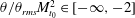
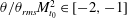
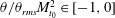
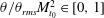
In the discussion that follows, the statistical data are plotted at time
 $t/\unicode[STIX]{x1D70F}_{0}=2$
.
$t/\unicode[STIX]{x1D70F}_{0}=2$
.
The distribution of the volume fractions occupied by the different structures conditioned on the above-defined dilatation levels is presented in figure 9 as a function of
 $M_{t_{0}}$
, for a perfect and dense gas. Up to
$M_{t_{0}}$
, for a perfect and dense gas. Up to
 $M_{t_{0}}=0.5$
, moderate and strong dilatation regions are close to zero, and the flow volume is nearly symmetrically occupied by weak expansion and compression regions. At the higher
$M_{t_{0}}=0.5$
, moderate and strong dilatation regions are close to zero, and the flow volume is nearly symmetrically occupied by weak expansion and compression regions. At the higher
 $M_{t_{0}}$
, this symmetry is rapidly lost in PFGs, due to the development of moderate and strong compressions and the progressive reduction of weak expansion regions, whereas a more symmetric behaviour is observed for PP11, as previously remarked for the p.d.f. of the local dilatation. At
$M_{t_{0}}$
, this symmetry is rapidly lost in PFGs, due to the development of moderate and strong compressions and the progressive reduction of weak expansion regions, whereas a more symmetric behaviour is observed for PP11, as previously remarked for the p.d.f. of the local dilatation. At
 $M_{t_{0}}=1$
, strong compressions occupy approximately 3.5 % of the total volume for air, while they represent about 3 % for PP11. The remaining 50 % of the flow volume is mostly occupied by weak expansions for air, while strong expansions occupy only
$M_{t_{0}}=1$
, strong compressions occupy approximately 3.5 % of the total volume for air, while they represent about 3 % for PP11. The remaining 50 % of the flow volume is mostly occupied by weak expansions for air, while strong expansions occupy only
 ${\approx}0.5\,\%$
of the total volume, in agreement with results of Wang et al. (Reference Wang, Shi, Wang, Xiao, He and Chen2012). In dense gas, strong compressions tend to be inhibited and strong expansions enhanced, leading to a nearly symmetric repartition of the volume fractions, as already observed in inviscid CHIT of BZT Van der Waals gas (Sciacovelli et al.
Reference Sciacovelli, Cinnella, Content and Grasso2016). At
${\approx}0.5\,\%$
of the total volume, in agreement with results of Wang et al. (Reference Wang, Shi, Wang, Xiao, He and Chen2012). In dense gas, strong compressions tend to be inhibited and strong expansions enhanced, leading to a nearly symmetric repartition of the volume fractions, as already observed in inviscid CHIT of BZT Van der Waals gas (Sciacovelli et al.
Reference Sciacovelli, Cinnella, Content and Grasso2016). At
 $M_{t_{0}}=1$
, weak dilatation regions occupy
$M_{t_{0}}=1$
, weak dilatation regions occupy
 ${\approx}40\,\%$
only, while moderate and strong expansion occupy, respectively, approximately 10 % and 2 % of the flow volume. The present results show that strong expansions are highly enhanced in the dense gas even when the operating conditions (IC1) do not allow BZT effects like expansion eddy shocklets. However, BZT effects contribute to further enhance expansions at the expense of compressions. Table 4 summarizes the percentage of focal and non-focal structures conditioned on the different dilatation levels as a function of the initial turbulent Mach number. The results are rather insensitive to the type of gas up to
${\approx}40\,\%$
only, while moderate and strong expansion occupy, respectively, approximately 10 % and 2 % of the flow volume. The present results show that strong expansions are highly enhanced in the dense gas even when the operating conditions (IC1) do not allow BZT effects like expansion eddy shocklets. However, BZT effects contribute to further enhance expansions at the expense of compressions. Table 4 summarizes the percentage of focal and non-focal structures conditioned on the different dilatation levels as a function of the initial turbulent Mach number. The results are rather insensitive to the type of gas up to
 $M_{t_{0}}=0.5$
. The repartition changes more and more as compressibility effects increase. At
$M_{t_{0}}=0.5$
. The repartition changes more and more as compressibility effects increase. At
 $M_{t_{0}}=1$
, focal structures occupy 63 % of the total volume for air, whereas it is 58 % for PP11-IC1 and even lower (57 %) for PP11-IC2. The largest deviations are observed in moderate and strong expansion regions. Interestingly, these regions are much more populated by non-focal structures in the dense gas than air.
$M_{t_{0}}=1$
, focal structures occupy 63 % of the total volume for air, whereas it is 58 % for PP11-IC1 and even lower (57 %) for PP11-IC2. The largest deviations are observed in moderate and strong expansion regions. Interestingly, these regions are much more populated by non-focal structures in the dense gas than air.

Figure 9. Volume fractions (%) occupied by flow regions characterized by different normalized dilatation intervals as a function of
 $M_{t_{0}}$
(
$M_{t_{0}}$
(
 $t\unicode[STIX]{x1D70F}_{0}=2$
): ——, air; – – –, PP11-IC1; — ⋅ ⋅ —, PP11-IC2; (a) strong compressions; (b) moderate compressions; (c) weak compressions; (d) weak expansions; (e) moderate expansions; (f) strong expansions.
$t\unicode[STIX]{x1D70F}_{0}=2$
): ——, air; – – –, PP11-IC1; — ⋅ ⋅ —, PP11-IC2; (a) strong compressions; (b) moderate compressions; (c) weak compressions; (d) weak expansions; (e) moderate expansions; (f) strong expansions.
Table 4. Percentage of focal/non-focal structures according to dilatation levels (at non-dimensional time
 $t/\unicode[STIX]{x1D70F}_{0}=2$
).
$t/\unicode[STIX]{x1D70F}_{0}=2$
).

For a variety of incompressible flows, including forced isotropic turbulence (Ooi et al.
Reference Ooi, Martin, Soria and Chong1999), plane mixing layers (Soria & Cantwell Reference Soria and Cantwell1994), channel flows (Blackburn, Mansour & Cantwell Reference Blackburn, Mansour and Cantwell1996) and turbulent boundary layers (Chong et al.
Reference Chong, Soria, Perry, Chacin, Cantwell and Na1998), a universal behaviour has been observed when analysing the flow topology in the
 $(Q-R)$
plane. Specifically, the joint p.d.f.
$(Q-R)$
plane. Specifically, the joint p.d.f.
 $(Q,R)$
is found to exhibit a teardrop shape. In order to analyse the influence of dense gas effects on the dynamics of CHIT, we follow the approach of Pirozzoli & Grasso (Reference Pirozzoli and Grasso2004) developed for PFG flows. We have then formulated the problem in terms of the second and third invariants of the anisotropic part of the velocity gradient tensor (
$(Q,R)$
is found to exhibit a teardrop shape. In order to analyse the influence of dense gas effects on the dynamics of CHIT, we follow the approach of Pirozzoli & Grasso (Reference Pirozzoli and Grasso2004) developed for PFG flows. We have then formulated the problem in terms of the second and third invariants of the anisotropic part of the velocity gradient tensor (
 $\unicode[STIX]{x1D608}_{ij}^{\ast }=\unicode[STIX]{x1D608}_{ij}-\unicode[STIX]{x1D703}\unicode[STIX]{x1D6FF}_{ij}/3$
):
$\unicode[STIX]{x1D608}_{ij}^{\ast }=\unicode[STIX]{x1D608}_{ij}-\unicode[STIX]{x1D703}\unicode[STIX]{x1D6FF}_{ij}/3$
):
 $$\begin{eqnarray}\displaystyle & \displaystyle Q^{\ast }=-{\textstyle \frac{1}{2}}(\unicode[STIX]{x1D61A}_{ij}^{\ast }\unicode[STIX]{x1D61A}_{ij}^{\ast }-\unicode[STIX]{x1D61E}_{ij}\unicode[STIX]{x1D61E}_{ij})=Q-{\textstyle \frac{1}{3}}P^{2} & \displaystyle\end{eqnarray}$$
 $$\begin{eqnarray}\displaystyle & \displaystyle R^{\ast }=-{\textstyle \frac{1}{3}}(\unicode[STIX]{x1D61A}_{ij}^{\ast }\unicode[STIX]{x1D61A}_{jk}^{\ast }\unicode[STIX]{x1D61A}_{ki}^{\ast }+3\unicode[STIX]{x1D61E}_{ij}\unicode[STIX]{x1D61E}_{jk}\unicode[STIX]{x1D61A}_{ki}^{\ast })=R-{\textstyle \frac{1}{3}}PQ+{\textstyle \frac{2}{27}}P^{3}, & \displaystyle\end{eqnarray}$$
where
 $\unicode[STIX]{x1D706}_{i}^{\ast }=\unicode[STIX]{x1D706}_{i}-\unicode[STIX]{x1D703}/3$
(note that, by construction,
$\unicode[STIX]{x1D706}_{i}^{\ast }=\unicode[STIX]{x1D706}_{i}-\unicode[STIX]{x1D703}/3$
(note that, by construction,
 $\unicode[STIX]{x1D6F4}\unicode[STIX]{x1D706}_{i}^{\ast }=0$
and
$\unicode[STIX]{x1D6F4}\unicode[STIX]{x1D706}_{i}^{\ast }=0$
and
 $\unicode[STIX]{x1D6E5}^{\ast }=27/4R^{\ast 2}+Q^{\ast 3}$
). A detailed analysis in the invariant plane has been carried out, the objective being twofold: (i) verify if the universal behaviour of the solenoidal component of the flow is recovered in dense gas flows, despite the peculiar thermophysical properties of these gases; (ii) investigate the influence of dense gas effects on the various flow structures.
$\unicode[STIX]{x1D6E5}^{\ast }=27/4R^{\ast 2}+Q^{\ast 3}$
). A detailed analysis in the invariant plane has been carried out, the objective being twofold: (i) verify if the universal behaviour of the solenoidal component of the flow is recovered in dense gas flows, despite the peculiar thermophysical properties of these gases; (ii) investigate the influence of dense gas effects on the various flow structures.
Even though the analysis has been conducted at various
 $M_{t_{0}}$
, in the following only results corresponding to
$M_{t_{0}}$
, in the following only results corresponding to
 $M_{t_{0}}=1$
are discussed. In figure 10 we report the
$M_{t_{0}}=1$
are discussed. In figure 10 we report the
 $\log$
of the total (a,d,g) and conditioned (b,e,h and c,f,i) joint p.d.f. of
$\log$
of the total (a,d,g) and conditioned (b,e,h and c,f,i) joint p.d.f. of
 $Q^{\ast }$
and
$Q^{\ast }$
and
 $R^{\ast }$
for air (a–c) and dense gas (PP11-IC1, d–f; PP11-IC2, g–i) for
$R^{\ast }$
for air (a–c) and dense gas (PP11-IC1, d–f; PP11-IC2, g–i) for
 $M_{t_{0}}=1$
(strong compressions, b,e,h; strong expansions, c,f,i). The joint p.d.f. is computed from the conditional averages of the data by dividing the
$M_{t_{0}}=1$
(strong compressions, b,e,h; strong expansions, c,f,i). The joint p.d.f. is computed from the conditional averages of the data by dividing the
 $(Q^{\ast },R^{\ast })$
plane into a number of equally sized partitions. For a good compromise between accuracy and statistical convergence each axis has been divided in
$(Q^{\ast },R^{\ast })$
plane into a number of equally sized partitions. For a good compromise between accuracy and statistical convergence each axis has been divided in
 $(2n)^{1/3}$
subdivisions, where
$(2n)^{1/3}$
subdivisions, where
 $n=512^{3}$
is the number of samples. As done in Chong et al. (Reference Chong, Perry and Cantwell1990) and in Pirozzoli & Grasso (Reference Pirozzoli and Grasso2004) the invariants are normalized by the average of the second invariant of the rotation-rate tensor (
$n=512^{3}$
is the number of samples. As done in Chong et al. (Reference Chong, Perry and Cantwell1990) and in Pirozzoli & Grasso (Reference Pirozzoli and Grasso2004) the invariants are normalized by the average of the second invariant of the rotation-rate tensor (
 $\langle Q_{W}\rangle =\langle \unicode[STIX]{x1D61E}_{ij}\unicode[STIX]{x1D61E}_{ij}/2\rangle$
). The thick solid line represents points where the discriminant of the anisotropic part of the deformation-rate tensor is zero (so as to discriminate between focal and non-focal regions). Independently of the type of gas, the joint p.d.f.
$\langle Q_{W}\rangle =\langle \unicode[STIX]{x1D61E}_{ij}\unicode[STIX]{x1D61E}_{ij}/2\rangle$
). The thick solid line represents points where the discriminant of the anisotropic part of the deformation-rate tensor is zero (so as to discriminate between focal and non-focal regions). Independently of the type of gas, the joint p.d.f.
 $(Q^{\ast },R^{\ast })$
exhibits a teardrop shape as in the incompressible limit (Ooi et al.
Reference Ooi, Martin, Soria and Chong1999), with a statistical preference in the second and in the fourth quadrant, where points are aligned with the right branch of the zero-discriminant curve (Cantwell Reference Cantwell1993; Martín et al.
Reference Martín, Ooi, Chong and Soria1998; Pirozzoli & Grasso Reference Pirozzoli and Grasso2004). The kinematics of critical points is thus not affected by the gas type. It is interesting to observe that conditioning on strong compressions reveals an even stronger alignment with the right branch, as in Wang et al. (Reference Wang, Shi, Wang, Xiao, He and Chen2012). However, due to the weakening/suppression of compression structures, the tail of the teardrop is shorter in the dense gas cases, especially for the BZT condition IC2. For instance the isocontour
$(Q^{\ast },R^{\ast })$
exhibits a teardrop shape as in the incompressible limit (Ooi et al.
Reference Ooi, Martin, Soria and Chong1999), with a statistical preference in the second and in the fourth quadrant, where points are aligned with the right branch of the zero-discriminant curve (Cantwell Reference Cantwell1993; Martín et al.
Reference Martín, Ooi, Chong and Soria1998; Pirozzoli & Grasso Reference Pirozzoli and Grasso2004). The kinematics of critical points is thus not affected by the gas type. It is interesting to observe that conditioning on strong compressions reveals an even stronger alignment with the right branch, as in Wang et al. (Reference Wang, Shi, Wang, Xiao, He and Chen2012). However, due to the weakening/suppression of compression structures, the tail of the teardrop is shorter in the dense gas cases, especially for the BZT condition IC2. For instance the isocontour
 $10^{-3}$
(corresponding to the bold solid line in figure 10), intersects the zero-discriminant curve at
$10^{-3}$
(corresponding to the bold solid line in figure 10), intersects the zero-discriminant curve at
 $(2.2,-3.2)$
in the case of air, against
$(2.2,-3.2)$
in the case of air, against
 $(1.93,-2.93)$
and
$(1.93,-2.93)$
and
 $(1.69,-2.69)$
for PP11-IC1 and PP11-IC2, respectively. The joint p.d.f.s conditioned on strong expansions exhibits more striking differences. For the dense gas case PP11-IC2 the p.d.f. tends to be skewed toward the left branch of the zero-discriminant curve (in particular for probability levels of
$(1.69,-2.69)$
for PP11-IC1 and PP11-IC2, respectively. The joint p.d.f.s conditioned on strong expansions exhibits more striking differences. For the dense gas case PP11-IC2 the p.d.f. tends to be skewed toward the left branch of the zero-discriminant curve (in particular for probability levels of
 $10^{-3}$
, or higher), in contrast with air and PP11-IC1 that exhibit a more symmetric shape. This suggests that different flow structures may appear in the strong expansion regions of BZT flows.
$10^{-3}$
, or higher), in contrast with air and PP11-IC1 that exhibit a more symmetric shape. This suggests that different flow structures may appear in the strong expansion regions of BZT flows.

Figure 10. Isocontours (
 $-4$
to 0, spacing equal to 1) of the
$-4$
to 0, spacing equal to 1) of the
 $\log _{10}$
of the joint p.d.f. of the scaled second and third invariants of the anisotropic part of the velocity gradient at
$\log _{10}$
of the joint p.d.f. of the scaled second and third invariants of the anisotropic part of the velocity gradient at
 $M_{t_{0}}=1$
(
$M_{t_{0}}=1$
(
 $t/\unicode[STIX]{x1D70F}_{0}=2$
) for air (a–c), PP11-IC1 (d–f) and PP11-IC2 (g–i). (a,d,g) Total joint p.d.f. (b,e,h) The p.d.f. conditioned on strong compressions (regions with
$t/\unicode[STIX]{x1D70F}_{0}=2$
) for air (a–c), PP11-IC1 (d–f) and PP11-IC2 (g–i). (a,d,g) Total joint p.d.f. (b,e,h) The p.d.f. conditioned on strong compressions (regions with
 $\unicode[STIX]{x1D703}/\unicode[STIX]{x1D703}_{rms}M_{t_{0}}^{2}\in [-\infty ,-2]$
). (c,f,i) The p.d.f. conditioned on strong expansions (regions with
$\unicode[STIX]{x1D703}/\unicode[STIX]{x1D703}_{rms}M_{t_{0}}^{2}\in [-\infty ,-2]$
). (c,f,i) The p.d.f. conditioned on strong expansions (regions with
 $\unicode[STIX]{x1D703}/\unicode[STIX]{x1D703}_{rms}M_{t_{0}}^{2}\in [2,\infty ]$
). The bold solid isoline denotes the isocontour
$\unicode[STIX]{x1D703}/\unicode[STIX]{x1D703}_{rms}M_{t_{0}}^{2}\in [2,\infty ]$
). The bold solid isoline denotes the isocontour
 $-3$
.
$-3$
.
4.2 Contribution of flow structures to dissipation
To further elucidate the influence of dense gases on focal and non-focal structures, we analyse the second invariant of the rotation-rate tensor (
 $Q_{W}=\unicode[STIX]{x1D61E}_{ij}\unicode[STIX]{x1D61E}_{ij}/2$
, a measure of the rotational energy), of the anisotropic part of the strain-rate tensor (
$Q_{W}=\unicode[STIX]{x1D61E}_{ij}\unicode[STIX]{x1D61E}_{ij}/2$
, a measure of the rotational energy), of the anisotropic part of the strain-rate tensor (
 $-Q_{S^{\ast }}=\unicode[STIX]{x1D61A}_{ij}^{\ast }\unicode[STIX]{x1D61A}_{ij}^{\ast }/2$
) and of the variance of the dilatation (
$-Q_{S^{\ast }}=\unicode[STIX]{x1D61A}_{ij}^{\ast }\unicode[STIX]{x1D61A}_{ij}^{\ast }/2$
) and of the variance of the dilatation (
 $P^{2}$
). Specifically, we consider the volume fractions occupied by focal and non-focal structures, as well as their contributions to
$P^{2}$
). Specifically, we consider the volume fractions occupied by focal and non-focal structures, as well as their contributions to
 $Q_{W}$
and
$Q_{W}$
and
 $Q_{S^{\ast }}$
, as a function of the initial turbulent Mach number.
$Q_{S^{\ast }}$
, as a function of the initial turbulent Mach number.
We recall that the total dissipation (
 $-2\overline{\unicode[STIX]{x1D707}}\langle Q_{S^{\ast }}\rangle$
) is the sum of the solenoidal (
$-2\overline{\unicode[STIX]{x1D707}}\langle Q_{S^{\ast }}\rangle$
) is the sum of the solenoidal (
 $2\overline{\unicode[STIX]{x1D707}}\langle Q_{W}\rangle$
) and dilatational (
$2\overline{\unicode[STIX]{x1D707}}\langle Q_{W}\rangle$
) and dilatational (
 $2/3\overline{\unicode[STIX]{x1D707}}\langle P^{2}\rangle$
) dissipation.
$2/3\overline{\unicode[STIX]{x1D707}}\langle P^{2}\rangle$
) dissipation.
The distributions of
 $\langle V\rangle ^{\pm }$
(where
$\langle V\rangle ^{\pm }$
(where
 $+$
and
$+$
and
 $-$
indicate conditioning on focal and non-focal structures, respectively) are reported in figure 11 as a function of
$-$
indicate conditioning on focal and non-focal structures, respectively) are reported in figure 11 as a function of
 $M_{t_{0}}$
(a,d, incompressible structures; b,e, compressed structures; c,f, expanding structures) for air and PP11-IC1. At low
$M_{t_{0}}$
(a,d, incompressible structures; b,e, compressed structures; c,f, expanding structures) for air and PP11-IC1. At low
 $M_{t_{0}}$
we observe that, in the PFG case: (i) structures of an incompressible nature occupy a larger volume fraction than compressible ones; (ii) shear-like structures are the most frequent and occupy
$M_{t_{0}}$
we observe that, in the PFG case: (i) structures of an incompressible nature occupy a larger volume fraction than compressible ones; (ii) shear-like structures are the most frequent and occupy
 ${\approx}42\,\%$
of the flow volume; and (iii) eddy and convergence zones represent
${\approx}42\,\%$
of the flow volume; and (iii) eddy and convergence zones represent
 ${\approx}19\,\%$
and
${\approx}19\,\%$
and
 ${\approx}38\,\%$
of the total flow volume, respectively. Up to
${\approx}38\,\%$
of the total flow volume, respectively. Up to
 $M_{t_{0}}=0.5$
, PP11 exhibits similar statistical volume fraction distributions. As the initial turbulent Mach number increases, the volume fraction occupied by incompressible structures is reduced significantly due to the development of compressible structures, whose volume fractions nearly triple when
$M_{t_{0}}=0.5$
, PP11 exhibits similar statistical volume fraction distributions. As the initial turbulent Mach number increases, the volume fraction occupied by incompressible structures is reduced significantly due to the development of compressible structures, whose volume fractions nearly triple when
 $M_{t_{0}}$
is varied from 0.5 to 1. As compressibility effects become significant, the volume percentage associated with the different flow structures is most affected by the working fluid. Specifically, the volume fraction of compressible structures is 58 % for PP11-IC1, whereas it is only 44 % for air, and convergence and shear compressed regions are
$M_{t_{0}}$
is varied from 0.5 to 1. As compressibility effects become significant, the volume percentage associated with the different flow structures is most affected by the working fluid. Specifically, the volume fraction of compressible structures is 58 % for PP11-IC1, whereas it is only 44 % for air, and convergence and shear compressed regions are
 ${\approx}30\,\%$
larger than in air. The choice of the initial conditions (IC1 versus IC2) has a small influence on the computed volume fractions.
${\approx}30\,\%$
larger than in air. The choice of the initial conditions (IC1 versus IC2) has a small influence on the computed volume fractions.

Figure 11. Fractional contribution of the various flow structures to
 $\langle V\rangle ^{+}$
(a–c) and
$\langle V\rangle ^{+}$
(a–c) and
 $\langle V\rangle ^{-}$
(d–f) at various
$\langle V\rangle ^{-}$
(d–f) at various
 $M_{t_{0}}$
(
$M_{t_{0}}$
(
 $t/\unicode[STIX]{x1D70F}_{0}=2$
): (a,d) incompressible structures; (b,e) compressed structures; (c,f) expanding structures; ——, air; – – –, PP11-IC1;
$t/\unicode[STIX]{x1D70F}_{0}=2$
): (a,d) incompressible structures; (b,e) compressed structures; (c,f) expanding structures; ——, air; – – –, PP11-IC1;
 $+$
, EI;
$+$
, EI;
 $\times$
, CI; ♢, SI; ▫, EC; ○, CC; ▵, SC; ▪, EE; ●, CE; ▴, SE.
$\times$
, CI; ♢, SI; ▫, EC; ○, CC; ▵, SC; ▪, EE; ●, CE; ▴, SE.
An interesting feature is that, for dense gas, expanding convergence regions (associated with strong expansion phenomena and, possibly, shocklets for the IC2 case) are almost as frequent as expanding shear zones, unlike air for which shear regions dominate. This behaviour is likely to be related to the non-convex nature of the inviscid fluxes and to the degeneracy of the characteristic fields in the proximity of the inversion zone (
 $\unicode[STIX]{x1D6E4}\approx 0$
), leading to the formation of steep expansion fronts, as discussed in greater detail in a later section.
$\unicode[STIX]{x1D6E4}\approx 0$
), leading to the formation of steep expansion fronts, as discussed in greater detail in a later section.
The isosurfaces of the strong compression regions
 $\unicode[STIX]{x1D703}/\unicode[STIX]{x1D703}_{rms}M_{t_{0}}^{2}=-3$
(a,c,e) and of the strong expansion regions
$\unicode[STIX]{x1D703}/\unicode[STIX]{x1D703}_{rms}M_{t_{0}}^{2}=-3$
(a,c,e) and of the strong expansion regions
 $\unicode[STIX]{x1D703}/\unicode[STIX]{x1D703}_{rms}M_{t_{0}}^{2}=3$
(b,d,f) are reported in figure 12 both for air (a,b) and for the dense gas cases (c–f) at
$\unicode[STIX]{x1D703}/\unicode[STIX]{x1D703}_{rms}M_{t_{0}}^{2}=3$
(b,d,f) are reported in figure 12 both for air (a,b) and for the dense gas cases (c–f) at
 $M_{t_{0}}=1$
. For air, strong compression regions are populated by random sheet-like structures of convergence-type topology over a wide range of scales, contrary to strong expansions that are characterized by sparse blob or tubular structures mainly of the eddy and shear type. The dense gas also exhibits compressed sheet-like shocklets and an increased volume percentage of expanding structures having tubular as well as sheet-like convergence topology. The continuous convergence structures steepen in the case of IC2 (figure 12
e,f), leading to expansion shocklets that are admissible since the initial thermodynamic state falls in the inversion region.
$M_{t_{0}}=1$
. For air, strong compression regions are populated by random sheet-like structures of convergence-type topology over a wide range of scales, contrary to strong expansions that are characterized by sparse blob or tubular structures mainly of the eddy and shear type. The dense gas also exhibits compressed sheet-like shocklets and an increased volume percentage of expanding structures having tubular as well as sheet-like convergence topology. The continuous convergence structures steepen in the case of IC2 (figure 12
e,f), leading to expansion shocklets that are admissible since the initial thermodynamic state falls in the inversion region.

Figure 12. Strong compressions
 $\unicode[STIX]{x1D703}/\unicode[STIX]{x1D703}_{rms}=-3$
(a,c,e) and strong expansions
$\unicode[STIX]{x1D703}/\unicode[STIX]{x1D703}_{rms}=-3$
(a,c,e) and strong expansions
 $\unicode[STIX]{x1D703}/\unicode[STIX]{x1D703}_{rms}=3$
(b,d,f) for air (a,b), PP11-IC1 (c,d) and PP11-IC2 (e,f) coloured with the local type of structure: blue, eddy; white, shear; red, convergence.
$\unicode[STIX]{x1D703}/\unicode[STIX]{x1D703}_{rms}=3$
(b,d,f) for air (a,b), PP11-IC1 (c,d) and PP11-IC2 (e,f) coloured with the local type of structure: blue, eddy; white, shear; red, convergence.
Next, we consider the fractional contributions of the different flow structures to the solenoidal, total and dilatational dissipation. For both perfect and dense gas cases, shear regions account approximately for 50 % of the solenoidal dissipation, whereas compressible regions contribute less than 20 % of the total, the contribution being slightly higher for the dense gas. In all cases, the contribution of eddy-like regions is almost negligible. Furthermore, focal and non-focal structures contribute to total dissipation by the same amount (results not reported for brevity), whereas at high
 $M_{t_{0}}$
the contribution of non-focal compressible convergence structures is significantly increased, especially in the dense gas case.
$M_{t_{0}}$
the contribution of non-focal compressible convergence structures is significantly increased, especially in the dense gas case.
The most interesting differences between the perfect and the dense gas concern the dilatational dissipation, reported in figure 13. The contribution of incompressible structures is almost the same both for air and PP11; however, the contribution of compressible structures changes significantly. We observe in particular that, for the dense gas at high
 $M_{t_{0}}$
, non-focal expanding structures play a major role, and contribute to the dilatational dissipation by an amount that is comparable to that of compressed focal structures (
$M_{t_{0}}$
, non-focal expanding structures play a major role, and contribute to the dilatational dissipation by an amount that is comparable to that of compressed focal structures (
 ${\approx}20\,\%$
versus
${\approx}20\,\%$
versus
 ${\approx}30\,\%$
). For condition IC2, for which the occurrence of expansion and compression shocklets is almost equally probable, this effect is even more accentuated (a comparison of the fractional contributions to
${\approx}30\,\%$
). For condition IC2, for which the occurrence of expansion and compression shocklets is almost equally probable, this effect is even more accentuated (a comparison of the fractional contributions to
 $\langle Q_{P}\rangle ^{\pm }$
for IC1 and IC2 is reported in figure 14). In contrast, in the PFG compressed non-focal structures (associated with the formation of eddy shocklets) contribute more significantly to dilatational dissipation than expanding ones. The amount of dilatational dissipation increases with the initial turbulent Mach number and, at
$\langle Q_{P}\rangle ^{\pm }$
for IC1 and IC2 is reported in figure 14). In contrast, in the PFG compressed non-focal structures (associated with the formation of eddy shocklets) contribute more significantly to dilatational dissipation than expanding ones. The amount of dilatational dissipation increases with the initial turbulent Mach number and, at
 $M_{t_{0}}=1$
, it represents more than 50 % of the total, whereas expanding ones contribute for less than 10 % and the dependence on
$M_{t_{0}}=1$
, it represents more than 50 % of the total, whereas expanding ones contribute for less than 10 % and the dependence on
 $M_{t_{0}}$
is weak.
$M_{t_{0}}$
is weak.

Figure 13. Fractional contribution of the various flow structures to the dilatational dissipation
 $\langle Q_{P}\rangle ^{+}$
(a–c) and
$\langle Q_{P}\rangle ^{+}$
(a–c) and
 $\langle Q_{P}\rangle ^{-}$
(d–f) at various
$\langle Q_{P}\rangle ^{-}$
(d–f) at various
 $M_{t_{0}}$
(
$M_{t_{0}}$
(
 $t/\unicode[STIX]{x1D70F}_{0}=2$
): (a,d) incompressible structures; (b,e) compressed structures; (c,f) expanding structures; ——, air; – – –, PP11-IC1;
$t/\unicode[STIX]{x1D70F}_{0}=2$
): (a,d) incompressible structures; (b,e) compressed structures; (c,f) expanding structures; ——, air; – – –, PP11-IC1;
 $+$
, EI;
$+$
, EI;
 $\times$
, CI; ♢, SI; ▫, EC; ○, CC; ▵, SC; ▪, EE; ●, CE; ▴, SE.
$\times$
, CI; ♢, SI; ▫, EC; ○, CC; ▵, SC; ▪, EE; ●, CE; ▴, SE.

Figure 14. Influence of the initial thermodynamic state on the fractional contribution of the various flow structures to the dilatational dissipation
 $\langle Q_{P}\rangle ^{+}$
(a–c) and
$\langle Q_{P}\rangle ^{+}$
(a–c) and
 $\langle Q_{P}\rangle ^{-}$
(d–f) at various
$\langle Q_{P}\rangle ^{-}$
(d–f) at various
 $M_{t_{0}}$
(
$M_{t_{0}}$
(
 $t/\unicode[STIX]{x1D70F}_{0}=2$
): (a,d) incompressible structures; (b,e) compressed structures; (c,f) expanding structures; – – –, PP11-IC1; — ⋅ ⋅ —, PP11-IC2;
$t/\unicode[STIX]{x1D70F}_{0}=2$
): (a,d) incompressible structures; (b,e) compressed structures; (c,f) expanding structures; – – –, PP11-IC1; — ⋅ ⋅ —, PP11-IC2;
 $+$
, EI;
$+$
, EI;
 $\times$
, CI; ♢, SI; ▫, EC; ○, CC; ▵, SC; ▪, EE; ●, CE; ▴, SE.
$\times$
, CI; ♢, SI; ▫, EC; ○, CC; ▵, SC; ▪, EE; ●, CE; ▴, SE.
To further investigate the correlation between the various flow structures and the occurrence of strong compression/expansion phenomena, in figure 15 we report the volume fractions of the different flow structures conditioned with respect to strong compression (
 $\unicode[STIX]{x1D703}/\unicode[STIX]{x1D703}_{rms}M_{t_{0}}^{2}<-2$
) and strong expansion zones (
$\unicode[STIX]{x1D703}/\unicode[STIX]{x1D703}_{rms}M_{t_{0}}^{2}<-2$
) and strong expansion zones (
 $\unicode[STIX]{x1D703}/\unicode[STIX]{x1D703}_{rms}M_{t_{0}}^{2}>2$
). The former are populated by similar structures both in the perfect and dense gas, with convergence compressed zones representing more than 80 % of the total volume and eddy zones being negligible. In the case of dense gas, convergence and shear zones represent, respectively, 75–80 % (depending on the initial thermodynamic state) and 15–20 % (eddy-like being negligible) of the volume occupied by expanding structures, whereas in air the different flow structures are nearly equally probable (45 % shear, 30 % convergence and 25 % eddy-like).
$\unicode[STIX]{x1D703}/\unicode[STIX]{x1D703}_{rms}M_{t_{0}}^{2}>2$
). The former are populated by similar structures both in the perfect and dense gas, with convergence compressed zones representing more than 80 % of the total volume and eddy zones being negligible. In the case of dense gas, convergence and shear zones represent, respectively, 75–80 % (depending on the initial thermodynamic state) and 15–20 % (eddy-like being negligible) of the volume occupied by expanding structures, whereas in air the different flow structures are nearly equally probable (45 % shear, 30 % convergence and 25 % eddy-like).

Figure 15. Volume fractions of the various flow structures conditioned with respect to strong compression regions (a) and strong expansion regions (b) at various
 $M_{t_{0}}$
(
$M_{t_{0}}$
(
 $t/\unicode[STIX]{x1D70F}_{0}=2$
): ——, air; – – –, PP11-IC1; — ⋅ ⋅ —, PP11-IC2; ▫, EC; ○, CC; ▵, SC; ▪, EE; ●, CE; ▴, SE.
$t/\unicode[STIX]{x1D70F}_{0}=2$
): ——, air; – – –, PP11-IC1; — ⋅ ⋅ —, PP11-IC2; ▫, EC; ○, CC; ▵, SC; ▪, EE; ●, CE; ▴, SE.
The preceding analysis supports the conclusion that, in dense gases, strong expansion regions are populated by a significant number of convergence structures that contribute considerably to the dilatational dissipation. In this sense, these regions tend to exhibit a behaviour similar to compression regions. This phenomenon is observed not only for BZT flow conditions (IC2) but also for non-BZT conditions characterized by
 $\unicode[STIX]{x1D6E4}\approx 0$
(IC1), although to a lesser extent. A possible mechanism enhancing convergence structure is the formation of steep expansion fronts (for IC1) or possibly expansion shocklets (for IC2).
$\unicode[STIX]{x1D6E4}\approx 0$
(IC1), although to a lesser extent. A possible mechanism enhancing convergence structure is the formation of steep expansion fronts (for IC1) or possibly expansion shocklets (for IC2).
4.3 Enstrophy generation mechanisms
In the preceding section we highlighted that dense gas effects modify the contribution of the various flow structures to the dilatational dissipation, whereas the rotational energy (related to enstrophy) is less affected. On the other hand, in compressible flows enstrophy is contributed by shocks in addition to shear layers and vortical motions. It is then interesting to analyse how dense gas effects modify sources of enstrophy generation. We recall that enstrophy is governed by the following transport equation (Erlebacher & Sarkar Reference Erlebacher and Sarkar1993):
 $$\begin{eqnarray}\frac{\text{D}}{\text{D}t}\left(\frac{\unicode[STIX]{x1D714}^{2}}{2}\right)=\unicode[STIX]{x1D714}_{i}V_{i}^{T}+\unicode[STIX]{x1D714}_{i}\unicode[STIX]{x1D716}_{ijk}\frac{1}{\unicode[STIX]{x1D70C}^{2}}\frac{\unicode[STIX]{x2202}\unicode[STIX]{x1D70C}}{\unicode[STIX]{x2202}x_{j}}\frac{\unicode[STIX]{x2202}p}{\unicode[STIX]{x2202}x_{k}}+\unicode[STIX]{x1D714}_{i}\unicode[STIX]{x1D716}_{ijk}\frac{\unicode[STIX]{x2202}}{\unicode[STIX]{x2202}x_{j}}\left(\frac{1}{\unicode[STIX]{x1D70C}}\frac{\unicode[STIX]{x2202}\unicode[STIX]{x1D70E}_{mk}}{\unicode[STIX]{x2202}x_{m}}\right),\end{eqnarray}$$
where
 $\unicode[STIX]{x1D714}^{2}/2=-4Q_{W}=\unicode[STIX]{x1D714}_{i}\unicode[STIX]{x1D714}_{i}/2$
is the enstrophy density,
$\unicode[STIX]{x1D714}^{2}/2=-4Q_{W}=\unicode[STIX]{x1D714}_{i}\unicode[STIX]{x1D714}_{i}/2$
is the enstrophy density,
 $\unicode[STIX]{x1D714}_{i}$
is the vorticity vector and
$\unicode[STIX]{x1D714}_{i}$
is the vorticity vector and
 $\unicode[STIX]{x1D716}_{ijk}$
is the Levi-Civita symbol. The three terms on the right-hand side represent, respectively, enstrophy generation due to vortex stretching, the baroclinic term and the viscous diffusion. The vortex stretching vector
$\unicode[STIX]{x1D716}_{ijk}$
is the Levi-Civita symbol. The three terms on the right-hand side represent, respectively, enstrophy generation due to vortex stretching, the baroclinic term and the viscous diffusion. The vortex stretching vector
 $V_{i}^{T}$
is the sum of two contributions due to the deviatoric strain rate (
$V_{i}^{T}$
is the sum of two contributions due to the deviatoric strain rate (
 $V_{i}^{S}=\unicode[STIX]{x1D714}_{j}\unicode[STIX]{x1D61A}_{ij}^{\ast }$
) and to dilatation (
$V_{i}^{S}=\unicode[STIX]{x1D714}_{j}\unicode[STIX]{x1D61A}_{ij}^{\ast }$
) and to dilatation (
 $V_{i}^{D}=-2/3\unicode[STIX]{x1D703}\unicode[STIX]{x1D714}_{i}$
).
$V_{i}^{D}=-2/3\unicode[STIX]{x1D703}\unicode[STIX]{x1D714}_{i}$
).
Integration of (4.8) over the entire volume yields
 $$\begin{eqnarray}\frac{\text{D}\langle \unicode[STIX]{x1D714}^{2}/2\rangle }{\text{D}t}=\langle \unicode[STIX]{x1D714}_{i}V_{i}^{S}\rangle +\langle \unicode[STIX]{x1D714}_{i}V_{i}^{D}\rangle +\left\langle \unicode[STIX]{x1D714}_{i}\unicode[STIX]{x1D716}_{ijk}\frac{1}{\unicode[STIX]{x1D70C}^{2}}\frac{\unicode[STIX]{x2202}\unicode[STIX]{x1D70C}}{\unicode[STIX]{x2202}x_{j}}\frac{\unicode[STIX]{x2202}p}{\unicode[STIX]{x2202}x_{k}}\right\rangle +\left\langle \unicode[STIX]{x1D714}_{i}\unicode[STIX]{x1D716}_{ijk}\frac{\unicode[STIX]{x2202}}{\unicode[STIX]{x2202}x_{j}}\left(\frac{1}{\unicode[STIX]{x1D70C}}\frac{\unicode[STIX]{x2202}\unicode[STIX]{x1D70E}_{mk}}{\unicode[STIX]{x2202}x_{m}}\right)\right\rangle .\end{eqnarray}$$
Kida & Orszag (Reference Kida and Orszag1989), Pirozzoli & Grasso (Reference Pirozzoli and Grasso2004) and Wang et al. (Reference Wang, Shi, Wang, Xiao, He and Chen2012) showed that the baroclinic effects are negative and rather negligible, while the viscous dissipation acts as a sink.
We focus our analysis on the action of the strain rate
 $\langle \unicode[STIX]{x1D714}_{i}V_{i}^{S}\rangle$
and dilatation
$\langle \unicode[STIX]{x1D714}_{i}V_{i}^{S}\rangle$
and dilatation
 $\langle \unicode[STIX]{x1D714}_{i}V_{i}^{D}\rangle$
terms. To relate enstrophy generation with the occurrence of shocklets, as in Wang et al. (Reference Wang, Shi, Wang, Xiao, He and Chen2012), we project the vorticity and the vortex stretching vectors (both the one associated with the deviatoric strain rate and the dilatation rate) in the normal and tangential directions relative to the local density isosurfaces, i.e. the direction aligned with the density gradient
$\langle \unicode[STIX]{x1D714}_{i}V_{i}^{D}\rangle$
terms. To relate enstrophy generation with the occurrence of shocklets, as in Wang et al. (Reference Wang, Shi, Wang, Xiao, He and Chen2012), we project the vorticity and the vortex stretching vectors (both the one associated with the deviatoric strain rate and the dilatation rate) in the normal and tangential directions relative to the local density isosurfaces, i.e. the direction aligned with the density gradient
 $\boldsymbol{n}=\text{grad}(\unicode[STIX]{x1D70C})/\Vert \text{grad}(\unicode[STIX]{x1D70C})\Vert$
and a direction
$\boldsymbol{n}=\text{grad}(\unicode[STIX]{x1D70C})/\Vert \text{grad}(\unicode[STIX]{x1D70C})\Vert$
and a direction
 $\boldsymbol{t}$
orthogonal to
$\boldsymbol{t}$
orthogonal to
 $\boldsymbol{n}$
.
$\boldsymbol{n}$
.

Figure 16. Distribution of the averages of the vortex stretching vector
 $\unicode[STIX]{x1D714}_{i}V_{i}^{T}$
(a,d),
$\unicode[STIX]{x1D714}_{i}V_{i}^{T}$
(a,d),
 $\unicode[STIX]{x1D714}_{i}V_{i}^{D}$
(b,e) and
$\unicode[STIX]{x1D714}_{i}V_{i}^{D}$
(b,e) and
 $\unicode[STIX]{x1D714}_{i}V_{i}^{S}$
(c,f) normalized by
$\unicode[STIX]{x1D714}_{i}V_{i}^{S}$
(c,f) normalized by
 $\langle \unicode[STIX]{x1D714}_{i}\unicode[STIX]{x1D714}_{j}\unicode[STIX]{x1D61A}_{ij}^{\ast }\rangle$
and conditioned on the dilatation for air (a–c) and PP11-IC1 (d–f) at
$\langle \unicode[STIX]{x1D714}_{i}\unicode[STIX]{x1D714}_{j}\unicode[STIX]{x1D61A}_{ij}^{\ast }\rangle$
and conditioned on the dilatation for air (a–c) and PP11-IC1 (d–f) at
 $M_{t_{0}}=1$
(
$M_{t_{0}}=1$
(
 $t/\unicode[STIX]{x1D70F}_{0}=2$
). In each panel the contributions to enstrophy generation in the direction parallel (-–○-–
$t/\unicode[STIX]{x1D70F}_{0}=2$
). In each panel the contributions to enstrophy generation in the direction parallel (-–○-–
 $r=n$
) and tangential (-- --▵-- --
$r=n$
) and tangential (-- --▵-- --
 $r=t$
) to the density gradient and the total contribution (--.--▿--.--) are reported.
$r=t$
) to the density gradient and the total contribution (--.--▿--.--) are reported.
In figure 16 we report the volume average of the rate of total enstrophy generation
 $\langle \unicode[STIX]{x1D714}_{i}V_{i}^{T}\rangle$
(a,d), the rate of dilatational enstrophy generation
$\langle \unicode[STIX]{x1D714}_{i}V_{i}^{T}\rangle$
(a,d), the rate of dilatational enstrophy generation
 $\langle \unicode[STIX]{x1D714}_{i}V_{i}^{D}\rangle$
(b,e) and the deviatoric strain-rate enstrophy generation
$\langle \unicode[STIX]{x1D714}_{i}V_{i}^{D}\rangle$
(b,e) and the deviatoric strain-rate enstrophy generation
 $\langle \unicode[STIX]{x1D714}_{i}V_{i}^{S}\rangle$
(c,f) conditioned on dilatation, both for air (a–c) and dense gas (d–f). The vorticity vector having a tendency to be orthogonal to the density gradient, the main contribution to enstrophy generation is in the tangential direction. Enstrophy is produced due to vortex stretching across eddy shocklets (compressed structures). Expanding PFG structures destroy enstrophy and both
$\langle \unicode[STIX]{x1D714}_{i}V_{i}^{S}\rangle$
(c,f) conditioned on dilatation, both for air (a–c) and dense gas (d–f). The vorticity vector having a tendency to be orthogonal to the density gradient, the main contribution to enstrophy generation is in the tangential direction. Enstrophy is produced due to vortex stretching across eddy shocklets (compressed structures). Expanding PFG structures destroy enstrophy and both
 $\langle \unicode[STIX]{x1D714}_{i}V_{i}^{S}\rangle$
and
$\langle \unicode[STIX]{x1D714}_{i}V_{i}^{S}\rangle$
and
 $\langle \unicode[STIX]{x1D714}_{i}V_{i}^{D}\rangle$
increase rapidly in magnitude with
$\langle \unicode[STIX]{x1D714}_{i}V_{i}^{D}\rangle$
increase rapidly in magnitude with
 $\unicode[STIX]{x1D703}$
. On the contrary, dense gases have a tendency to strongly inhibit enstrophy destruction across moderate and strong expansions. Furthermore, dilatational enstrophy generation is of comparable order both in the directions normal and tangential to the expanding structures. The attenuation of enstrophy destruction in expansion regions is likely due to two competing mechanisms: expansion processes associated with thermodynamic states having
$\unicode[STIX]{x1D703}$
. On the contrary, dense gases have a tendency to strongly inhibit enstrophy destruction across moderate and strong expansions. Furthermore, dilatational enstrophy generation is of comparable order both in the directions normal and tangential to the expanding structures. The attenuation of enstrophy destruction in expansion regions is likely due to two competing mechanisms: expansion processes associated with thermodynamic states having
 $\unicode[STIX]{x1D6E4}=O(1)$
that contribute to enstrophy destruction as in PFGs, and (strong) expansions associated with thermodynamic states having
$\unicode[STIX]{x1D6E4}=O(1)$
that contribute to enstrophy destruction as in PFGs, and (strong) expansions associated with thermodynamic states having
 $\unicode[STIX]{x1D6E4}$
close to or less than zero that have a tendency to behave similar to compressions (thus producing enstrophy and counteracting its destruction).
$\unicode[STIX]{x1D6E4}$
close to or less than zero that have a tendency to behave similar to compressions (thus producing enstrophy and counteracting its destruction).
To further elucidate into the enstrophy generation mechanism and its relation with the flow topology, we have also analysed the contribution due to vortex stretching in the eigendirections of the deviatoric strain rate. We recall that in incompressible flows (Ashurst et al.
Reference Ashurst, Kerstein, Kerr and Gibson1987; Cantwell Reference Cantwell1993), vorticity has a tendency to align with the eigendirection associated with the intermediate eigenvalue of the strain rate, which is found to be positive in the average (i.e. more often positive than negative). For compressible flows, we consider the deviatoric strain rate
 $\unicode[STIX]{x1D61A}_{ij}^{\ast }$
and project the vortex stretching vector in the eigendirections
$\unicode[STIX]{x1D61A}_{ij}^{\ast }$
and project the vortex stretching vector in the eigendirections
 $\unicode[STIX]{x1D726}_{k}$
associated with the eigenvalues
$\unicode[STIX]{x1D726}_{k}$
associated with the eigenvalues
 $\unicode[STIX]{x1D706}_{k}^{\ast }$
of
$\unicode[STIX]{x1D706}_{k}^{\ast }$
of
 $\unicode[STIX]{x1D61A}_{ij}^{\ast }$
. The vortex stretching term then reduces to
$\unicode[STIX]{x1D61A}_{ij}^{\ast }$
. The vortex stretching term then reduces to
 $$\begin{eqnarray}\unicode[STIX]{x1D714}_{i}\unicode[STIX]{x1D714}_{j}\unicode[STIX]{x1D61A}_{ij}^{\ast }=\unicode[STIX]{x1D714}^{2}\mathop{\sum }_{k}\unicode[STIX]{x1D706}_{k}^{\ast }\cos ^{2}\unicode[STIX]{x1D719}_{k},\end{eqnarray}$$
where
 $\unicode[STIX]{x1D719}_{k}=\cos ^{-1}(\unicode[STIX]{x1D74E}\boldsymbol{\cdot }\unicode[STIX]{x1D726}_{k}/\Vert \unicode[STIX]{x1D74E}\Vert \,\Vert \unicode[STIX]{x1D726}_{k}\Vert )$
is the angle between the vorticity vector and the
$\unicode[STIX]{x1D719}_{k}=\cos ^{-1}(\unicode[STIX]{x1D74E}\boldsymbol{\cdot }\unicode[STIX]{x1D726}_{k}/\Vert \unicode[STIX]{x1D74E}\Vert \,\Vert \unicode[STIX]{x1D726}_{k}\Vert )$
is the angle between the vorticity vector and the
 $k$
th eigendirection.
$k$
th eigendirection.

Figure 17. Conditional averages of squares of cosines of angles between the density gradient direction
 $\boldsymbol{n}$
and the strain-rate eigenvectors
$\boldsymbol{n}$
and the strain-rate eigenvectors
 $\unicode[STIX]{x1D726}_{k}$
for air (a), PP11-IC1 (b) and PP11-IC2 (c) at
$\unicode[STIX]{x1D726}_{k}$
for air (a), PP11-IC1 (b) and PP11-IC2 (c) at
 $M_{t_{0}}=1$
(
$M_{t_{0}}=1$
(
 $t/\unicode[STIX]{x1D70F}_{0}=2$
):
-–○-–,
$t/\unicode[STIX]{x1D70F}_{0}=2$
):
-–○-–,
 $k=1$
;
-- --▵-- --,
$k=1$
;
-- --▵-- --,
 $k=2$
;
--.--▿--.--,
$k=2$
;
--.--▿--.--,
 $k=3$
.
$k=3$
.
The p.d.f.s and the conditional p.d.f.s of the eigenvalue ratios
 $\unicode[STIX]{x1D706}_{2}^{\ast }/\unicode[STIX]{x1D706}_{1}^{\ast }$
and
$\unicode[STIX]{x1D706}_{2}^{\ast }/\unicode[STIX]{x1D706}_{1}^{\ast }$
and
 $\unicode[STIX]{x1D706}_{2}^{\ast }/\unicode[STIX]{x1D706}_{3}^{\ast }$
of the deviatoric strain rate for air and PP11 (not reported for brevity), as well as the conditional p.d.f.s of the normalized eigenvalues of the strain-rate tensor
$\unicode[STIX]{x1D706}_{2}^{\ast }/\unicode[STIX]{x1D706}_{3}^{\ast }$
of the deviatoric strain rate for air and PP11 (not reported for brevity), as well as the conditional p.d.f.s of the normalized eigenvalues of the strain-rate tensor
 $\unicode[STIX]{x1D6FD}_{k}=\unicode[STIX]{x1D706}_{k}/\sqrt{\sum _{i}\unicode[STIX]{x1D706}_{i}^{2}}$
, follow the classical behaviour observed both in incompressible and compressible turbulence (Ashurst et al.
Reference Ashurst, Kerstein, Kerr and Gibson1987; Erlebacher & Sarkar Reference Erlebacher and Sarkar1993; Pirozzoli & Grasso Reference Pirozzoli and Grasso2004; Lee, Girimaji & Kerimo Reference Lee, Girimaji and Kerimo2009; Wang et al.
Reference Wang, Shi, Wang, Xiao, He and Chen2012). Specifically, the most probable values of
$\unicode[STIX]{x1D6FD}_{k}=\unicode[STIX]{x1D706}_{k}/\sqrt{\sum _{i}\unicode[STIX]{x1D706}_{i}^{2}}$
, follow the classical behaviour observed both in incompressible and compressible turbulence (Ashurst et al.
Reference Ashurst, Kerstein, Kerr and Gibson1987; Erlebacher & Sarkar Reference Erlebacher and Sarkar1993; Pirozzoli & Grasso Reference Pirozzoli and Grasso2004; Lee, Girimaji & Kerimo Reference Lee, Girimaji and Kerimo2009; Wang et al.
Reference Wang, Shi, Wang, Xiao, He and Chen2012). Specifically, the most probable values of
 $\unicode[STIX]{x1D706}_{k}^{\ast }$
are approximately in the ratio
$\unicode[STIX]{x1D706}_{k}^{\ast }$
are approximately in the ratio
 $[-4:1:3]$
. Furthermore, as compression increases, the p.d.f. of
$[-4:1:3]$
. Furthermore, as compression increases, the p.d.f. of
 $\unicode[STIX]{x1D6FD}_{1}$
peaks at lower values,
$\unicode[STIX]{x1D6FD}_{1}$
peaks at lower values,
 $\unicode[STIX]{x1D6FD}_{2}$
and
$\unicode[STIX]{x1D6FD}_{2}$
and
 $\unicode[STIX]{x1D6FD}_{3}$
become much smaller than
$\unicode[STIX]{x1D6FD}_{3}$
become much smaller than
 $\unicode[STIX]{x1D6FD}_{1}$
and the eigenvalues are approximately in the ratio
$\unicode[STIX]{x1D6FD}_{1}$
and the eigenvalues are approximately in the ratio
 $[-1:0:0]$
. In strongly expanding regions the p.d.f. of
$[-1:0:0]$
. In strongly expanding regions the p.d.f. of
 $\unicode[STIX]{x1D6FD}_{3}$
peaks at approximately 1 and the eigenvalues are in the ratio
$\unicode[STIX]{x1D6FD}_{3}$
peaks at approximately 1 and the eigenvalues are in the ratio
 $[0:0:1]$
. Hence compression is dominant in the first eigendirection, while expansion is dominant in the third one.
$[0:0:1]$
. Hence compression is dominant in the first eigendirection, while expansion is dominant in the third one.
Reported in figure 17 are the conditional averages of the squared cosines of the angles between the density gradient direction and the principal strain ones (
 $\unicode[STIX]{x1D713}_{k}=\cos ^{-1}(\boldsymbol{n}\boldsymbol{\cdot }\unicode[STIX]{x1D726}_{k})/(\Vert \unicode[STIX]{x1D726}_{k}\Vert )$
) for air (a), PP11-IC1 (b) and PP11-IC2 (c) at
$\unicode[STIX]{x1D713}_{k}=\cos ^{-1}(\boldsymbol{n}\boldsymbol{\cdot }\unicode[STIX]{x1D726}_{k})/(\Vert \unicode[STIX]{x1D726}_{k}\Vert )$
) for air (a), PP11-IC1 (b) and PP11-IC2 (c) at
 $M_{t_{0}}=1$
(
$M_{t_{0}}=1$
(
 $t/\unicode[STIX]{x1D70F}_{0}=2$
). In strong compressions, the eigendirection associated with the most negative eigenvalue of
$t/\unicode[STIX]{x1D70F}_{0}=2$
). In strong compressions, the eigendirection associated with the most negative eigenvalue of
 $\unicode[STIX]{x1D61A}_{ij}$
has a tendency to align with the density gradient (i.e. it tends to be perpendicular to shocklets) both for the perfect and the dense gas. In expansion regions, the first eigenvector is nearly orthogonal to the density gradient, while the third strain-rate eigendirection has a tendency to somewhat align with the density gradient. This tendency is strongly marked in dense gas, supporting the possibility of the occurrence of steep expansion fronts for condition IC1 and eventually expansion shocklets for IC2.
$\unicode[STIX]{x1D61A}_{ij}$
has a tendency to align with the density gradient (i.e. it tends to be perpendicular to shocklets) both for the perfect and the dense gas. In expansion regions, the first eigenvector is nearly orthogonal to the density gradient, while the third strain-rate eigendirection has a tendency to somewhat align with the density gradient. This tendency is strongly marked in dense gas, supporting the possibility of the occurrence of steep expansion fronts for condition IC1 and eventually expansion shocklets for IC2.
From (4.10) we observe that the amount of enstrophy production/destruction depends on the alignment between vorticity and the deviatoric strain-rate eigendirections, and on the sign and magnitude of the associated eigenvalues. An inspection of the p.d.f.s and the conditional p.d.f.s of the angles between vorticity and
 $\unicode[STIX]{x1D726}_{k}$
(not reported), shows that the vorticity is preferentially parallel or antiparallel to the intermediate eigenvector, and has a tendency to be orthogonal to the first eigendirection. The angle between vorticity and the eigendirection associated with the most positive eigenvector has a tendency to be more uniformly distributed as expansion strengthens (i.e. any angle between vorticity and
$\unicode[STIX]{x1D726}_{k}$
(not reported), shows that the vorticity is preferentially parallel or antiparallel to the intermediate eigenvector, and has a tendency to be orthogonal to the first eigendirection. The angle between vorticity and the eigendirection associated with the most positive eigenvector has a tendency to be more uniformly distributed as expansion strengthens (i.e. any angle between vorticity and
 $\unicode[STIX]{x1D726}_{3}$
is equally probable). This behaviour, which is in agreement with the results of Wang et al. (Reference Wang, Shi, Wang, Xiao, He and Chen2012), does not depend on the type of gas and is rather similar to that observed in incompressible flows (Erlebacher & Sarkar Reference Erlebacher and Sarkar1993).
$\unicode[STIX]{x1D726}_{3}$
is equally probable). This behaviour, which is in agreement with the results of Wang et al. (Reference Wang, Shi, Wang, Xiao, He and Chen2012), does not depend on the type of gas and is rather similar to that observed in incompressible flows (Erlebacher & Sarkar Reference Erlebacher and Sarkar1993).
The conditional averages of enstrophy production by vortex stretching in the principal strain-rate directions is reported in figure 18 for air (a), PP11-IC1 (b) and PP11-IC2 (c). For air, the main contributions to enstrophy production in strong compression are associated with the second and third eigenvectors, whereas in regions where the gas undergoes strong expansions the small positive contribution in the direction associated with the most positive eigenvalue (
 $\unicode[STIX]{x1D706}_{3}^{\ast }$
) is overwhelmed by the negative contributions in the other directions, as also found by Wang et al. (Reference Wang, Shi, Wang, Xiao, He and Chen2012). For dense gas, a similar behaviour is observed in compression regions. However, in expansion zones the large negative contributions in the
$\unicode[STIX]{x1D706}_{3}^{\ast }$
) is overwhelmed by the negative contributions in the other directions, as also found by Wang et al. (Reference Wang, Shi, Wang, Xiao, He and Chen2012). For dense gas, a similar behaviour is observed in compression regions. However, in expansion zones the large negative contributions in the
 $\unicode[STIX]{x1D726}_{1}$
and
$\unicode[STIX]{x1D726}_{1}$
and
 $\unicode[STIX]{x1D726}_{2}$
eigendirections are reduced by one order of magnitude, yielding striking differences with the perfect gas case. This can be interpreted by examining the vorticity distribution whose conditional average is reported in figure 19 as a function of dilatation. In general, dense gas effects reduce vorticity both in compression and expansion zones. In strong compressions, perfect and dense gases generate a comparable average vorticity. On the contrary, in strong expansions dense gas exhibits a stronger decrease in vorticity. The p.d.f. of vorticity magnitude conditioned on dilatation is reported in figure 20, which shows indeed that high vorticity magnitudes are somewhat less probable in dense gas (the effect being stronger for case PP11-IC2) than in PFG.
$\unicode[STIX]{x1D726}_{2}$
eigendirections are reduced by one order of magnitude, yielding striking differences with the perfect gas case. This can be interpreted by examining the vorticity distribution whose conditional average is reported in figure 19 as a function of dilatation. In general, dense gas effects reduce vorticity both in compression and expansion zones. In strong compressions, perfect and dense gases generate a comparable average vorticity. On the contrary, in strong expansions dense gas exhibits a stronger decrease in vorticity. The p.d.f. of vorticity magnitude conditioned on dilatation is reported in figure 20, which shows indeed that high vorticity magnitudes are somewhat less probable in dense gas (the effect being stronger for case PP11-IC2) than in PFG.

Figure 18. Conditional averages of enstrophy production associated with the three strain-rate eigenvectors at
 $M_{t_{0}}=1$
(
$M_{t_{0}}=1$
(
 $t/\unicode[STIX]{x1D70F}_{0}=2$
) normalized by
$t/\unicode[STIX]{x1D70F}_{0}=2$
) normalized by
 $\langle \unicode[STIX]{x1D714}_{i}\unicode[STIX]{x1D714}_{j}\unicode[STIX]{x1D61A}_{ij}^{\ast }\rangle$
:
-–○-–,
$\langle \unicode[STIX]{x1D714}_{i}\unicode[STIX]{x1D714}_{j}\unicode[STIX]{x1D61A}_{ij}^{\ast }\rangle$
:
-–○-–,
 $k=1$
;
-- --▵-- --,
$k=1$
;
-- --▵-- --,
 $k=2$
;
--.--▿--.--.,
$k=2$
;
--.--▿--.--.,
 $k=3$
.
$k=3$
.

Figure 19. Conditional average of the normalized vorticity magnitude at
 $M_{t_{0}}=1$
(
$M_{t_{0}}=1$
(
 $t/\unicode[STIX]{x1D70F}_{0}=2$
): ——, air; – – –, PP11-IC1; — ⋅ ⋅ —, PP11-IC2.
$t/\unicode[STIX]{x1D70F}_{0}=2$
): ——, air; – – –, PP11-IC1; — ⋅ ⋅ —, PP11-IC2.

Figure 20. Total and conditional p.d.f. of the normalized vorticity magnitude: (a) air; (b) PP11-IC1; (c) PP11-IC2; ——,
 $[-\infty ,+\infty ]$
; – – –,
$[-\infty ,+\infty ]$
; – – –,
 $[-\infty ,-2]$
;
— ⋅ ⋅ —,
$[-\infty ,-2]$
;
— ⋅ ⋅ —,
 $[2,\infty ]$
.
$[2,\infty ]$
.
5 Conclusions
The statistical properties of dense gas isotropic turbulence were analysed by means of DNS. The working fluid considered in the study was a heavy fluorocarbon (PP11), whose thermophysical properties were modelled by means of advanced equations of state and transport laws. Simulations were carried out at various initial turbulent Mach numbers and for two different choices of the initial thermodynamic state, corresponding to a small positive and a small negative value of the fundamental derivative
 $\unicode[STIX]{x1D6E4}$
, and compared with DNS results for a PFG.
$\unicode[STIX]{x1D6E4}$
, and compared with DNS results for a PFG.
The influence of dense gas effects on the time evolution of general statistics was first investigated, confirming the ones obtained in a previous study (Sciacovelli et al.
Reference Sciacovelli, Cinnella, Content and Grasso2016) based on the solution of the inviscid flow equations supplemented by the simple Van der Waals equation of state. Specifically, it was found that in a dense gas temperature variations are negligible due to the decoupling of dynamic and thermal effects for fluids characterized by large specific heat coefficients. This leads, on the one hand, to weaker pressure fluctuations (with respect to a PFG such as air), and large variations of the speed of sound that strongly depend on the density fluctuations; on the other hand, the fluid viscosity exhibits smaller average and r.m.s. variations than a PFG. The present results also confirm that, for high initial turbulent Mach numbers, the p.d.f. of the relative dilatation conserves a more symmetric shape than in a PFG, especially for BZT initial conditions, due to the weakening of compression structures and to the strengthening of expansion ones. Interestingly, the general statistics follow similar trends for both initial thermodynamic conditions considered in the study. Thus, it is argued that the overall flow dynamics is only partly affected by local events associated with BZT effects, and namely the generation of expansion shocklets. The most relevant differences with respect to air are due to the high molecular complexity (low specific heat ratio) of dense gases and to the unconventional speed of sound variation encountered in flows with initial and averaged
 $\unicode[STIX]{x1D6E4}$
values close to zero.
$\unicode[STIX]{x1D6E4}$
values close to zero.
In the second part of the study we investigated how dense gas effects modify the small-scale dynamics and the statistical properties of turbulent structures. For that purpose we carried out an analysis in the invariant plane of the deviatoric strain-rate tensor. The analysis showed that the total joint p.d.f.
 $(Q^{\ast },R^{\ast })$
is characterized by the same universal teardrop shape found for incompressible and compressible perfect gas turbulence. However, the joint p.d.f. conditioned on strong expansion regions are somewhat modified in the dense gas case and tend to exhibit a slight alignment with the left branch of the discriminant curve due to the appearance of a significant amount of non-focal expanding structures in dense gases. This behaviour is in contrast with the PFG one, dominated by eddy-like structures having focal topology. Specifically, expanding regions are found to be populated by a significant number of convergence structures and as a consequence exhibit a similar organization as strong compression regions. The above mentioned effects are stronger for initial thermodynamic conditions allowing the occurrence of BZT phenomena, for which the formation of convergence compressed structures, like compression shocklets, is strongly reduced, while continuous convergence expanding structures tend to steepen into expansion shocklets.
$(Q^{\ast },R^{\ast })$
is characterized by the same universal teardrop shape found for incompressible and compressible perfect gas turbulence. However, the joint p.d.f. conditioned on strong expansion regions are somewhat modified in the dense gas case and tend to exhibit a slight alignment with the left branch of the discriminant curve due to the appearance of a significant amount of non-focal expanding structures in dense gases. This behaviour is in contrast with the PFG one, dominated by eddy-like structures having focal topology. Specifically, expanding regions are found to be populated by a significant number of convergence structures and as a consequence exhibit a similar organization as strong compression regions. The above mentioned effects are stronger for initial thermodynamic conditions allowing the occurrence of BZT phenomena, for which the formation of convergence compressed structures, like compression shocklets, is strongly reduced, while continuous convergence expanding structures tend to steepen into expansion shocklets.
The analysis of the role of the different flow structures on viscous dissipation mechanisms shows the enhanced contribution of non-focal expanding structures (of the same order of that of compressed focal structures) to the dilatational dissipation. The likelihood of the occurrence of steep expansion structures and, possibly, of expansion shocklets is confirmed by the preferential alignment of the density gradient with the third strain-rate eigenvector. This deeply modifies the enstrophy generation in strong expansion regions, which mostly acts as a sink in PFGs. In dense gases, the presence of a much higher percentage of non-focal convergence structures significantly decreases vorticity and counterbalances enstrophy destruction by means of the eddy-like ones.
Table 5. Initial parameters for the DNS reference simulations.
 $Re_{\unicode[STIX]{x1D706}}$
is the initial Reynolds number based on the Taylor microscale,
$Re_{\unicode[STIX]{x1D706}}$
is the initial Reynolds number based on the Taylor microscale,
 $M_{t_{0}}$
the initial turbulent Mach number,
$M_{t_{0}}$
the initial turbulent Mach number,
 $k_{0}$
the initial peak wavenumber,
$k_{0}$
the initial peak wavenumber,
 $k_{\mathit{max}}\unicode[STIX]{x1D702}$
the initial resolution.
$k_{\mathit{max}}\unicode[STIX]{x1D702}$
the initial resolution.

In summary, the present results strongly support the fact that, in high Mach number turbulent flows of dense gases, the structure of turbulence is modified in expansion regions due to the peculiar structures associated with the non-classical thermodynamic behaviour. These regions thus become more similar to compression ones in terms of topology, contribution to the overall dissipation and enstrophy generation.
Acknowledgement
High performance computing resources were allocated by the GENCI French supercomputing centre under project GENCI-ldf7332.
Appendix A. Validation of the numerical strategy
The DNS code has been validated for PFG CHIT simulations against well-documented results from the literature. Specifically, the code has been run with initial conditions corresponding to cases D4, D8 and D9 of Samtaney et al. (Reference Samtaney, Pullin and Kosovic2001), and reported in table 5. The three cases differ in the initial values of the Reynolds and Mach numbers, and in the peak wavenumber. In table 5 we also report the grid resolutions adopted in the present simulations, as well as the smallest resolved wavelengths
 $k_{\mathit{max}}\unicode[STIX]{x1D702}$
(
$k_{\mathit{max}}\unicode[STIX]{x1D702}$
(
 $\unicode[STIX]{x1D702}$
being Kolmogorov’s length scale).
$\unicode[STIX]{x1D702}$
being Kolmogorov’s length scale).
The time evolutions of the kinetic energy, the r.m.s. of the density, the Taylor Reynolds number and of the dilatational (
 $\unicode[STIX]{x1D716}_{c}=\langle (4/3)\unicode[STIX]{x1D707}\unicode[STIX]{x1D703}^{2}\rangle$
) and solenoidal (
$\unicode[STIX]{x1D716}_{c}=\langle (4/3)\unicode[STIX]{x1D707}\unicode[STIX]{x1D703}^{2}\rangle$
) and solenoidal (
 $\unicode[STIX]{x1D716}_{s}=\langle \unicode[STIX]{x1D707}\unicode[STIX]{x1D714}_{i}\unicode[STIX]{x1D714}_{i}\rangle$
, with
$\unicode[STIX]{x1D716}_{s}=\langle \unicode[STIX]{x1D707}\unicode[STIX]{x1D714}_{i}\unicode[STIX]{x1D714}_{i}\rangle$
, with
 $\unicode[STIX]{x1D714}_{i}$
the vorticity) components of the dissipation are reported in figure 21, where the time variable is normalized with respect to the initial large eddy turnover time
$\unicode[STIX]{x1D714}_{i}$
the vorticity) components of the dissipation are reported in figure 21, where the time variable is normalized with respect to the initial large eddy turnover time
 $\unicode[STIX]{x1D70F}_{0}$
. An excellent general agreement with Samtaney et al. (Reference Samtaney, Pullin and Kosovic2001) is observed.
$\unicode[STIX]{x1D70F}_{0}$
. An excellent general agreement with Samtaney et al. (Reference Samtaney, Pullin and Kosovic2001) is observed.

Figure 21. Validation against literature results (Samtaney et al.
Reference Samtaney, Pullin and Kosovic2001). Time evolutions of normalized kinetic energy
 $K/K_{0}$
(a); normalized r.m.s. density
$K/K_{0}$
(a); normalized r.m.s. density
 $\unicode[STIX]{x1D70C}_{rms}/M_{t_{0}}^{2}$
(b);
$\unicode[STIX]{x1D70C}_{rms}/M_{t_{0}}^{2}$
(b);
 $Re_{\unicode[STIX]{x1D706}}$
(c); solenoidal and dilatational components of the dissipation rate,
$Re_{\unicode[STIX]{x1D706}}$
(c); solenoidal and dilatational components of the dissipation rate,
 $\unicode[STIX]{x1D716}_{s}$
and
$\unicode[STIX]{x1D716}_{s}$
and
 $\unicode[STIX]{x1D716}_{c}$
(d). Present results are reported with symbols (defined in table 5). Time is normalized by the initial eddy turnover time
$\unicode[STIX]{x1D716}_{c}$
(d). Present results are reported with symbols (defined in table 5). Time is normalized by the initial eddy turnover time
 $\unicode[STIX]{x1D70F}_{0}$
(2.13a–c
).
$\unicode[STIX]{x1D70F}_{0}$
(2.13a–c
).
Appendix B. Assessment of the grid resolution
To assess the choice of the grid resolution, simulations are carried out for air at
 $M_{t_{0}}=1$
and
$M_{t_{0}}=1$
and
 $Re_{\unicode[STIX]{x1D706}}=200$
using grid resolutions ranging from
$Re_{\unicode[STIX]{x1D706}}=200$
using grid resolutions ranging from
 $256^{3}$
to
$256^{3}$
to
 $768^{3}$
. This case exhibits strong compressibility effects and is particularly severe for the numerical method. In figure 22(a) we report the time history of the ratio of the Kolmogorov length scale over the mesh size. In the initial transient, during which smaller scales are generated through the vortex stretching mechanism, the curves tend to fall, and then rise again due to the turbulence decay. The figure shows that, already on the intermediate grid,
$768^{3}$
. This case exhibits strong compressibility effects and is particularly severe for the numerical method. In figure 22(a) we report the time history of the ratio of the Kolmogorov length scale over the mesh size. In the initial transient, during which smaller scales are generated through the vortex stretching mechanism, the curves tend to fall, and then rise again due to the turbulence decay. The figure shows that, already on the intermediate grid,
 $\unicode[STIX]{x1D702}$
is discretized with more than 2 mesh points at all times. Panel (b) shows the evolution of the r.m.s. of the dilatation, a quantity that is very sensitive to local compression/expansion events. Results obtained on the last two grids are in excellent agreement at any time, thus confirming that the DNS computation on the intermediate grid is well converged. An inspection of the premultiplied energy spectra (c) confirms that the results of the two finest grids are almost superposed up to wavenumbers below the Kolmogorov scale. The preceding analysis supports the choice of the
$\unicode[STIX]{x1D702}$
is discretized with more than 2 mesh points at all times. Panel (b) shows the evolution of the r.m.s. of the dilatation, a quantity that is very sensitive to local compression/expansion events. Results obtained on the last two grids are in excellent agreement at any time, thus confirming that the DNS computation on the intermediate grid is well converged. An inspection of the premultiplied energy spectra (c) confirms that the results of the two finest grids are almost superposed up to wavenumbers below the Kolmogorov scale. The preceding analysis supports the choice of the
 $512^{3}$
grid for the present parametric study.
$512^{3}$
grid for the present parametric study.

Figure 22. Assessment of the grid resolution for the air case at
 $M_{t_{0}}=1$
. Time history of the ratios of the Kolmogorov length scale to the mesh size,
$M_{t_{0}}=1$
. Time history of the ratios of the Kolmogorov length scale to the mesh size,
 $\unicode[STIX]{x1D702}/\unicode[STIX]{x0394}x$
(a), r.m.s. of the normalized dilation (b) and premultiplied energy spectrum at
$\unicode[STIX]{x1D702}/\unicode[STIX]{x0394}x$
(a), r.m.s. of the normalized dilation (b) and premultiplied energy spectrum at
 $t/\unicode[STIX]{x1D70F}_{0}=2$
(c); – – – –,
$t/\unicode[STIX]{x1D70F}_{0}=2$
(c); – – – –,
 $256^{3}$
;
— ⋅ ⋅ —,
$256^{3}$
;
— ⋅ ⋅ —,
 $512^{3}$
; ——,
$512^{3}$
; ——,
 $768^{3}$
.
$768^{3}$
.


