


Introduction
The Antarctic continental shelf contains diverse benthic communities with many endemic species making protection a priority. However, factors driving the distribution and diversity of benthic megafauna are not fully understood. There are many environmental variables that may influence the composition and diversity of benthic communities, and variations in the physical environment may create habitat heterogeneity over a range of geographical scales. Key environmental factors include food supply, sea ice duration, iceberg scour, light, temperature, nutrients, salinity, substrate characteristics (see review by Convey et al. Reference Convey, Chown, Clarke, Barnes, Bokhorst, Cummings, Ducklow, Frati, Green, Gordon, Griffiths, Howard-Williams, Huiskes, Laybourn-Parry, Lyons, McMinn, Morley, Peck, Quesada, Robinson, Schiaparelli and Wall2014), geomorphical variability (e.g. Post et al. Reference Post, O’Brien, Beaman, Riddle and De Santis2010) and ongoing recolonization following glacial retreat (Gutt Reference Gutt2006). However, the influence of these factors on the distribution of the sea floor biota varies considerably between regions and over different geographical scales. For example, sediment characteristics are significant in many studies and regions (e.g. Jones et al. Reference Jones, Bett and Tyler2007, Post et al. Reference Post, Beaman, O’Brien, Eléaume and Riddle2011, Smith et al. Reference Smith, O’Brien, Stark, Johnstone and Riddle2015), while in other studies the relationship to substrate properties are less consistent (e.g. Cummings et al. Reference Cummings, Thrush, Schwarz, Funnel and Budd2006, Gutt Reference Gutt2007). Some of the inconsistencies that are observed between regions may reflect the influence of biological interactions, but this aspect is beyond the scope of the current study.
Constraining relationships between biological and physical variables is important for understanding drivers of Antarctic biodiversity and enabling development of predictive ecosystem models. However, sampling gaps limit our knowledge of the distribution and diversity of benthic assemblages on the Antarctic margin particularly in East Antarctica where most of the margin contains<30 sample sites for every 3° x 3° grid cell (Griffiths et al. Reference Griffiths, van de Putte and Danis2014). Physical datasets are available across larger scales than biological observations, with broad-scale bathymetric, geomorphical, grain size, nutrient, productivity, temperature and sea ice patterns discernible from satellite data and observations (Post et al. Reference Post, Meijers, Fraser, Meiners, Ayers, Bindoff, Griffiths, van de Putte, O’Brien, Swadling and Raymond2014). Thus, physical datasets provide an opportunity to build predictive models of species distributions and diversity, if significant relationships can be determined (e.g. Koubbi et al. Reference Koubbi, Moteki, Duhamel, Goarant, Hulley, O’Driscoll, Ishimaru, Pruvost, Tavernier and Hosie2011). Such models are significant for guiding Southern Ocean ecosystem management, including the selection and ongoing monitoring of Marine Protected Areas (MPAs).
In addition to developing broad-scale biodiversity models, consideration of the significance of fine-scale variability and its impact on biological communities is also important. The complex interplay of different biological and physical factors creates habitat patchiness at a range of scales on the Antarctic shelf that significantly enhances biological diversity (Gutt & Piepenburg Reference Gutt and Piepenburg2003). A patchwork of physical habitats is created by factors including the occurrence and frequency of iceberg scouring and irregular distributions of hard substratum. The impacts of variations in these physical factors are mediated by the biological characteristics of the fauna, such as their mode of dispersal and growth rates (e.g. Gutt & Koltun Reference Gutt and Koltun1995). Iceberg scouring creates significant habitat heterogeneity, with varying impact on the biological diversity depending on the scale of observation. Over local scales (tens of metres) scours reduce diversity, with low diversity within individual scours, while at regional scales (tens of kilometres), patchiness created by iceberg scours enhances species diversity due to the existence of communities at a range of different successional stages (Gutt & Piepenburg Reference Gutt and Piepenburg2003). Dropstones, deposited during basal melt of ice shelves and icebergs, also create a mosaic of hard and soft substrates, described as ‘colonization islands’, which can enhance habitat diversity at a small scale (Schulz et al. Reference Schulz, Bergmann, von Juterzenka and Soltwedel2010). The physical processes of iceberg scouring and deposition of dropstones can be difficult to parameterize in broad-scale biodiversity models because they often represent centennial- to millennial-scale processes. Thus, it is important to determine the extent to which these factors influence the distribution and abundance of taxa on the Antarctic shelf.
Here we investigated sea floor environments and benthic taxa adjacent to the Moscow University Ice Shelf and Totten Glacier on the Sabrina Coast continental shelf, East Antarctica. Until 2014, this region was largely unexplored, but has been the focus of increasing interest due to satellite observations that indicate thinning of both the Totten Glacier and Moscow University Ice Shelf systems (Rignot et al. Reference Rignot, Jacobs, Mouginot and Scheuchl2013). The region adjacent to the Sabrina Coast and extending to 64oS has also been identified as having biological significance, with an MPA proposed to preserve the biodiversity of the shelf, canyon and slope ecosystems along this part of the margin (Fig. 1) (Constable et al. Reference Constable, Raymond, Doust, Welsford and Martin-Smith2010). Given the sensitivity of this region to change and its recognized biological importance, our study provides a baseline for assessing the impacts of future natural or anthropogenic change on benthic taxa and sea bed habitats of the Sabrina Coast continental shelf, as well as determining the biophysical relationships that currently shape this sea bed community.
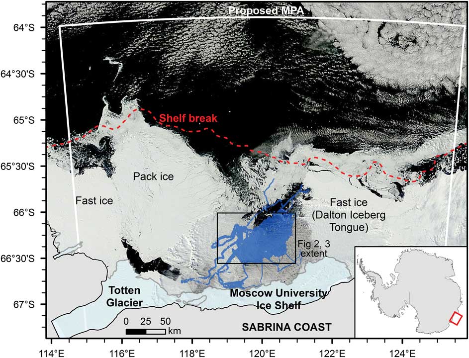
Fig. 1 MODIS satellite image from 26 February 2014 showing the sea ice distribution in the study region. The survey area (shown in blue) is located within the Dalton Iceberg Tongue polynya. MPA=marine protected area.
Physical setting
The Sabrina Coast includes the floating parts of the Totten Glacier tongue and the Moscow University Ice Shelf (Fig. 1). It contains extensive and persistent areas of fast ice along the western side of the Totten Glacier and to the east of the Moscow University Ice Shelf, forming the Dalton Iceberg Tongue (Fraser et al. Reference Fraser, Massom, Michael, Galton-Fenzi and Lieser2011). Prior to the US Antarctic Program NBP 14-02 research voyage, there had been no ship-based expeditions extending onto the continental shelf in this part of East Antarctica.
Sea floor bathymetry from the Sabrina Coast reveals a complex history of glaciation and deglaciation, with streamlined features and a series of recessional moraines evident (Leventer et al. Reference Leventer, Domack, Gulick, Huber, Orsi and Shevenell2014). Other features include bedforms in water depths of ~450 m, and a complex network of channels over crystalline bedrock in the southern part of the study area. The camera transects in this study targeted a number of these geological and glaciological features.
Modified Circumpolar Deep Water has been observed at depth along the continental shelf edge at ~119°E (Williams et al. Reference Williams, Meijers, Poole, Mathiot, Tamura and Klocker2011), and work is currently underway to determine areas where this water mass may flow onto the continental shelf. On the continental shelf, the Antarctic Coastal Current flows westward within 50 km of the coast, controlled by the strength of the east wind drift (Gwyther et al. Reference Gwyther, Galton-Fenzi, Hunter and Roberts2014). A large coastal polynya, the Dalton Ice Tongue polynya, is a recurrent feature west of the Moscow University Ice Shelf (Massom et al. Reference Massom, Reid, Stammerjohn, Raymond, Fraser and Ushio2013). Recent analysis of passive microwave data indicates that the polynya area varied by up to a factor of two between 1992 and 2008, with associated variations in the production of cold saline shelf waters proposed (Khazendar et al. Reference Khazendar, Schodlok, Fenty, Ligtenberg, Rignot and van den Broeke2013). Satellite sea ice information indicates that sea ice retreats from the north-east to the south-west, with all areas within the polynya typically ice-free by February (Massom et al. Reference Massom, Reid, Stammerjohn, Raymond, Fraser and Ushio2013). There is a short seasonal phytoplankton bloom associated with the sea ice breakup, with corrected satellite chlorophyll data (Johnson et al. Reference Johnson, Strutton, Wright, McMinn and Meiners2013) indicating that regional blooms may last from November to March. However,>70% of the measured chlorophyll flux is typically produced over ≤6 weeks between late December and mid-February.
Methods
Research was conducted aboard the RVIB Nathaniel B Palmer during NBP 14-02 (29 January to 16 March 2014) across a >3000 km2 area. A ‘yoyo’ camera, with downward facing digital still and video cameras mounted within a tubular steel frame, was deployed on a co-axial cable to image the sea floor; still images are presented here. The Ocean Imaging Systems DSC 10000 digital still camera (10.2 megapixel, 20 mm, Nikon D-80 camera) was contained within titanium housing. Camera settings were: F-8, focus 1.9 m, ASA-400. An Ocean Imaging Systems 3831 Strobe (200 W-S) was positioned 1 m from the camera at an angle of 26° from vertical.
A Model 494 bottom contact switch triggered the camera and strobe at 2.5 m above the sea floor, imaging ~4.8 m2 of sea floor. Parallel laser beams (10 cm separation) provided a reference scale for the images. During normal deployments, the live video feed was used to determine bottom contact, with the flash of the strobe light indicating the collection of an image. This mode allowed regular spacing between images of 10–20 m across the sea floor. Due to technical problems the final four deployments did not include a live video feed, relying instead on a contact alarm which sounded as soon as the bottom contact was activated on the sea floor. Occasional dragging of the bottom contact switch along the sea floor meant that the number of images collected and their spacing was not always known until the images were downloaded.
A total of 701 still images were analysed across ten transects (Table I). Transect lengths ranged from 400–1000 m, and were contained within a single habitat type as identified from the multibeam bathymetry. Images that were too close to the sea floor, and therefore poorly focussed, were discarded. Overlapping images were also discarded. Counts were corrected where sediment clouds produced from the bottom contact switch obscured part of the image, or removed where>30% of the image was affected. Post-processing of images involved colour correction in Adobe Photoshop to remove the blue bias. Images were then scored according to a combination of physical and biological properties. A grid was overlain on each image to assist in calculation of percent cover and to keep track of counts. Percent cover was recorded for substrate types (sand/mud, gravel, pebbles, cobbles, rock, boulders), occurrence of phytodetritus, presence of bioturbation features and overall biological cover by determining the number of grid squares covered by each of these and then calculating the overall percent occurrence. Due to the downward facing aspect of the camera, variations in relief could not be determined. Megafauna taxonomic groups were counted manually for the whole image according to the Collaborative and Automated Tools for Analysis of Marine Imagery (CATAMI) classification scheme (Althaus et al. Reference Althaus, Hill, Ferrari, Edwards, Przeslawski, Schönberg, Stuart-Smith, Barrett, Edgar, Colquhoun, Tran, Jordan, Rees and Gowlett-Holmes2015). This scheme is hierarchical and incorporates morphological characteristics for those taxa that have fine-scale features not easily distinguishable in imagery. Colonies of bryozoans, sponges and other colonial organisms were counted as individuals.
Table I Yoyo camera transects completed during NBP 14-02. Position is shown for the mid-point of each transect.

EOL=end of line, SOG=speed over ground, SOL=start of line.
In addition to the substrate properties derived from the image analysis, a range of environmental variables were included in statistical analyses (Table II). Rugosity and slope were calculated from the multibeam grid (Leventer et al. Reference Leventer, Domack, Gulick, Huber, Orsi and Shevenell2014) using the ArcGIS Benthic Terrain Modeler toolbox. Values for these parameters, as well as depth, were extracted for the mid-point of each transect as it was not possible to accurately calculate position for each image. The standard deviation of slope and rugosity was calculated within an 800 m radius to match the mean scale of the camera transects. Substrate types were divided into hard (< 80% mud/sand), mixed (80–99% mud/sand) and soft (100% mud/sand). These values were chosen to best represent the variability in substrate types given that most images had high mud/sand content, with<10% of the images characterized as hard and 35% as mixed.
Table II Additional physical datasets included in this study. Values were derived from the mid-point of each transect.

* Variable removed due to correlation>±0.95 with another listed variable.
Statistical analyses were completed in PRIMER v6 (Clarke & Gorley Reference Clarke and Gorley2006). Biological data were square root transformed prior to analysis to give more weighting to rare taxa and the similarity between observations was calculated using the Bray-Curtis similarity coefficient. Taxa diversity was calculated using formulas for Margalef’s richness, Pielou’s evenness, Shannon diversity (log base e) and Simpson diversity (1-λ’). A number of physical variables were log-transformed prior to analysis to reduce right skewed distributions, and one variable from each pair of highly correlated variables (R>0.95) was removed (see Table II). All physical variables were normalized to provide a common scale for analysis and similarity was calculated using Euclidean distance. The relationship between the distribution of taxa and environmental variables was tested using the BEST and principle co-ordinates analysis (PCO) functions in PRIMER, with Spearman rank correlations indicating the strength of the relationships. A permutation test (999 permutations) was used to test the significance of the biophysical relationships. A one-way ANOSIM was used to test for differences in taxa abundance and composition between substrate types, and between transects on the same substrate type. These analyses allowed us to test the null hypothesis that the presence of boulders and dropstones has no significant effect on the diversity, abundance and composition of the benthic biota.
Results
Characteristics of the physical environment
Sea bed imagery was used to determine substrate characteristics along each transect. All transects were dominated by muddy/sandy substrates, with nine of the ten transects also containing varying proportions of hard substrates in the gravel to boulder size range (Fig. 2). Transects 10, 20, 35, 36, 50 and 52 all contained a small proportion of boulders, which were deposited on the sea floor as dropstones; dropstones were scattered throughout the transects. Smaller boulders were often partially buried in sediment and many of the larger boulders in deeper water appeared to have a manganese oxide coating. Transect 34 contained a relatively high proportion of gravel in addition to some dropstones. Manganese coatings were absent from the boulders on this shallower transect. Transects 47 and 49 were located on crystalline bedrock and contained the highest proportions of hard substrates. Both of these transects had an average cover by boulders of 17 percent, with cobbles, pebbles and gravel adding an additional 9% (Transect 49) to 19% (Transect 47). Transect 47 also contained an average of 5% bedrock cover.
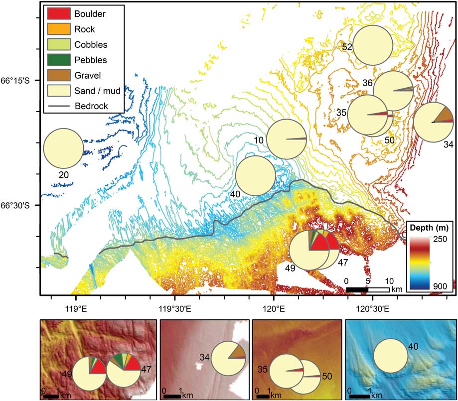
Fig. 2 Percent cover of substrate types averaged within each transect. Note that boulders on Transects 20 and 52 have occurrences of<0.2%, so are not visible on the pie charts. Insets show enhanced views of selected transects over multibeam bathymetry data.
Depth, slope and rugosity values were derived from the multibeam bathymetry grid and analysed to understand variations between and within each transect. Depth for the study ranged from 274 m (Transect 34) to 896 m (Transect 20). Depth ranges within each transect were generally small (< 20 m), with a slightly larger range along Transect 36 (30 m) associated with a moraine feature and Transect 49 (53 m) due to a steep slope associated with the edge of a bedrock channel. Slope values were generally<5°, but reached 45° along the channel flank on Transect 49. Rugosity was also highest along the channel edge, with some higher values also associated with the bedrock plateau on Transect 47. Low rugosity occurred on each of the other transects. While iceberg scours were visible on the multibeam imagery at depths of≤500 m, they were not observed along any of the transects.
Characteristics of the benthic assemblage
A total of 68 different megafaunal taxa were observed across the study area (Table III). Of these, brittle stars and polychaete tubeworms were the most abundant (Table IV); brittle stars were observed in every image. Seven taxa were observed in>50% of the images, with the remaining taxa occurring more sporadically and several only observed once or twice.
Table III List of all taxa observed and identified according to the CATAMI scheme (Althaus et al. Reference Althaus, Hill, Ferrari, Edwards, Przeslawski, Schönberg, Stuart-Smith, Barrett, Edgar, Colquhoun, Tran, Jordan, Rees and Gowlett-Holmes2015) and their total abundance.

Table IV Most abundant megafaunal taxa across the study area, with average and maximum numbers of individuals m-2 and percent occurrence across all images. Numbers in brackets indicate the transect on which the maximum number for that taxa occurred.

The relative abundance of taxa averaged within each transect indicates that while brittle stars dominated on most transects, there was significant variability in the assemblage composition (Fig. 3a). Brittle stars reached highest proportions on Transects 10 and 20, while lowest abundances occurred within Transects 34 and 47. These two transects had relatively high abundances of polychaete tubeworms, sponges (mostly ball sponges, with high abundance of massive sponges along Transect 34 and hollow sponge tubes along Transect 47) and bryozoans (mostly hard branching). Lower abundances of brittle stars also occurred within Transect 52, with relatively high abundances of crustaceans (mostly amphipods), holothurians (mostly mobile forms living on the substrate), anemones and stalked colonial ascidians. Adjacent Transects 35, 50 and 36 (all within 8 km) had a similar overall composition. Transects 47 and 49 were also located within 2 km of each other, yet their overall abundances revealed significant differences, including the relative abundances of sponges, brittle stars, brachiopods and bryozoans. Representative images are included in Fig. 4.

Fig. 3a Relative abundance of taxa averaged within each transect. Insets show enhanced views over multibeam bathymetry for selected transects. b. Average values for Shannon diversity, individuals m-2, and percent biological cover for each transect. The individuals m-2 range from 8 (Transect 52) to 60 (Transect 47), while percent biological cover ranges from 5 (Transect 40) to 52 (Transect 47).

Fig. 4 Representative taxa on sea floor transects for soft (a., f.), mixed (b.) and hard substrates (c., d., e.). A=anemone, A-sc/A-uns=ascidian, stalked colonial/unstalked solitary, B=brachiopod, Bs=brittle star, B-hb/B-en/B-sd/B-sf=bryozoan, hard branching/encrusting/soft dendroid/soft foliaceous, C-un=crinoid, unstalked, F=fish, G-bbs/G-f=gorgonian bottle-brush, simple/fan, H-if/H-iv/H-m=holothurian infaunal/on invertebrate/mobile, Hy-b=hydrocoral, branching, Hy-cf=hydroid, colonial feathered, PD=phytodetritus, Pt=polychaete tube, S-b/S-bl/S-eb/S-en/S-es/S-t=sponge, barrel/ball/erect branching/encrusting/erect simple/tube, Sp=sea spider. Scale bars indicate 10 cm.
Abundance and diversity of taxa revealed significant variability between transects. The highest average number of individuals m-2 (60) and percent biological cover (52%) occurred on Transect 47, and high values also occurred on Transects 34 and 49 (Fig. 3b). Relatively low values were observed on other transects (8–23 ind. m-2 and 5–10% cover). Shannon diversity of the taxa was highest on Transects 47 and 34 (2.4 and 2.0), with high values also recorded for Transect 36 (1.9). Lowest taxa diversity occurred on Transects 10, 40 and 20 (1.2, 1.1 and 0.7).
Relationship to environmental variables
The association between the physical variables and the composition and abundance of the taxa was explored using the PRIMER 6 software. The BEST routine indicated that water depth, latitude and percent cover by boulders and phytodetritus were most strongly correlated (ρ=0.592, P<0.001) with the abundance of taxa across the datapoints. A PCO plot (Fig. 5a) was used to indicate how physical variables were distributed in relation to the assemblage data. Axis 1 reflected the distribution of phytodetritus and soft substrates in the negative direction and boulders and gravel in the positive direction, explaining a total variation of just over 30% (Fig. 5a). Axis 2 explained 14% of the variation, with latitude distributed in the negative direction and depth and chlorophyll in the positive direction. Deeper depths, greater phytodetritus and muddy/sandy substrates were associated with lower abundance (Fig. 5b) and lower Shannon taxa diversity (Fig. 5c), while harder substrates (e.g. boulders and gravelly sediments), shallower depths and decreasing phytodetritus were associated with high abundance (Fig. 5b) and higher Shannon taxa diversity (Fig. 5c). The harder substrates with a more diverse assemblage were comprised of taxa including brachiopods, hard bryozoans, polychaete tubeworms, sponges (particularly ball, massive and encrusting sponges) and sea whips (Fig. 5b). Higher abundances of mobile holothurians and amphipods were associated with muddy/sandy substrates with greater phytodetritus, while taxa such as brittle stars, irregular urchins and anemones were associated with all substrates.
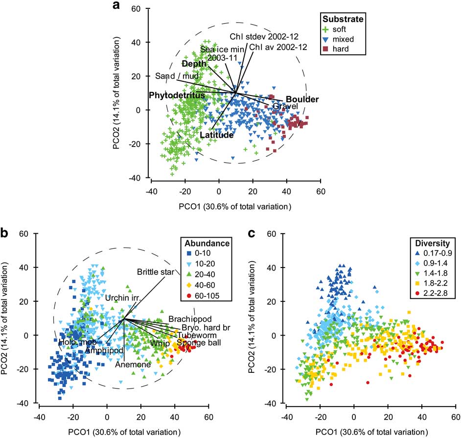
Fig. 5 Principle co-ordinates analysis of assemblage counts. a. Symbols represent substrate type with Spearman rank correlation of physical variables overlain as vectors. Variables in bold text have the highest combined correlation (0.592, P<0.001) against the assemblage counts using the BEST routine. b. Symbols indicate the number of individuals (m-2) at each datapoint with Spearman rank correlation of key taxa overlain as vectors. c. Symbols represent the Shannon diversity of taxa at each datapoint.
Habitat heterogeneity
The occurrence and impact of habitat heterogeneity was explored for hard versus soft substrates along each transect to test the null hypothesis that boulders and dropstones have no significant effect on the diversity, abundance and composition of the benthic biota. Dropstones occurred on seven Transects (10, 20, 34, 35, 36, 50 and 52), while crystalline bedrock along Transects 47 and 49 created abundant hard substrates.
Substrate types, based on percent cover, were assigned to the categories soft, mixed and hard categories. ANOSIM analysis indicated that the composition and abundance of taxa was significantly different between substrate types (ANOSIM global R=0.477, P<0.001; soft vs hard R=0.868, P<0.001), as were the measures of taxa diversity (ANOSIM global R=0.407, P<0.001; soft vs hard R=0.767, P<0.001). A PCO plot indicated a distinct clustering of the taxa according to substrate characteristics, with only slight overlap between categories (Fig. 5a). The abundance and diversity of taxa (Fig. 5b & c) also showed a gradational change in values consistent with changing substrate type (Fig. 5a).
Pie charts of key taxa within hard and soft substrate types indicated that brittle stars and polychaete tube worms were the most abundant taxa across all substrates. Hard substrates were dominated by sessile suspension feeders (58%), including hard branching bryozoans, brachiopods, encrusting bryozoans and ball sponges (Fig. 6a & b). Soft substrates had high abundances of mobile taxa (84% overall), including almost 50% brittle stars, amphipods and mobile holothurians, and some sessile suspension feeders such as anemones and infaunal holothurians. Hard substrates were inhabited by an average of five times as many individuals as soft substrates, with over twice the taxa richness and significantly higher values for the other diversity measures (Fig. 7). The percent biological cover was also significantly different between substrate types, with six times the biological cover on hard compared to soft substrates. Values for areas of mixed substrate fell halfway between those of hard and soft substrates.
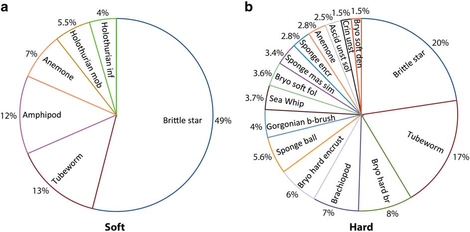
Fig. 6 Composition of most abundant taxa up to 90% total abundance for a. soft and b. hard substrates.
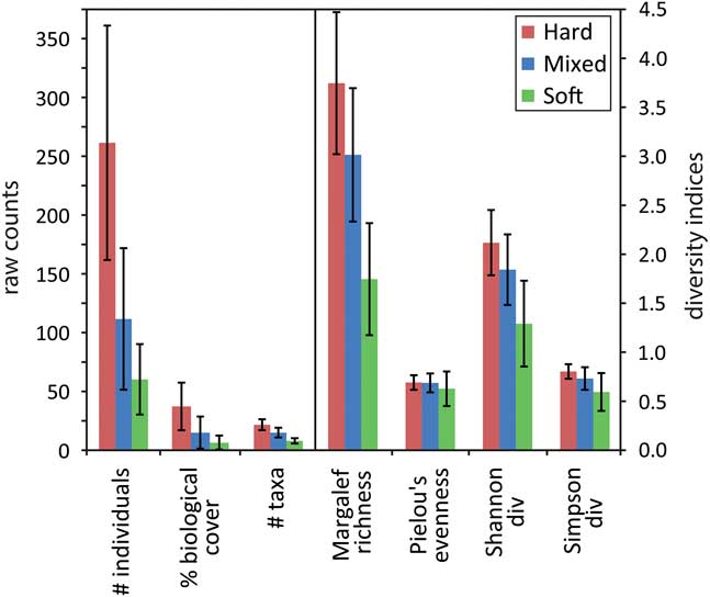
Fig. 7 Average abundance, cover and diversity indices according to substrate type, with standard deviation indicated by the bars. Note the change in scale from the left to right.
ANOSIM analysis of differences between transects for taxa abundance on hard and mixed substrates indicated a significant difference between transects (Global R=0.488, P<0.001); however, there was a large range in R values between individual transects. Taxa on Transects 35, 50 and 36 showed the greatest overlap in taxa abundance and composition (Fig. 8a; ANOSIM R=0.121–0.147). These transects were all located within 8 km of each other and can be considered as a single habitat: Habitat A. Less similarity was observed between the remaining transects, with the multidimensional scale (MDS) plot illustrating the distinct separation between Transects 34, 47 and 49 (ANOSIM R=0.421–0.592), which were located on a relict moraine and crystalline bedrock, respectively. Transects 10, 20 and 52 had a broad distribution on the MDS plot, with some overlap with Transect 49. Depth was associated with some of the assemblage variability in areas of hard and mixed substrates, with shallow transects (275–315 m; Transects 34 and 47) separated from deeper transects (Fig. 8b). There is no clear relationship between depth and the average counts of individuals m-2 (Table V).
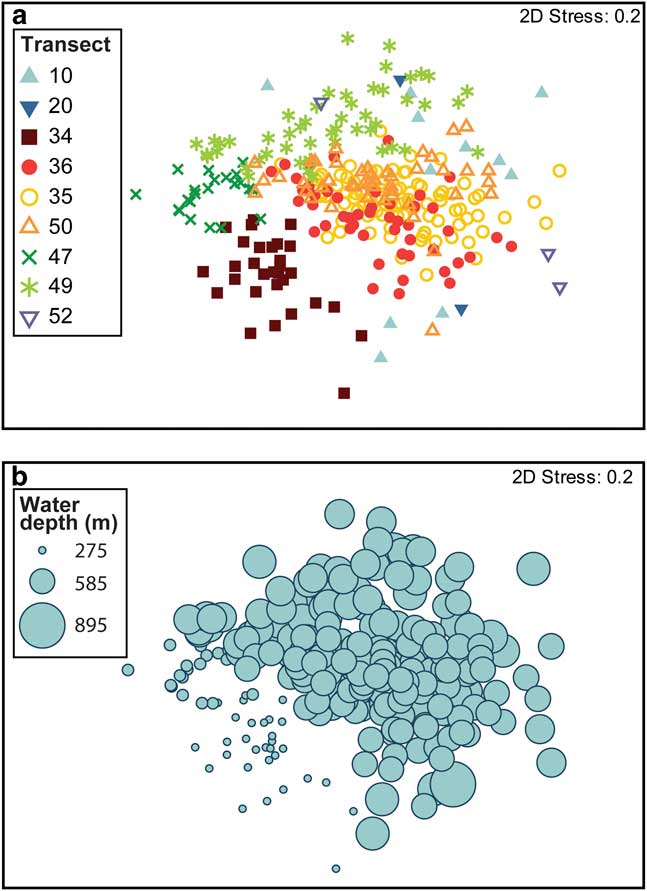
Fig. 8 Multidimensional scale plot of taxa abundance and composition based on Bray-Curtis similarity across hard and mixed substrates. a. Symbols represent transects. b. Symbol size indicates water depth.
Table V Percent abundance and average count of individuals m-2 for taxa found only on hard substrates. Transects are labelled according to their locality. Transect 40 is not shown as it contained no hard substrates.

Eight taxa were found primarily on hard substrates with a restricted distribution between transects (Table V). Branching hydrocorals and smooth barrel sponges were only found on hard substrates associated with crystalline bedrock and a relict moraine, while the remaining taxa were also found within Habitat A, and in relatively low abundances on Transect 10. Each of these taxa were absent from those transects most distal to the other sites (Transects 20 and 52, which consisted of<1% hard substrates).
Data from Transect 50 was used to illustrate how substrate and diversity indices vary (Fig. 9). Images in which there was high cover by hard substrates (> 15%) indicated dramatic increases in the number of individuals present and the Shannon diversity compared to surrounding images with much lower occurrences of hard substrates. This pattern of higher diversity and number of individuals was observed even when the cover by hard substrates increased by just a few percent. Individual boulders on images typically had a dense invertebrate cover, amidst softer substrates with a relatively sparse biological cover, thus creating habitat heterogeneity on a submetre scale.
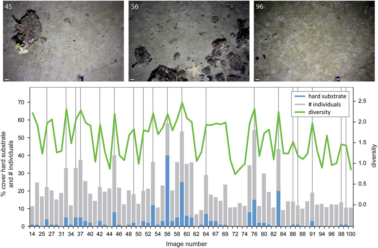
Fig. 9 The percent cover of hard substrate is associated with changes in the number of individuals and Shannon diversity along Transect 50. Representative examples of sea floor images are shown, numbered according to image number, with a 10 cm scale bar. Images were selected to highlight a range of different taxa colonizing the hard substrates and to show examples of mixed hard and soft substrates in a single image.
Discussion
Understanding the Sabrina Coast sea floor environment and assemblages
Substrate type and water depth have frequently been associated with the distribution of benthic biota on continental shelves, including the Antarctic shelf (e.g. Jones et al. Reference Jones, Bett and Tyler2007, Post et al. Reference Post, Beaman, O’Brien, Eléaume and Riddle2011, Smith et al. Reference Smith, O’Brien, Stark, Johnstone and Riddle2015), and these factors (specifically boulders and water depth) were also among the most significant factors relating to the distribution of benthic taxa in this study. Coarse substrates provide a hard attachment and an elevated position off the sea floor, enhancing the food supply for sessile suspension feeders (Starmans et al. Reference Starmans, Gutt and Arntz1999), while deposit feeders are often associated with soft substrates where they are able to feed on fine particles (Jones et al. Reference Jones, Bett and Tyler2007). These patterns create distinct differences in assemblages occurring on hard and soft substrates. The strong relationship with substrate is in contrast to studies in areas strongly influenced by ice disturbance, in which substrate has been found to be of lesser importance (Gutt Reference Gutt2007). Ice disturbance due to scouring was not observed within any of the Sabrina Coast shelf transects, allowing the effects of substrate to be clearly discerned. The association with depth may reflect other factors, such as organic matter flux, temperature, salinity and oxygen content.
In addition to substrate type and depth, phytodetritus cover and latitude were shown to be important factors associated with the distribution of the benthic taxa. The accumulation of phytodetritus results in the local enhancement of deposit feeding communities (Fig. 5b). The highest accumulation of phytodetritus on the sea floor occurs in areas of bottom water recirculation and sediment focusing of muddy/sandy sediments (Fig. 5a). Phytodetritus cover in the current study is not strongly correlated with satellite surface chlorophyll measurements. This suggests that, at a local scale, there is weak spatial bentho-pelagic coupling in this system, with accumulation of phytodetritus most probably dependent on redistribution via bottom currents. The effect of zooplankton grazing on phytodetritus flux is considered to be minimal in the bloom/bust setting of polynyas (Grebmeier & Barry Reference Grebmeier and Barry2007), and satellite ocean colour observations from the Dalton Iceberg Tongue polynya indicate a typical bloom period of only six weeks, which further reduces the opportunity for significant grazing.
Sub-bottom profiles over the transects indicate that the surface sedimentary drape is very thin (typically<4 m; Leventer et al. Reference Leventer, Domack, Gulick, Huber, Orsi and Shevenell2014) even in areas of sediment focusing. The presence of manganese oxides on dropstones across the deeper parts of this continental shelf further suggests low sedimentation rates (see Wright et al. Reference Wright, Graham, Chang, Choi and Lee2005 and references therein). Low sedimentation rates may reflect low surface production or low accumulation of phytoplankton on the sea floor, but it may also be that the pelagic deposition is rapidly scavenged by the mobile deposit feeding brittle stars, holothurians and amphipods, leaving little to accumulate on the sea floor. Surface deposit feeders can respond rapidly to the arrival of phytodetritus at the sea floor, with observations of megafaunal activities on the north-east Atlantic sea floor indicating the removal of deposits within six weeks of arrival (Bett et al. Reference Bett, Malzone, Narayanaswamy and Wigham2001), while elasipod holothurians on the western Antarctic Peninsula (WAP) increase their feeding rates by a factor of more than two during periods of high phytodetritus flux (Sumida et al. Reference Sumida, Bernardino, Stedall, Glover and Smith2008). The association between mobile taxa and phytodetritus in this study, and the low sediment accumulation, is consistent with the rapid response of the benthos to this food source.
Latitude was also shown to be a significant factor associated with the distribution of the benthic taxa. In this setting, latitude shows partial negative correlation to a number of variables, including: sea surface chlorophyll, sea floor rugosity and slope. A combination of these factors may result in the association between the faunal distributions and latitude. Alternatively, the latitudinal distribution of transects may represent another environmental gradient not measured in this study.
Comparison to taxa on other Antarctic shelf environments
The abundance of megafauna taxa on the Sabrina Coast sea floor is generally high relative to other locations on the Antarctic continental shelf where still imagery has been analysed (Table VI). Abundances are particularly high compared to those observed on the WAP shelf (Sumida et al. Reference Sumida, Bernardino, Stedall, Glover and Smith2008), in the Amundsen and Bellingshausen seas (Starmans et al. Reference Starmans, Gutt and Arntz1999), and the Fimbul Ice Shelf region, Weddell Sea (Jones et al. Reference Jones, Bett and Tyler2007). Similar average abundances are observed between this study and those on the western Ross Sea shelf (Barry et al. Reference Barry, Grebmeier, Smith and Dunbar2003) and in the WAP fjords (Grange & Smith Reference Grange and Smith2013), while much higher abundances have been observed on the Weddell Sea shelf (Gutt & Starmans Reference Gutt and Starmans1998).
Table VI Comparison of abundance and key taxa based on photographic studies at comparative depths on Antarctica’s continental shelf. Mean abundances of megafauna are shown in brackets.

The relatively high abundances of megafauna in this study may reflect the generally higher productivity associated with polynyas; the Dalton Iceberg Tongue polynya is a recurrent feature of the Sabrina Coast (Massom et al. Reference Massom, Reid, Stammerjohn, Raymond, Fraser and Ushio2013). Polynyas significantly enhance benthic production in both the Arctic and Antarctic environments due to the high export production from the surface waters (Grebmeier & Barry Reference Grebmeier and Barry2007). While we observed weak bentho-pelagic coupling on a local scale, surface production is likely to significantly influence benthic production on a regional scale, as also observed in studies within the Ross Sea polynya, where benthic productivity within the polynya was significantly higher than in ice-covered areas (Grebmeier & Barry Reference Grebmeier and Barry2007). However, Antarctic polynya primary and benthic production is quite variable due to differences in water depth and grazing pressure. These sources of variability complicate the interpretation of regional abundance patterns.
A circumpolar distribution has been observed for many Antarctic species across various taxonomic groups (Griffiths et al. Reference Griffiths, Barnes and Linse2009), but at an assemblage level there are significant regional differences that depend on a range of physical factors (see review by Convey et al. Reference Convey, Chown, Clarke, Barnes, Bokhorst, Cummings, Ducklow, Frati, Green, Gordon, Griffiths, Howard-Williams, Huiskes, Laybourn-Parry, Lyons, McMinn, Morley, Peck, Quesada, Robinson, Schiaparelli and Wall2014), disturbance regimes (Barnes & Conlan Reference Barnes and Conlan2007) and potentially ongoing post-glacial recolonization (Gutt Reference Gutt2006). The Sabrina Coast megafaunal composition is most similar to that observed in the Fimbul Ice Shelf region (Table VI; Jones et al. Reference Jones, Bett and Tyler2007), with brittle stars and polychaetes most abundant in each system. Brittle stars are also one of the key taxa in the western Ross and Weddell seas (Gutt & Starmans Reference Gutt and Starmans1998, Barry et al. Reference Barry, Grebmeier, Smith and Dunbar2003). In the Ross Sea, brittle star and worm-dominated assemblages are associated with deep slopes (500–600 m) and basins (700–900 m), while high densities of sponges and crinoids are associated with dropstones in the deeper basins (Barry et al. Reference Barry, Grebmeier, Smith and Dunbar2003), consistent with our observations. There is less similarity between the megafauna in this study and that observed in the WAP and the Amundsen and Bellingshausen seas. Polychaetes are a key taxon in the WAP fjords and on the Sabrina Coast, but abundance of brittle stars is much lower in the WAP (Grange & Smith Reference Grange and Smith2013). The dominance of brittle stars and polychaetes in the Sabrina Coast study region reflects the dominance of soft substrates (> 90% of images), with bryozoa and other sessile invertebrates almost exclusively restricted to dropstones and the nearshore crystalline bedrock. Brittle stars are also relatively abundant in other East Antarctic settings, including the Ross and Weddell seas, but they are much less abundant in West Antarctic sites, including the WAP and Amundsen Sea. The West Antarctic studies indicate a much more variable assemblage than that seen in the East Antarctic studies.
Habitat heterogeneity as diversity hotspots on the continental shelf
The importance of fine-scale habitat heterogeneity in enhancing diversity has been established in several shelf settings (e.g. Hewitt et al. Reference Hewitt, Thrush, Halliday and Duffy2005, Thrush et al. Reference Thrush, Hewitt, Cummings, Norkko and Chiantore2010), with dropstones noted as a habitat for sessile invertebrates in both the Antarctic and Arctic (Starmans et al. Reference Starmans, Gutt and Arntz1999, Schulz et al. Reference Schulz, Bergmann, von Juterzenka and Soltwedel2010). The current study demonstrates that habitat heterogeneity on a small scale can be important for the overall biodiversity of a system. Dropstones were associated with a significant increase in the composition, abundance and diversity of taxa on a submetre scale, with particularly high abundances of sessile invertebrates (e.g. bryozoans, sponges, gorgonians and ascidians), and several other hard substrate taxa. Given that the majority of the Antarctic shelf is<200 m and dominated by muddy sediments (Smith et al. Reference Smith, Mincks and DeMaster2006), the importance of dropstones in providing hard substrates for sessile invertebrates cannot be underestimated.
The present dataset allows us to consider the role of dropstones as potential stepping stones for the dispersal of sessile suspension feeders across the Sabrina Coast shelf. Our ANOSIM analysis revealed significantly greater variability between, rather than within, substrate types. This finding suggests that, at the taxa level, there is a high degree of connectivity between hard substrate areas. There were only eight taxa associated with hard substrates that were found to have a restricted distribution. Two of these taxa were found only on nearshore transects, while the other six were associated with the crystalline bedrock, a relict moraine and Habitat A environments, but were absent or had generally low abundance on the most distal transects. These results suggest that these eight taxa may have more limited dispersal capability, or that they are restricted in their distribution by the absence of optimal habitats or by competition. It is not possible to fully assess the impact of these different factors, but some general observations can be made. The branching hydrocorals were limited to just the three transects associated with the crystalline bedrock and relict moraine and are known to have very localized dispersal capability (Cairns Reference Cairns2011). Their localized dispersal may explain their absence in areas further offshore where dropstones have a more scattered distribution. The smooth barrel sponges (Anoxycalyx joubini (Topsent); Fig. 4d; Downey, personal communication 2015) were also only observed along the two shallowest transects. On the Antarctic margin, this sponge is only known from water depths of 40–400 m, so its absence across other transects, which are all>440 m, may be due to depth limitation for this species. The remaining hard substrate taxa (Table V) do not show any clear limitation with water depth to 600 m. The broad distribution of the majority of taxa across hard substrates (within an area of 800 km2) indicates that there is a sufficient density of dropstones for most sessile invertebrates to disperse across the region. The occurrence of dropstones and other hard substrates across different habitats (shallow areas through to deep basins) therefore adds considerably to the overall diversity of taxa and their distribution across the Sabrina continental shelf.
The association of sessile invertebrates and dropstones has a cumulative effect on the diversity of regional hard substrate assemblages. The high diversity and abundance of taxa found on hard substrates is enhanced by the 3-D surface created by the organisms themselves, particularly sponges, gorgonians and bryozoans, which form complex habitats for other invertebrates. The images in Fig. 4b & d show crinoids perched on the top of the sponges and a fish within a barrel sponge, while crinoids, brittle stars and a holothurian are also visible on the edges of the bottle-brush gorgonians (Fig. 4c & d). A wide variety of invertebrates are also known to inhabit the canals of sponges, which provide protection from predators and strong currents, and also a detrital food supply (Buhl-Mortensen et al. Reference Buhl-Mortensen, Vanreusel, Gooday, Levin, Priede, Buhl-Mortensen, Gheerardyn, King and Raes2010). The 3-D structure of these organisms thereby acts to further enhance the local diversity in areas of dropstones.
Conclusions
Understanding the relationships between physical parameters and the distribution and abundance of benthic taxa is important for improving our understanding of the factors that drive biodiversity and species distribution on the Antarctic shelf. Benthic assemblages vary considerably between regions on the Antarctic margin, as do the factors that drive their distribution. Because the Sabrina Coast shelf is relatively undisturbed by the impact of icebergs, we were able to explore the impact of other physical factors on the benthos. The distribution of taxa on this shelf is correlated with substrate properties, water depth, phytodetritus accumulation and latitude. Substrate properties vary over fine geographical scales due to the scattered distribution of dropstones, which create hotspots in both the abundance and diversity of sessile suspension feeding taxa. The habitat heterogeneity created by dropstones significantly enhances the diversity and biomass of the benthic community across this shelf, with several taxa found only on hard substrates. The relatively high regional abundance of benthic taxa, represented by a diverse range of taxa, strengthens the case for protecting this area in the network of MPAs proposed for East Antarctica. This dataset provides a snapshot of the current status of this ecosystem, which can be used as a baseline for monitoring any ecosystem change that may occur due to future natural or anthropogenic change.
Acknowledgements
Our thanks to the captain, crew and USAP Nathaniel B. Palmer NPB 14-02 Shipboard Science Party. A special thanks to the ASC staff, including Barry Bjork and Sheldon Blackman, for their technical assistance in setting up and repairing the ‘yoyo’ camera. We thank Rachel Downey, Rachel Przeslawski and Andrew Carroll for assistance with biological identifications, and Andrew Carroll and Floyd Howard for their comments on an earlier version of the manuscript. Jackie Grebmeier and an anonymous reviewer are thanked for their constructive reviews. This project was supported by NSF Office of Polar Programs grants ANT-1143834, 1143836, 1143837, 1143843 and 1313826. ALP publishes with the permission of the Chief Executive Officer, Geoscience Australia.
Author contributions
All authors have contributed to this manuscript. ALP characterized the sea floor images, completed statistical analyses and wrote the paper. CL processed the multibeam bathymetry data and assisted with data interpretation. EWD assisted with survey design, collection of imagery and data interpretation. AL was the field survey leader and contributed to collection of imagery and data interpretation. AS contributed to the preparation of the paper and data interpretation. ADF contributed sea ice data, analysis and interpretation. The NBP 14-02 Science Team are acknowledged for their contribution to the collection of the sea floor images and physical datasets.


