


INTRODUCTION
The new stylized fact of American politics is that the wealthy dominate American democracy. A growing body of political science research concludes that government policy is far more responsive to the preferences of the affluent than to those of either the middle class or poor (Bartels Reference Bartels2008; Ellis Reference Ellis2012, Reference Ellis2017; Gilens Reference Gilens2005, Reference Gilens2012; Gilens and Page Reference Gilens and Page2014; Hayes Reference Hayes2013; Rigby and Wright Reference Rigby, Wright, Enns and Wlezien2011; Tausanovitch Reference Tausanovitch2016). Gilens, for example, concludes that “the preferences of the vast majority of Americans appear to have essentially no impact on which policies the government does or doesn’t adopt” (Reference Gilens2012, 1). Such class-based distortion violates norms of equal voice and, worse still, raises the spectre of a vicious cycle in which low-income individuals are locked out of power, in which economic inequality begets political inequality which begets still more economic inequality. This is the warning of the “economic elite domination model” (Gilens and Page Reference Gilens and Page2014).
Claims of class-based inequality in responsiveness have not gone unchallenged. Some studies find evidence against the basic result (e.g., Bhatti and Erikson Reference Bhatti, Erikson, Enns and Wlezien2011; Soroka and Wlezien Reference Soroka and Wlezien2008; Ura and Ellis Reference Ura and Ellis2008; Wlezien and Soroka Reference Wlezien, Soroka, Enns and Wlezien2011). Others argue that the implications of unequal responsiveness are overstated. For example, Enns (Reference Enns2015a, Reference Enns2015b) notes that low- and middle-income individuals receive a great deal of coincidental representation even when politicians respond primarily to the affluent, because preferences tend to differ little by income group. Branham, Soroka, and Wlezien (Reference Branham, Soroka and Wlezien2017) find that the ideological impact of affluent influence is attenuated because well-to-do constituents have a mix of both liberal and conservative preferences. This important research skeptical of affluent influence has perhaps received less attention (scholarly or otherwise) than the work of Bartels or Gilens, and there remain unresolved debates regarding the nature, pervasiveness, and substance of such influence (see generally Erikson Reference Erikson2015).
Independent of these debates, there is also a growing concern that elected officials care “too much” about the opinions of their copartisans or electoral base, creating a partisan distortion in representation (Clinton Reference Clinton2006; Kastellec et al. Reference Kastellec, Lax, Malecki and Phillips2015; Shapiro et al. Reference Shapiro, Brady, Brody and Ferejohn1990; Warshaw Reference Warshaw2012). This bias can arise from a variety of factors, most prominently the need to win primary elections (Clausen Reference Clausen1973; Fenno Reference Fenno1978; Gerber and Morton Reference Gerber and Morton1998). Such a bias can pull policy away from the relatively moderate preferences of the median voter, toward the more ideologically extreme preferences of partisans. As with the economic distortion, a partisan distortion in representation violates norms of equal voice and can also become reinforced and entrenched (in this case through the manipulation of electoral rules, gerrymandering, and the like). This partisan distortion is also increasingly invoked as conventional wisdom, but rigorous empirical investigations of partisan biases in representation remain (at least relative to studies of affluent influence) both uncommon and somewhat limited in scope.
As work in this vein continues, scholars are finding evidence of other partisan distortions. One is that parties might not behave symmetrically with respect to constituent opinion. Some research suggests that Democratic and Republican lawmakers do not put the same weight on opinion (Clinton Reference Clinton2006; Krimmel, Lax, and Phillips Reference Krimmel, Lax and Phillips2016). Another is these lawmakers may discount opinion to vote the “party line” and thereby further their party’s legislative agenda (Hussey and Zaller Reference Hussey, Zaller, Enns and Wlezien2011), which itself may not reflect public opinion (Achen and Bartels Reference Achen and Bartels2016). As with economic distortions, there remain significant unresolved debates regarding the scope and strength of partisan distortions.
Perhaps surprisingly, research on class-based and partisan distortions in representation has proceeded on two, largely separate, tracks. We argue, however, that existing debates cannot be resolved without simultaneously considering both types of distortions. A failure to do so risks over- or underestimating the prevalence of each and obscures interactions between them. For example, copartisan pull might constrain affluent influence or vice versa. Alternatively, partisanship might be the vehicle through which affluent influence operates. What might appear to be over-responsiveness to the preferences of the rich could simply be coincidental, if copartisan opinion and the rich opinion tend to agree. Moreover, potential distortions in representation may manifest differently in the behavior of Democratic and Republican lawmakers.
We juxtapose and integrate economic and partisan biases in the study of representation, thereby assessing whether these forces are indeed coincidental, complementary, constraining, or conflicting. Our efforts simultaneously serve as both the first study of economic distortions to foreground partisan opinion and the first study of partisan distortions to foreground affluent opinion.
Our analysis is the most revealing when potential influences on lawmakers conflict, and elected representatives have to take sides. What happens when party and purse pull in opposite directions, when a lawmaker’s copartisan constituents and rich constituents want different things? What happens when copartisans side with rich against poor or vice versa? What happens when there is intraparty conflict between rich and poor opinion? Taking up the complications noted by Krimmel, Lax, and Phillips (Reference Krimmel, Lax and Phillips2016) and others, do the two parties respond to opinion and deal with cross pressures the same way? Do pressures to vote the party line lead lawmakers to ignore the preferences of key constituents altogether?
We build on significant work by others, confronting many of the same challenges they did, but utilizing different solutions. These solutions require knowing the preferences on specific issues, not only of the rich and poor but also of partisan groups and of income groups within each party. We need a sufficient number and variety of roll call votes, not only for generalizability but also so that we have sufficient instances of subconstituency disagreement to disentangle competing influences.
We obtain all this using a large quantity of survey data, along with the most recent advances in subgroup opinion estimation. Our dyadic analysis of representation in the US Senate uses 49 roll call votes from eight sessions of Congress (2001–15). The votes we utilize include some of the most important economic, social, and foreign policy votes cast by members of Congress during this period (e.g., health-care reform, President Obama’s stimulus bill, an extension of the Bush tax cuts on capital gains, the Federal Marriage Amendment, and a vote to withdraw American military personnel from Iraq). We use and extend multilevel regression and poststratification (MRP) to create the necessary estimates of public opinion for partisan and class subgroups and incorporate uncertainty around our opinion estimates.
Our baseline “taking sides” analyses reproduce the foundational findings of the economic and partisan distortion literatures, but using different and more recent evidence. We find that the affluent are more likely than the poor to get what they want, especially when each group desires a different policy (not that this is common). And, we find that lawmakers more frequently vote in a manner that is consistent with the preferences of their home-state copartisans than with their median constituent. We also uncover, consistent with Krimmel, Lax, and Phillips (Reference Krimmel, Lax and Phillips2016), broad evidence of asymmetric responsiveness, with Democratic senators far more responsive to opinion in general than their Republican colleagues. However, when we consider partisan and elite opinion in tandem, our results depart from the conventional wisdom, especially in regards to affluent influence. Our results show that affluent influence is largely a story of partisan politics. It both works through and is limited by partisanship.Footnote 1
Republican senators are, on average, more responsive to the rich than the poor, but Democratic senators are largely more responsive to the poor than rich, particularly when there is class conflict. Thus, it is Republican senators, not Democrats, who are primarily responsible for the overall pattern of affluent influence. This does not, however, mean that Democrats are entirely “innocent.” In a small subset of votes in which well-to-do Democrats prefer a different policy than poor or middle-class Democrats, Democratic senators are somewhat more likely to side with the affluent. That said, in that type of situation, Republican senators side far more with the Republican rich over Republican poor.
How does this revised sense of affluent influence stand up against partisanship directly? It does not—party trumps the purse. Senators of both parties are far more responsive to copartisan opinion than rich opinion. When the two conflict, senators of both parties tend to side overwhelmingly with their copartisans over the rich.
This partisan effect not only sharply limits affluent influence but also seems to largely account for its existence in the first place. Republican copartisan opinion is more likely to align with the opinions of the rich than with those of the poor (whereas Democratic copartisan opinion is more likely to align with poor). So when Republicans vote in the manner preferred by their copartisan constituents back home, these senators are also providing coincidental representation to the affluent more than the poor. When Democrats listen to their partisan constituents, coincidental representation favors the poor over rich.
There is, as noted above, yet another partisan constraint on affluent influence. Pressure to vote the party line seems to trump responsiveness to opinion of any type. Even Republicans—who tend to side with the rich over poor, and Republican constituents over rich—will side with their fellow Republican senators against rich, against Republicans constituents, or both combined.
In sum, our analyses yield a fundamentally different understanding of the democratic deficit in legislative representation—and of affluent influence.
THINKING ABOUT REPRESENTATION
Economic Distortions of Representation
The seminal contributions on affluent influence are Bartels (Reference Bartels2008) and Gilens (Reference Gilens2005, Reference Gilens2012). Bartels studied the roll call voting behavior of individual senators, using as dependent variables the overall ideological tenor of a senator’s voting record (measured using the W-Nominate scores of Poole and Rosenthal Reference Poole and Rosenthal1997) as well as individual votes on eight bills, half of which addressed abortion. He compared a senator’s roll call voting behavior with the self-reported ideology of her high-, middle-, and low-income constituents. For the abortion roll call votes, however, he departed from this strategy and employed a measure of constituent attitudes on abortion. Bartels found that “senators are consistently responsive to the views of affluent constituents but entirely unresponsive to those with low income” (275).
Gilens used a different empirical strategy, analyzing system-level outcomes. He considered the link between policy change and the policy-specific preferences of survey respondents from different income groups. His core data are from 1981–2002, with 1,923 survey questions (although he also considers the periods 1964–68 and 2005–06). Using the full dataset, Gilens (77) shows only small differences in the policy influence of rich, middle-income, and poor constituents, usually on the order of a few percentage points. Because the preferences of high-, middle-, and low-income individuals are often highly correlated, Gilens focuses the bulk of his empirical analysis on a subset of these data—those for which there is at least a 10-percentage-point gap between the preferences of the affluent and the poor. In this subset, Gilens finds that it is only the preferences of the affluent that seem to affect policy.
Other researchers, building upon the work of Bartels and Gilens and using similar methodological approaches, have also found evidence of inequality in responsiveness (e.g., Ellis Reference Ellis2012, Reference Ellis2013; Hayes Reference Hayes2012, Reference Hayes2013; Rigby and Wright Reference Rigby, Wright, Enns and Wlezien2011; Tausanovitch Reference Tausanovitch2016). Most recently, Ellis (Reference Ellis2017), using data from the 2012 Cooperative Congressional Election Study, developed two measures that capture the quality of dyadic representation provided to each survey respondent by her member of the US House—the first a measure of ideological proximity and the second a measure of policy agreement. Lawmaker ideology is DW-Nominate score; respondent ideology is self-placement. These are standardized and the difference is calculated. Policy agreement is the share of comparisons in which the respondent and MC agreed (on five bills). For both measures, the units of analysis are individual survey respondents, not senators (like Bartels) or system-level policies (like Gilens). Ellis finds that wealthier citizens are more ideologically proximate to their members of Congress and receive better policy representation.
In contrast, other work questions whether class-based inequality in responsiveness (whether pervasive or not) actually leads to pervasive inequality of outcomes. Soroka and Wlezien (Reference Soroka and Wlezien2008) and Wlezien and Soroka (Reference Wlezien, Soroka, Enns and Wlezien2011), studying government spending, find that preferences only differ by class for welfare spending, so that it is only in this domain that differential responsiveness can matter empirically. Enns (Reference Enns2015a, Reference Enns2015b) uses the Gilens data to demonstrate that even when responsiveness “slopes” differ by class, there remains a great deal of coincidental representation for low- and middle-income constituents. Branham, Soroka, and Wlezien (Reference Branham, Soroka and Wlezien2017), again utilizing the Gilens data, focus on only those policies where middle- and high-income individuals prefer a different outcome (not just where there is a 10-percentage-point gap in support). They find that, over a 22-year period, the rich won only 11 more times than the middle class. They also find only a modest conservative bias among these policies, suggesting that rich influence is attenuated by the fact that the rich hold a mix of liberal and conservative preferences.
Other research challenges the very existence of unequal responsiveness. This important research skeptical of affluent influence has perhaps received less attention, scholarly or otherwise, than the work of Bartels or Gilens. Wlezien and Soroka (Reference Wlezien, Soroka, Enns and Wlezien2011) use a “thermostatic model” of responsiveness to study government spending across six major policy domains, finding differences in influence but not generally favoring the rich. Ura and Ellis (Reference Ura and Ellis2008) reach a similar conclusion in their study of House and Senate policy liberalism and government spending. Bhatti and Erikson (Reference Bhatti, Erikson, Enns and Wlezien2011) correct and replicate the analysis of Bartels (Reference Bartels2008), but add data from the 2000 and 2004 Annenberg surveys. This newer survey data have much larger sample sizes and enable Bhatti and Erikson to generate more accurate preference measures by income group. These measures do not reveal evidence of elite influence. Ironically, neither do some results in Gilens (Reference Gilens2012) itself. Although often overlooked, Gilens (Reference Gilens2012, 199) offered a positive note for contemporary politics. By 2006, the end of his study, degrees of responsiveness across income levels had converged, with the poor about to overtake the rich.
Partisan Distortions of Representation
The study of partisan distortions in representation has emerged from theoretical work that seeks to understand why candidates and political parties do not converge toward the preferences of the median voter in an electorate. A recurring thread is that to obtain or keep elected office, politicians must first secure their party’s nomination. Nomination typically requires winning a primary election in which only copartisans participate, inducing particular attention to the preferences of their copartisan constituents.
Recent empirical work has found that in some settings lawmakers do indeed privilege the preferences of copartisans. Kastellec et al. (Reference Kastellec, Lax, Malecki and Phillips2015) demonstrate this in a study of confirmation voting on nominations to the US Supreme Court. Using estimates of support for confirmation by party, they show that senators vote 75% of the time with their median copartisan constituent against their median constituent when the preferences of the two conflict. Warshaw (Reference Warshaw2012), building on an early version of Kastellec et al., employs estimates of partisan opinion to examine 43 roll call votes in the House of Representatives across five session of Congress. He shows that roll call votes are most responsive to and congruent with the policy-specific opinions of a lawmaker’s copartisans, even on highly salient issues.Footnote 2 On the other hand, see Wright (Reference Wright1989) and Gerber and Lewis (Reference Gerber and Lewis2004) for evidence that lawmakers do not prioritize the preferences of their copartisans.
Research in this vein also suggests that there may be partisan differences in patterns of responsiveness. For example, Warshaw notes that while both parties privilege the preferences of their copartisans, Republicans are somewhat more likely to do so than their Democratic colleagues. This result is not dissimilar from that of Clinton (Reference Clinton2006), who studied roll call voting in the 106th Congress. Clinton found that while Republicans were most responsive to the self-reported ideology of their copartisan constituents, Democrats were not (indeed Clinton surprisingly finds that Democrats were also most responsive to the preferences of their Republican constituents). More recently, Krimmel, Lax, and Phillips (Reference Krimmel, Lax and Phillips2016) in their study of Congressional bills affecting LGBT rights find that Democrats (particularly white Democrats) have been responsive to liberalizing public opinion on this issue but that Republican lawmakers have not. Collectively, these studies suggest that it need not be the case that both parties are equally responsive in general or with regard to specific groups. If Democrats and Republicans engage with opinion differently, lumping them together can obscure distortions of various sorts.Footnote 3
Less commonly, research also considers the extent to which lawmakers show fealty to their party’s legislative agenda, potentially at the expense of responsiveness to constituent preferences. For example, Hussey and Zaller (Reference Hussey, Zaller, Enns and Wlezien2011) study historical roll call voting in Congress and model a lawmaker’s DW-Nominate score in a given session of Congress as a function of that lawmaker’s partisanship and the partisanship of her district (which they use to capture, albeit imperfectly, constituent preferences). Their analysis finds that a lawmaker’s partisanship is the better predictor of roll call votes, although constituent preferences also matter. Hussey and Zaller interpret this result as indicating that the party agenda has a large independent impact on the behavior of elected elites. This motivates our consideration of “party-line” voting in our taking sides analyses.
Combining Partisanship and Economic Distortions
Some important work on economic distortions in representation has considered the role of political parties and partisanship, although this work does not consider partisan opinion as a distinct factor as we do here. A number of scholars have noted (as we also find here) that differences in policy preferences tend to be larger between parties than between economic classes (cf., Bartels Reference Bartels2008). Others have considered whether Democratic and Republican lawmakers differ in the degree to which their behavior is biased toward the preferences of the affluent. Research in this vein often finds that while both parties tend to favor the rich, Republicans do so more frequently. Bartels, for example, runs separate regressions for the roll call votes of Democratic and Republican senators, finding that while neither party is responsive to the preferences of low-income constituents, Republican senators are about twice as responsive to high-income constituents as are Democratic senators. Gilens (Reference Gilens2012) compares aggregate responsiveness under periods of Democratic and Republican control of the federal government, finding that inequality in responsiveness appears to be greater not only under Republican control but also that responsiveness to all income levels is higher (180).
Ellis (Reference Ellis2017) explores congressional district-level variation in the amount of representational inequality. He finds that “wealthy citizens are better represented relative to the poor… in districts represented by Republicans” (134). While Ellis shows that Democrats are better representing the poor, he does find that under some circumstances—in high-inequality districts and in noncompetitive districts—they too privilege the preferences of the affluent.Footnote 4 Rigby and Maks-Solomon (Reference Rigby and Maks-Solomon2017), in a working paper using individuals as the unit of analysis,Footnote 5 find that while the rich are better represented overall, the issues on which they receive superior representation vary by the partisanship of lawmakers. For instance, their results suggest that Republican senators better represent the rich on economic matters, while Democrats better represent the rich on moral issues. For Rigby and Maks-Solomon, parties best represent the rich on those issues where there is more intraparty disagreement over policy.
However, another recent study places the blame for economic biases in representation solely on Republican lawmakers. Rhodes and Schaffner (Reference Rhodes and Schaffner2017) explore the association between the ideology of individual constituents measured using data from Catalist (a private political data vendor) and their representatives’ Nominate scores. They also compare roll call votes with the positions of individual constituents using data from the 2012 CCES. Employing either approach, they find that while Republicans provide a high degree to representation to individuals in the very top income percentiles, Democrats provide a level of representation that has a flat or even negative relationship to income. Democrats and Republicans are said to provide fundamentally different types of representation (i.e., “oligarchic” versus “egalitarian”), leading to a flat relationship on average.
Not all are convinced that Democrats provided more equal representation. Hayes (Reference Hayes2012) uses DW-nominate scores and constituent ideology to study responsiveness in Congress from 2001–10, finding greater levels of responsiveness to the wealthy, but that it is Republican lawmakers as opposed to Democrats who give more weight to the preferences of middle-income constituents. He also observes a greater bias toward the rich after the Democrats took control of the Senate.
Moving Forward
To integrate economic and partisan distortions, we make analytic choices that often differ from those noted above, especially with respect to studies of economic distortions. (There is no perfect approach to studying responsiveness, and we suggest our path in addition to, not instead of other important lines of attack.) We prioritize votes cast by elected officials (rather than system-level outcomes), use multiple metrics for representation (including both responsiveness and congruence with opinion majorities), and use measures of opinion specific to the choices at hand (rather than ideology or indices). These choices are informed by six related concerns that frequently arise in the empirical study of representation.
The first concern is what one could call the “False Substitutes Problem.” It is, in our view, too lenient a test to praise democratic representation for, say, making abortion policy more liberal when it is opinion on immigration issues that got more liberal, or vice versa—yet indices and ideological scores do just that. To care about responsiveness as a matter of normative democratic theory, one must surely think that the actual contents of the policy basket matter, and not just the ideological tone of the basket.Footnote 6 Pooling policies/choices together to make an aggregate index or using ideology scores forces all the component choices of these measures to be substitutes for each other. One liberal choice becomes like any other, as though the taste is for some degree of liberalism without caring what specific choices are associated with it.
The second concern, the “Non-Common Scale Problem,” was best shown graphically by Erikson, Wright, and McIver (Reference Erikson, Wright and McIver1993, 93) (also see Achen Reference Achen1978; Matsusaka Reference Matsusaka2001; Gilens Reference Gilens2012, 41). If the scales of opinion and of policy-making are not the same, as often happens when either the input or the output side (or both) is an ideology measure, the slope and intercept of a responsiveness curve do not have any direct meaning. Without knowing how the scales are connected, one cannot say what they should be for perfect representation. One cannot say if there is hyper- or hypo-responsiveness (too steep or insufficiently steep a curve), or if there is liberal or conservative bias (a leftward or rightward intercept shift of the curve). A positive slope for aggregate measures is compatible with any of these.
A third concern is an odd reversal across levels of analysis generally known as Simpson’s paradox, which in this context is a “Lumping-Splitting Paradox,” demonstrated in the appendix.Footnote 7 Aggregate responsiveness is neither sufficient nor necessary for responsiveness of specific policy choices to specific opinion. One can have real responsiveness policy-by-policy and still find aggregate anti-responsiveness; one can have perverse anti-responsiveness policy by policy and have aggregate showings of responsiveness.
The fourth concern is over responsiveness versus congruence. A responsiveness approach seeks a statistically significant association between opinion and policy, considering all opinion-policy dyads at once. Congruence looks at each dyad in turn to see if the majority got what it wanted. Responsiveness need not mean that opinion majorities often get what they want. Nor do high levels of congruence necessarily imply responsiveness. Responsiveness without congruence can occur due to bias or weak responsiveness (yielding large democratic deficits as in Lax and Phillips Reference Lax and Phillips2009b, Reference Gilens2012; Matsusaka Reference Matsusaka2010). Congruence without responsiveness can be coincidental. This can be called “Responsiveness-Congruence Independence.”
Fifth, there is the “Delegate Paradox” (Ahler and Broockman Reference Broockman and Skovron2018): “representatives who represent their constituencies as closely as possible on every issue can appear polarized and out of step ideologically.” The intuition is that a representative who obeys mild liberal opinion majorities one by one with her votes leads to a legislator vote score that is extremely liberal, since votes are dichotomous (yes or no) compared to “size of liberal majority” measures. Vote indices can thus drastically overstate ideological extremism and polarization.Footnote 8
The final concern would arise from a focus exclusively on system level responsiveness. Representation in the US is dyadic by construction. Political actors, not systems, make choices, and we expect such actors to respond to their own constituencies, not national opinion. In short, there is an “Ecological Inference Problem.” Moreover, systemic policymaking has its own complications that obscure responsiveness pathways. Focusing on the roll call votes of individual senators also allows us to consider whether and how responsiveness differs by legislator type (for example, are Republicans more likely than Democrats to prioritize the opinions of the wealthy). This focus also arguably better captures the link between opinion and government action.Footnote 9 To be sure, the bottom line of policy does indicate the normative scope of representation deficits, so considering both levels of analysis is important.
Our choices respond to all six concerns. Specifically, dyadic analysis of specific roll call votes and opinion thereon deals with “False Substitutes,” “Non-Common Scale,” “Lumping-Splitting,” and “Ecological Inference.” Doing both responsiveness and congruence deals with “Responsiveness-Congruence Independence” and the “Delegate Paradox.” Moreover, by focusing on votes by individual senators, we can directly compare copartisan responsiveness to class-based responsiveness and assess behavioral differences between Democratic and Republican senators.
In addition to the concerns above, there is a thorny empirical issue that complicates efforts to parse out the competing subgroups effects—the opinions of high-, middle-, and low-income individuals are often highly correlated, and collinearity makes it difficult to tease out influences in a simple multivariate regression approach (e.g., estimates are unstable and even sometimes oddly signed). The Gilens approach to this has two parts, the first being to use separate bivariate regressions on rich and on poor opinion for key results. The coefficients on opinion from each separate regression are then compared.Footnote 10 However, running separate regressions for different independent variables only “solves” the collinearity problem by creating omitted variable bias within each regression, undercutting simple comparisons of coefficients or their significant levels.Footnote 11
We do present bivariate results for comparison, along with noisy multivariate regression results, but only more data can truly resolve collinearity concerns. Given that one cannot create more data, scholars need more creative solutions. Gilens addresses collinearity concerns by focusing most of his inquiry on the subset of policies for which the difference between rich and poor opinion is at least 10 percentage points. Gilens defines this as disagreement.Footnote 12
We instead deal with collinearity by focusing most of our inquiry on a series of taking sides analyses. In these, we define conflict as existing between groups if one is above and the other below a give opinion threshold, typically 50%. We recognize that a majoritarian threshold such as this can be problematic if there are many instances where subgroup opinion is clustered near 50%. This suggests the need for robustness checks (varying thresholds) and the incorporation of uncertainty in one’s estimates, as we do below. The taking sides analyses that we present focus on instances where the rich and poor disagree (as opposed to the rich and middle class). Doing so provides more observations of genuine disagreement, given that opinion differences are greatest between the poor and rich. However, our findings remain unchanged if we focus on disagreement between the rich and middle.
OPINION ESTIMATION & DATA
The survey data for estimates of constituent opinion come from the common content portion of the Cooperative Congressional Election Survey (CCES), the National Annenberg Election Survey, and a variety of other reputable polling firms such as Gallup and Pew.Footnote 13
We estimate opinion by state, income group, and partisan identification using multilevel regression and poststratification (MRP). This technique, first presented by Gelman and Little (Reference Gelman and Little1997), uses national surveys and advances in Bayesian statistics and multilevel modeling to generate opinion estimates by demographic-geographic subgroups. MRP has been shown to produce accurate estimates of public opinion by state and by congressional district (Lax and Phillips Reference Lax and Phillips2009a, Reference Lax and Phillips2013; Park, Gelman, and Bafumi Reference Park, Gelman, Bafumi and Cohen2006; Warshaw and Rodden Reference Warshaw and Rodden2012), using a relatively small number of survey respondents, as few as contained in a single (moderately sized) national poll, and fairly simple demographic-geographic models of preferences (Lax and Phillips Reference Lax and Phillips2009a). Indeed, MRP has been called the new “gold standard for estimating constituency preferences from national surveys” (Selb and Munzert Reference Selb and Munzert2011, 455; cf.; Buttice and Highton Reference Buttice and Highton2013; Lax and Phillips Reference Lax and Phillips2013; Toshkov Reference Toshkov2015).
MRP proceeds in two stages. In the first stage, a multilevel model of individual survey response is estimated, with opinion modeled as a function of a respondent’s demographic and geographic characteristics. The state of the respondents is used to estimate state-level effects, which themselves are modeled using additional state-level predictors. Residents from a particular state yield information on how responses within that state vary from others after accounting for demographics. All individuals in the survey, no matter their location, yield information about demographic patterns which can be applied to all state estimates. The second step of MRP is poststratification: the opinion estimates for each demographic-geographic respondent type are weighted (poststratified) by the percentages of each type in the actual population of each state. This procedure allows us to estimate the percentage of respondents within each state by income category and partisanship who have a particular issue position or policy preference.
In stage one, we model survey response (i.e., whether a respondent supports a given policy proposal) as a function of a respondent’s race and gender combination (men and women divided into four racial categories—black, Hispanic, white, and other), age (18–29, 30–39, 40–49, 50–59, 60–69, and 70+ years), education (less than a high-school education, high-school graduate, some college, college graduate, and postgraduate education), partisan affiliation (Democrat, Independent, or Republican), income category (number varying by survey), and state. We allow full interactions between income category, state, and party so the predictive effects of income can vary by states and party within states.
Income effects are modeled as follows. The CCES uses 14 to 16 income categories, depending on the poll.Footnote 14 We model random effects by category with linear trends based on the midpoint of each category. We take the square root of midpoints to account for the unequal size of income categories. We allow the trend variable to vary by state and party. Trend variables are useful when modeling opinion for narrow population subgroups (Lax and Phillips Reference Lax and Phillips2013).
MRP success depends on good group-level predictors to capture residual differences across states or the like. As a state-level predictor, we use a “demographically purged state predictor” (DPSP) (Lax and Phillips Reference Lax and Phillips2013).Footnote 15
We face a complication that is not present in most applications of MRP. Typically, researchers poststratify their estimates using population frequencies from the Census “five-Percent Public Use Microdata Samples” or the American Community Survey. Unfortunately, for our purposes here, these data do not include partisan identification (but they do include income). Thus, using standard MRP, one can estimate the level of support for, say, President Obama’s health-care reform among middle-income college-educated black females aged 18–29 years in California, but one cannot estimate the level of support among Republican, Independent, or Democratic individuals of the same type. Kastellec et al. (Reference Kastellec, Lax, Malecki and Phillips2015) present a solution: “two-stage MRP.” Using the Census data as a starting point, their approach involves an additional stage of MRP to generate a new poststratification file that includes party. We begin by collecting data on individual survey responses about partisan identification (i.e., whether a respondent is a Democrat, Republican, or an Independent) across multiple points in time spanning the years of our public opinion surveys. We then model partisanship as a function of demographic and geographic variables. Specifically, we treat partisanship as a response variable and apply standard MRP to estimate the distribution of partisanship across the full set of “demographic-geographic types” from above. We then have an estimate of the proportion of Democrats, Independents, and Republicans among, say, income-category-3 (30 to 40k) college-educated black females aged 30–45 years in California.Footnote 16
We construct estimates of opinion by partisan group (Democrats, Republicans, and Independents). We then construct estimates of opinion by income quintile within each state, forming five equally sized groups so that we can look at the opinion of the “rich” (top quintile), “poor” (bottom quintile), or “middle” (middle quintile). One advantage of this approach is that we compare rich and poor opinion in each state, not opinion across rich states and poor states (which would result if we used national cutoffs).Footnote 17 Similarly, we examine responsiveness to rich and poor copartisans by taking the top and bottom quintiles of partisans within each state. From these, we derive the median position in each subgroup.
From the surveys, we have identified 49 questions that ask respondents their preferences on roll call votes that were actually taken by members of Congress (a list with details is provided in Web Appendix Table A.1). For example, in 2012, one such question asked respondents whether they would support a plan to extend Bush era tax cuts for incomes below $200,000; another asked whether the Affordable Care Act should be repealed. The surveys employed ask respondents how they would vote on these issues if they were a member of Congress. These questions include some of the most important economic, social, and foreign policy votes cast by members of Congress since 2000. Our sample of votes includes health-care reform, President Obama’s stimulus bill, an extension of the Bush tax cuts on capital gains, the Federal Marriage Amendment, and a vote to withdraw American military personnel from Iraq. For each, we focus on the share (of those with an opinion) who favor a “yes” vote. Vote data come from Congressional Quarterly and Congress.gov.
Where possible, given complexity and computational limits, we make use of a method sometimes called propagated uncertainty or the method of composition (Treier and Jackman Reference Treier and Jackman2008) to capture uncertainty around our opinion estimates, given the partisan poststratification estimates. We use empirical distributions to simulate uncertainty (500 simulations) from the survey response modeling stage (based on the variance–covariance matrix of a given multilevel model) and propagate it forward. We note where uncertainty is shown, generally for congruence scores and “taking sides” results. Where breaking down votes by senators, for clarity, or for regression results, we use point predictions for opinion.Footnote 18
OPINION PATTERNS
How much does state-level public opinion differ as a function of economic class and political party? We find that, on average, there are not large differences between the preferences of high- and low-income Americans. This is consistent with much existing research (cf. Bartels Reference Bartels2008; Soroka and Wlezien Reference Soroka and Wlezien2008; Gilens Reference Gilens2012, Reference Gilens2015; Enns Reference Enns2015a, Reference Enns2015b; Branham, Soroka, and Wlezien Reference Branham, Soroka and Wlezien2017). Across all of the roll call votes included in our empirical analysis, the average state-level difference in opinion between the top and bottom quintiles is only 10 percentage points. There are still many instances of disagreement: the top and bottom state quintiles prefer different policy choices (i.e., are on opposite sides of the 50% opinion threshold) approximately 22% of the time.
Figure 1 displays, by roll call vote, the average state-level differences in opinion between the top and bottom income quintiles, grouping the roll calls into three issue types—security, economic, and social (we discuss partisan differences later). We observe the smallest class-based differences in opinion on social issues, where the average difference between the opinion of the top and bottom quintile is only five percentage points. On security and economic matters, class-based differences tend to be larger, around 12 points.

FIGURE 1. Opinion Polarization by Issue, Class, and Party
This figure shows the difference in opinion between the top- and bottom-income quintiles (light) and between Democratic and Republican voters (dark), averaged by issue across states. Boxes indicate the 25th and 75th percentile, with the vertical line within boxes the median opinion difference across states.
We often observe, however, high levels of polarization on issues that either largely benefit high-income earners (for example, reducing the capital gains tax) or that clearly benefit low-income individuals (for example, funding the State Children’s Health Insurance Program). We also tend to observe relatively high opinion polarization on free trade issues, where the average class based difference in opinion is 15 points.
Figure 1 also shows partisan differences. These tend to be much larger than class-based differences (again this is consistent with findings in the existing literature, cf., Branham, Soroka, and Wlezien Reference Branham, Soroka and Wlezien2017; Rigby and Maks-Solomon Reference Rigby and Maks-Solomon2017). The mean state-level difference in opinion between Democrats and Republicans is approximately 38 percentage points (compared to only ten for class). Thus, while the top and bottom income quintiles in a state agree on many issues, self-identified Democrats and Republicans do not. Democrats and Republicans disagree 62% of the time (compared to 22% by class). Partisan polarization is, on average, lowest for economic matters and highest on social issues. There is one issue for which class disagreement is substantially more common than partisan disagreement—support for the US-Korea Free Trade Agreement. For nearly all other issues, partisan disagreement is much more common. For many policies, all states have disagreeing party medians; for many policies, no states have disagreeing income medians.
Figure 2 brings all these together. The left-hand side shows the difference in opinion levels and the right-hand side the percentage of states in which medians disagree. Each panel compares class differences to partisan differences, with the latter presenting the starker choice for a senator seeking to please constituents. Coincidental representation is not available across party lines the way it is to rich and poor, who actually agree quite often.
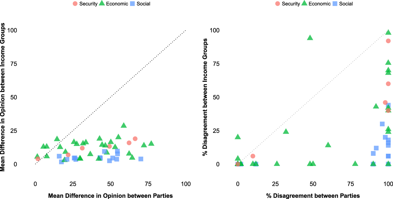
FIGURE 2. Opinion Differences by Issue among Partisan and Income Groups
We plot the mean difference in opinion between Democrats and Republicans against the difference in opinion between rich and poor voters (left) and the percentage disagreement between Democrats and Republicans against the percentage disagreement between rich and poor voters (right). The 45° line is shown.
How often do different segments of the public share the same policy preference? Table 1 displays opinion agreement rates between various subgroup medians. Democratic opinion coincides with the statewide median more than does Republican opinion; poor and rich agree with the statewide median at roughly equal rates. Importantly, Republican copartisans agree with the rich more often than with the poor, while Democrats agree with the poor more than the rich. The subgroup of those we study least reflective of the median voter is the rich Republicans. The subgroup most reflective would be independents, followed closely by the rich.
TABLE 1. Opinion Agreement between (Sub)Group Medians (%)

Standard errors around these given uncertainty are approximately one percentage point.
Party conflict is high and pervasive. Democratic and Republican medians only agree 38% of the time. If we look further, at rich and poor quantiles within each party by state, poor Democrats and poor Republicans only agree 42% of the time (not shown). Rich Democrats and rich Republicans only agree 30% of the time. Indeed, rich Democrats are more likely to agree with poor Republicans (41%) than with the rich ones. Rich Republicans are more likely to agree with the overall poor (44%) than with the Democratic rich. Within parties, there is much more agreement. Rich and poor Democrats agree 89% of the time and Republicans 84%.
RESPONSIVENESS
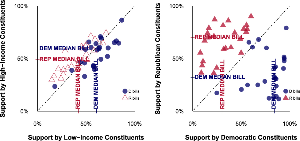
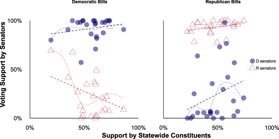
Using these data, Figure 3 shows slopes for responsiveness to poor, rich, statewide, and copartisan opinion first for all senators, and then broken down by party. For all senators, the slope is steeper for rich than poor (as in Gilens), but steeper still for copartisans. Democrats seem strongly responsive to the preferences of all four normal categories of opinion (omitting the opposing partisan group). Republican voting behavior seems anti-responsive to every group, except copartisans.
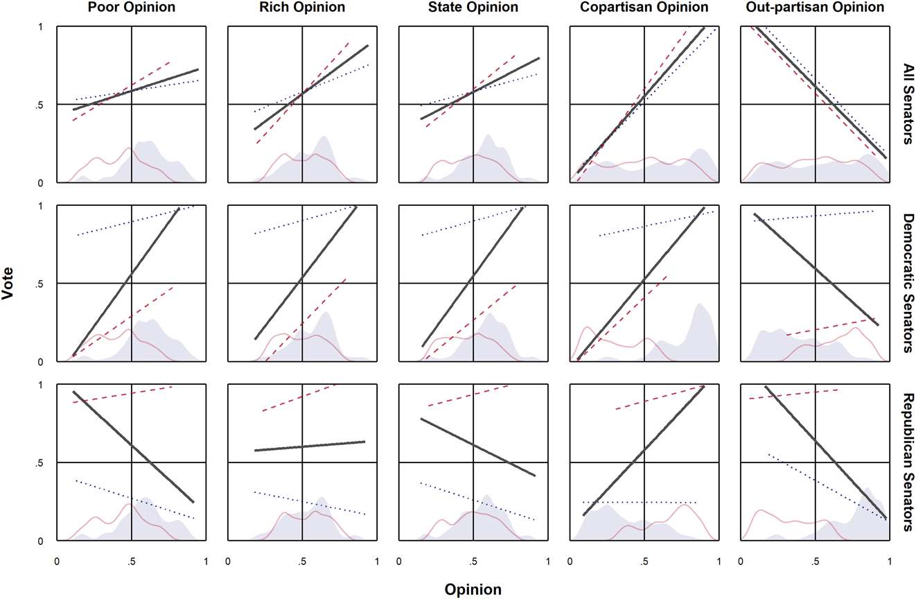
FIGURE 3. Support for Each Party’s Bills among Constituent Subgroups
We show responsiveness for all senators (top row), Democrats (middle), and Republicans (bottom). Outlined and shaded density curves on the x-axis show the distributions of opinion for Republican and Democratic bills respectively. Linear regression lines show responsiveness to subgroup opinion (thick lines for all bills, and dotted or dashed for Democratic and Republican bills respectively.
Are Republicans actually responding perversely to public opinion? Sometimes, but it is not so simple. Note that the average Democratic bill is more popular,Footnote 19 which can be seen in popularity distributions along the rug of Figure 3 or more directly in Figure 4, at the level of the bill.

FIGURE 4. Responsiveness
Figure 5 breaks down responsiveness by the partisanship of the bill. The party difference in voting on bills—the striking intercept shift—is important. Republicans vote against bills the Democrats side with, and Democratic bills are more popular, leading to their appearing anti-responsive overall (this too can be a Simpson’s paradox). On top of that, Republicans are indeed anti-responsive within the set of Democratic bills. By contrast, the Democrats are more responsive to opinion on bills, both their own and those led by the other party. Republicans are mildly responsive to opinion on their own bills. This result is consistent with existing work that finds partisan differences in responsiveness to public opinion (Clinton Reference Clinton2006; Warshaw Reference Warshaw2012; Krimmel, Lax, and Phillips Reference Krimmel, Lax and Phillips2016), a pattern that will repeat itself in our congruence analysis.

FIGURE 5. Responsiveness by Bill
In Table 2, we build from the bivariate analyses (as shown in Figure 3) to multivariate analyses of responsiveness, allowing for varying slopes and intercepts. The first panel presents results for all senators, the second for Democrats, and the third for Republicans. Within each, there are three bivariate regressions of senator’s roll call vote on rich or poor or copartisan opinion, three multivariate regressions each including two of the three aforementioned, and a final regression with all three. Perhaps more than anything else, the results show how difficult it can be, as in Gilens’s data, to tease out different effects using responsiveness regressions alone. Overall, public opinion is a robust predictor of roll call voting, but there are differences in coefficient sizes across subgroups and by senator party. In the models that include all three preference measures, it is the coefficients on rich and copartisan opinion that are largest and most consistently statistically significant. Among Democratic senators, the difference in coefficients on rich and poor opinion is smaller than that among Republican senators. (To give a sense of scale, a coefficient on opinion of 0.16 corresponds to up to a four-percentage-point increase in the probability of a yes vote, for a senator on the tipping point between yes and no.)
TABLE 2. Regressions of Vote on Subgroup Support

Bayesian logit models, using BLGMER in R. Standard errors beneath the coefficient.
Models include random intercepts and slopes for the opinion values by issue.
Opinion (using point predictions) is centered and scaled so that a one unit change is one percentage point.
Better penalized fit for a given data subset is shown by lower AIC. Percent correctly predicted (PCP) is shown.
Table 3 is parallel to the previous table, but regresses vote on the dichotomous position of the median of the relevant subgroup instead of the actual opinion level. This takes a step in the direction of our taking sides analyses. Public opinion, of course, remains a robust predictor of roll call voting. In this table, however, it is the coefficient on partisan opinion, in the form of the partisan median, that consistently has the largest coefficient (e.g., in model 7, a coefficient around 4 is a full swing in probability of a yes vote). Once again, among Democratic senators, the difference in the estimated coefficient on rich and poor opinion is smaller than among that Republican senators.
TABLE 3. Regressions of Vote on Subgroup Opinion Median Position

Bayesian logit models, using BLGMER in R. Standard errors beneath the coefficient.
Models include random intercepts for the opinion dummy variables by issue.
Point predictions for opinion are used.
AIC and PCP are shown.
Collectively, these regressions, although messy to interpret,Footnote 20 do provide some further evidence that there are partisan differences in responsiveness to the opinions of poor constituents and that the opinions of copartisans have an meaningful and independent impact on roll call voting.
However, given problems of collinearity, we need to be careful not to place too much faith in these regressions. And, as we noted above, “Responsiveness-Congruence Independence” means that responsiveness can coexist with biased representation, without congruence, and thus with a significant democratic deficit. Thus, one must await congruence and “taking sides” analyses to get a full picture of representation. We also need to know how the odd anti-responsiveness above (among Republicans) translates into congruence, as well as how the multiple opinion influences found in the regressions translate into bottom-line representation.
CONGRUENCE
We next consider congruence, that is, whether the subgroup median actually gets the vote that it desires from its senator. We first report congruence by subgroup and then contrast across groups. Figure 6 plots congruence rates with uncertainty, with values shown in Table 4.
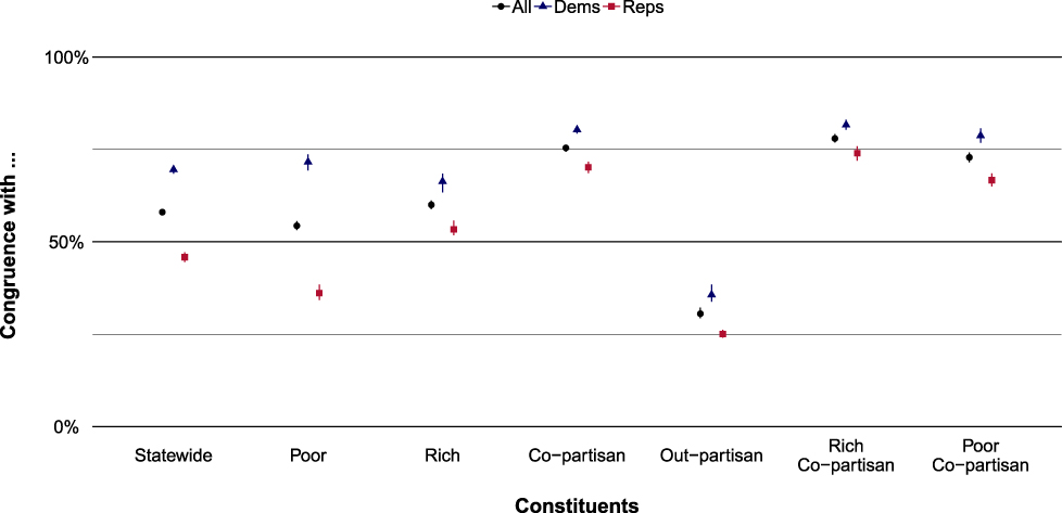
FIGURE 6. Congruence of Senators’ Votes (%), with Uncertainty
A 99% confidence interval represents uncertainty around congruence estimates.
TABLE 4. Congruence of Senators’ Votes (%)

Congruence averaged across all roll votes is a meager 58%. In general, the rich do a bit better than the poor, with a five-percentage-point advantage. However, this advantage is notably smaller than that enjoyed by copartisan constituents who see a congruence rate 16 points higher than that of the rich. Indeed, even poor copartisans enjoy a rate of congruence that is 13 points greater than the rich (although among copartisans, the affluent do slightly better than the poor).
Once again, we see that Democratic senators appear to be more responsive to public opinion than their Republican counterparts. Democrats more frequently cast votes consistent with the preferences of state medians, rich medians, poor medians, and copartisan medians than do Republicans. Democrats are even more likely to vote in line with the rich than are Republicans, but vote more in line with the poor than the rich. Republicans vote more with the rich than the poor.
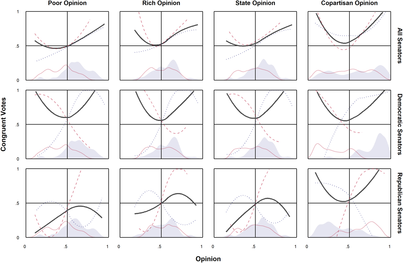
Next, Figure 7 is similar to Figure 3 but with the y-axis capturing congruence with majority opinion instead of a yes vote. A steep U-shape would show strong majoritarian responsiveness, with a softer shape the more likely pattern of weak responsiveness to bare majorities and congruence at the strong extremes. Again, we look at congruence with the various subgroups. Overall, the patterns look normal, lumping all senators together… or taking just the Democrats. The Republicans look, if anything, anti-congruent. The larger the opinion supermajority, the more clear-cut the majoritarian position, the more likely the Democratic senators are to side with it and Republicans against it. Again, break this down further to see why this is the case. The dotted lines show votes on Democratic bills and the dashed lines on Republican bills. Republicans vote for unpopular Republican bills (as Republican bills are typically during this time period) and against popular Democratic bills (as Democratic bills were in this time period). The Democrats meanwhile voted more often for the bills of their own party (which were popular) and against those of the other (which were not). Again, different levels of aggregation can reveal different patterns, for congruence as well as responsiveness. And the degree to which the partisan orientation of a bill drives what happens is both striking and dangerous to ignore, even for evaluating congruence by class.

FIGURE 7. Congruence
We show congruence curves for all senators (the top row), Democrats (middle), and Republicans (bottom). The relative distribution of opinion is shown along the x-axis. The outlined and shaded density curves show the distributions of levels of public opinion. Locally weighted regression lines show responsiveness to poor, to rich, to statewide, to copartisan, and to opposing party opinion. The black lines cover all issues; the dotted and dashed lines cover Democratic and Republican bills, respectively.
We now shift to the senator as unit of analysis, to compare degrees of congruence across subgroups. Figure 8’s top left panel plots each senator by degree of congruence with low- and high-income constituents, whether or not they agree with each other (unlike “taking sides” to come).
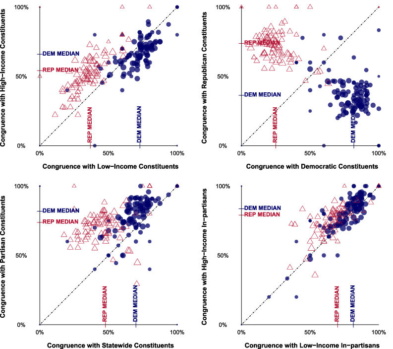
FIGURE 8. Congruence of Votes with Opinion Groups by Senator: Class, Partisan, and State
Each panel shows congruence rates for Democratic (circles) and Republican (triangles) senators for two types of constituent opinion, symbols scaled to the number of votes.
Democrats vote on average with public opinion of both groups more than do the Republicans. That is, both rich and poor are more likely to see their preferences converted into actual senate votes by the Democrats. The Republicans tend to be above the 45° line and the Democrats below, showing their respective tilts toward rich and poor, even given the Democrats higher congruence to both rich and poor. The top right panel compares congruence rates with partisan medians, showing the expected pattern. The bottom left panel shows congruence rates with partisan medians versus statewide medians. Once again, Democrats have not only higher congruence rates with statewide medians but also (slightly) better satisfy their own partisan medians. Finally, the bottom right panel shows congruence with in-party rich and poor. Democrats here too show higher congruence on both dimensions, with both parties roughly along the 45° line.
What we have learned? What do we still need to know? Congruence thus far has not been zero-sum—rich and poor medians often agree, as do party medians and class medians. Recall from Table 4 that the rich saw congruence only five points higher than the poor (60 to 55). Differences in congruence rates are not large, but there are already striking partisan patterns. The Democrats are the party of higher congruence, yet tilt a bit toward the poor. The Republicans are less congruent in their votes than a random coin flip, except (barely) with the rich. Copartisan congruence is quite high, making it all the more important to let copartisans and the rich go head to head. What happens when they clash and a senator must take sides?
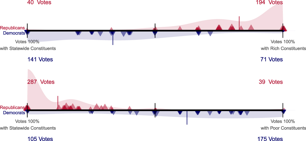
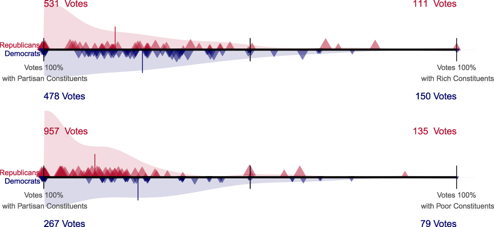
TAKING SIDES
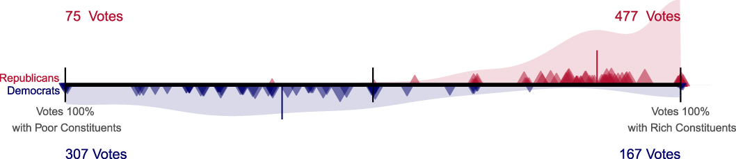
We begin with instances where there is conflict between the opinions of a senator’s rich and poor constituents. Senators side with the rich against the poor 63% of the 1,026 relevant votes. So far, this is similar to Gilens. The parties, however, are quite different on this point: Democrats side with the rich on only 35% of 474 votes, while Republicans do so on 86% of 552 votes.Footnote 21
We explore this type of zero-sum taking-sides conflict in a series of figures, starting with Figure 9. Each panel limits the set of votes to where a particular conflict exists, between one set of constituents on the left and another on the right. Each triangle plotted is a senator’s “score,” the percentage summarizing how often they voted for one side or the other, ranging from 100% left (0% right) to 50–50 to 100% right (0% left). Triangle sizes are scaled to the number of votes by senator. Democrats and Republicans are separated below and above the line, respectively. We can see how senators vary by party by the shaded Gaussian density distributions. We also show the number of votes that fall into the categories.

FIGURE 9. Taking Sides—Class Conflict
Figure 9 continues exploring the results discussed above. The median Democrat tilts toward the poor with 65%. However, there is a fair amount of variation among Democrats. For example, Sen. Russ Feingold is among those on the far left, siding with the rich against the poor in only one of nine votes, while Sen. Claire McCaskill did so in four of six votes. Republicans far more strongly side with the rich; their median senator in this subset did so 91% of the time. The overall level of pro-rich bias is being driven by Republican senators, most strongly by senators such as Sen. James Inhofe with all eleven of his votes, or Sen. Olympia Snowe with six of nine.Footnote 22 These results are consistent with findings that Republicans are more responsive to the wealthy than are Democrats (cf., Bartels Reference Bartels2008; Ellis Reference Ellis2017; Rhodes and Schafner Reference Rhodes and Schaffner2017).
Figure 10 brings in statewide median constituents. The median Democratic senator in the top panel sides with the statewide median more than the rich, and the median Democrat in the bottom panel sides with the poor over the statewide median (again with variation among Democrats). Republicans strongly align with rich over statewide and with statewide over poor.

FIGURE 10. Taking Sides—The Median Voter
Figure 11 shows the expected partisan split for context—when the party medians disagree, senators strongly but not monolithically favor the position of copartisans. Many senators cross the aisle. A handful of “mavericks” are more likely to represent out-partisans than in-partisans: Democrats Zell Miller and Bob Torricelli; and Republicans Olympia Snowe, Susan Collins, Arlen Specter, and especially Lincoln Chafee (but not, surprisingly, John McCain, voting with his party on 22 of 30 such votes). The bottom panel shows senators match copartisan opinion more than their statewide median opinion, showing a clear and strong partisan distortion to representation.
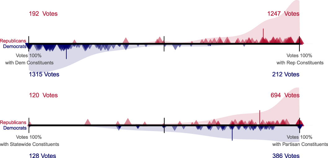
FIGURE 11. Taking Sides—Party Conflict
Figure 12 combines these threads (finally!), with conflict between class and partisanship. The top panel shows that both parties’ senators mostly side with copartisan medians over the rich. The rich median may beat the poor two to one in a direct fight, but the copartisans beat the rich four to one. Both parties also side with copartisans over the poor (bottom panel). In both panels, the Republicans tilt further to partisans than do the Democrats. Republicans who sided with the rich over the party were Snowe, Collins, Specter, and Chafee. The only Democrats who did so (and had more than four such votes pitting the rich against their partisan voter) were Nelson and Carper.

FIGURE 12. Taking Sides—Party or the Purse
We can dig further. Figure 13 shows that what is really pivotal is where the party median stands, alongside the rich median or instead the poor one. The poor win when the copartisans are on their side. Of the 51 times a Republican senator faced a Republican median siding with the poor against the rich, the Republican senators cast 38 votes with the former (75%). Democratic senators similarly voted with party and poor over rich 76% of the time. While the Republicans drive the high victory rate of rich medians over poor medians, that in turn depends on Republican constituents aligning with the rich; when they align with the poor, the rich advantage becomes a poor advantage. The rich do a bit better than the poor comparing both panels, but the partisan thumb on the scale is heavy.

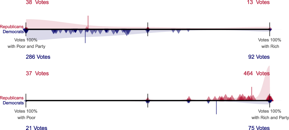
FIGURE 13. Taking Sides—Partisans Take Sides
Another way to consider partisan opinion is to look within copartisan subgroups, at conflict within the partisan constituency. For example, taking the top 20% of Democrats in the state by income, what is the median position? Out of 49 policies by 50 states (2,450 state-policy units), Democratic rich and poor quintiles disagree 11% of the time (on 263 state by issue observations). These areas of intraparty disagreement connected to 267 votes out of the 2,473 cast by Democratic senators that forced a choice between pleasing the in-state Democratic rich and Democratic poor. Republican rich and poor disagree 16% of the time (384 out of 2,450), connecting to 350 votes (out of 2,323 total) that forced a choice for Republican senators.
Here, in this limited set of votes, when there is disagreement between the poor and rich within a party, we do find a pattern of affluent influence not limited to Republicans. Figure 14 shows how senators take sides between copartisan poor and copartisan rich, parallel to the top of Figure 9. Senators side with copartisan rich 72% of the time, with a moderate difference between Republicans (78%) and Democrats (63%).
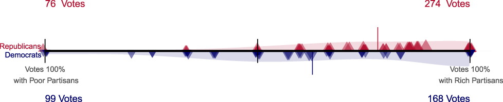
FIGURE 14. Taking Sides—Rich and Poor within Party
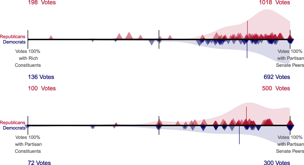
All this so far has set aside yet another aspect of partisanship, the elite party line. Figure 15 explores this dimension of partisanship: how does a senator vote when the modal position of her copartisan Senate peers conflicts with that of her constituents? We do not see pure party-line voting, but the party position trumps that of rich and of the partisan nonelite over 80% of the time in both parties. Those Republicans who broke from their fellow partisans and aligned (coincidentally or not) with the rich were the usual suspects: Sens. Chafee, Collins, Snowe, and Specter. Whatever pull the rich have (or partisan constituents have, for that matter), the party line beats it most of the time, even for Republicans. This reveals a sharp limit to affluent influence and responsiveness in general. Always voting the party line, as formed by Senate partisan coalitions, would only yield 56% congruence (observed level 58%).

FIGURE 15. Taking Sides—Partisan Senate Peers
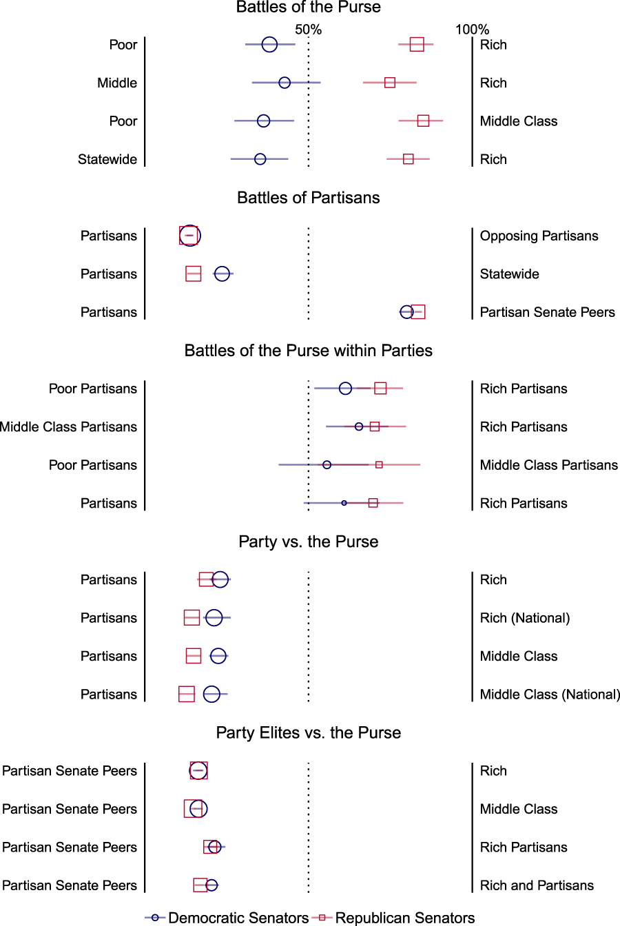
Taking this narrative as a whole, how well-off are the rich? Figure 16 summarizes, simplifies, and adds further information, by incorporating the uncertainty in our congruence estimates.

FIGURE 16. Taking Sides Summary
Summary percentages of voting with conflicting groups. Point predictions, based on median across simulated draws, for the Democratic percentage are the hollow circles and Republicans hollow squares. Point size reflects the number of votes. 99% confidence intervals are shown.
This figure also shows what happens when middle income constituents conflict with others: rich versus middle looks like a slightly attenuated version of rich versus poor and both are similar to middle versus poor (i.e., the same partisan pattern). Throughout, comparisons involving the middle tell the same story as our series of taking sides graphs suggest.
Figure A.5 (in the Online Appendix) shows we get the same “taking sides” results if we limit votes to where the opinion levels are divided by at least 10 percentage points, or where opinion levels are not within five points of the 50% majoritarian cutoff, or where the state Senate delegation is split with one Democrat and one Republican. These robustness checks show the 50% cutoff is not driving our findings.
The pattern in Figure 16, capturing our main inquiry, is clear. Yes, the rich get what they want more often than the poor… when the partisans and the rich agree. Partisanship conditions and constrains class clout. The rich largely have Republican partisanship to thank for any greater influence they have.
There are two ways the rich benefit from Republicans. First and foremost, Republican constituent medians tend to side with the rich more than with the poor. Second, and secondarily, when class differences exist within the Republican constituent coalition, Republican senators side with the Republican rich over the Republican poor. In this latter sense, so do the Democrats side with their own partisan rich over their partisan poor, albeit to a less distorting degree. Rich partisans beat out middle-class partisans and the latter beat poor partisans.
One should be careful not to overstate the substantive impact of Republican senators’ tendency toward the rich. There are only four Republican pro-rich votes (out of 2,323 Republican votes total) that oppose both the statewide median and copartisan median (in these same four, they also oppose the poor median and the median partisan peer).
DISCUSSION AND CONCLUSION
Our analysis of Senate roll call voting brings together, for the first time in a quantitative empirical inquiry, constituent opinion by income and party. Doing so allows us to evaluate, in tandem, class and partisan distortions to representation, to gain a more complete understanding of each, and to document the ways in which they interact. Erikson (Reference Erikson2015, 24) described the affluent influence argument as a “consistent narrative that political representation may be a luxury available to the wealthy alone.” We instead find that the partisan distortion dominates—party beats the purse.
While the affluent dominance model is descriptively correct—in that the rich do get what they want more often than the median voter or the poor—this seems as coincidental as the oft-dismissed coincidental representation of the poor. Combining the relatively moderate pro-poor Democratic bias and the larger pro-rich bias of the Republicans, the result is a party system that over the last two decades favors the affluent, as a result of the outcomes of partisan conflict. Republican partisanship is the key to understanding modern affluent influence. The one exception is a quite limited set of conflicts within party: both Democrats and Republicans side with their rich copartisans over poor copartisans.
If the rich are rigging the system, as some suggest, it would have to be through elections (electing Republicans who cater to Republican voters who more often agree with rich than poor), through convincing Republican voters to favor the policies the rich like,Footnote 23 through taking advantage of redistricting rules to advantage Republicans, and/or through agenda control (since we study only votes that take place, not those that could). We do not address such pathways. At least when it comes to one important pathway—how senators vote—we find the rigged system claim overstated.
In fact, if the rich did control how senators vote—if every senator voted in line with his or her state’s rich median, then instead of only the observed 58% congruence rate overall, we would observe a whopping 91%. (If majoritarian representation is the standard, affluent influence would actually help.) If the poor dominated, congruence would be 87%. If copartisan medians dominated, congruence would be 72%. Listening to public opinion of even such subgroups would be much more majoritarian than the status quo.
Even this obscures party differences, in that if every senator voted the Democratic party line (i.e., in line with the median Democratic senator), congruence would be 67%. It would only be 36% if every senator followed the Republican party line. The poor would be better represented in policymaking if Democrats won more often, in that poor medians would get what they want more often… but so too would the rich, middle, and statewide medians. If Democrats consistently controlled the levers of power (in this time period), one would likely find little (although not necessarily no) evidence of affluent influence. Affluent influence that results from partisan influence may be worrisome, but it is not the same as living in an oligarchy.
Obviously, there remain unanswered questions that are ripe for future investigation. Building upon efforts by Ellis (Reference Ellis2017) and our results here, one could consider why some senators’ roll call voting patterns exhibit a greater bias toward copartisan or elite opinion than others (and our “taking sides” graphs clearly show that there is intriguing variation to be explained). Such an analysis might explore electoral competitiveness, the extent of state-level economic inequality, or union strength. It might also consider senator political ideology or wealth. While we generally focus on differences in responsiveness across senators aggregated at the party level (finding, inter alia, Democrats to be more responsive), a next step might look at variation across individual legislators.
We hope that our detailed prescription for a particular approach to studying these issues and our detailed implementation of this approach will influence other such work in both theoretical approach and empirical detail, building on it—or challenging it—to collectively do our best to untangle these thorny issues.
SUPPLEMENTARY MATERIAL
To view supplementary material for this article, please visit https://doi.org/10.1017/S0003055419000315.
Replication materials can be found on Dataverse at: https://doi.org/10.7910/DVN/MCWFCS.
APPENDIX: THE LUMPING-SPLITTING PARADOX
Consider three senators, from conservative state C, liberal state L, and moderate state M, defined by average opinion across issues, along with three liberal policies to vote on. Figure 17 regresses a liberal policy index (count of liberal policies supported) against a liberal opinion index (average opinion) to yield see a reassuring positive responsiveness slope.

FIGURE 17. Lumping Three Policies (from Table 5)
The opinion levels and votes behind these lumpy averages are shown in Table 5.
TABLE 5. Splitting the Lump

What happens when we split the lump?
Figure 18 shows “splitty” responsiveness. For each policy, responsiveness is actually perverse, with more liberal opinion “causing” a lower chance of the liberal policy. It is not that we expect such anti-responsiveness, but rather that even perverse split responsiveness is compatible with the appearance of lumpy responsiveness. Lumpy responsiveness is not sufficient for split responsiveness.

FIGURE 18. Splitting the Lump (from Table 5)
Next, consider a different set of three policies and opinion levels, graphing responsiveness with a splitting approach in Figure 19.

FIGURE 19. Splitting Three Policies (from Table 6)
Each split responsiveness curve looks normal: higher liberal opinion positively associates with having the liberal policy. Table 6 shows opinion and policy details, and Figure 20 graphs lumpy responsiveness.
TABLE 6. Splitting


FIGURE 20. Lumping the Split (from Table 6)
Now, we find the appearance of perverse lumpy responsiveness. Lumpy responsiveness is thus neither sufficient nor necessary for true responsiveness.


Comments
No Comments have been published for this article.