2.1 Model of the first stage of the spacecraft

In estimating the takeoff-mass of the two-stage spacecraft, the following simplified dynamic model in the vertical plane is used^{(Reference Ruan and Lv6)}.

(1) \begin{equation} \begin{cases} {\frac{dV}{dt} =\frac{F\cos \alpha\,-\,D\,-\,mg\sin \theta }{m} }\\[10pt] {\frac{d\theta }{dt} =\frac{F\sin \alpha\,+\, L\,-\,mg\cos \theta }{mv} }\\[10pt] {\frac{dx}{dt} =V\cos \theta } \\[10pt] {\frac{dh}{dt} =V\sin \theta } \\[10pt] {\frac{dm}{dt} =-\dot{m}}\\[10pt] {u_{1} =\dot{m}}\\ {u_{2} =\alpha =\vartheta -\theta } \end{cases}\label{eq1} \end{equation}

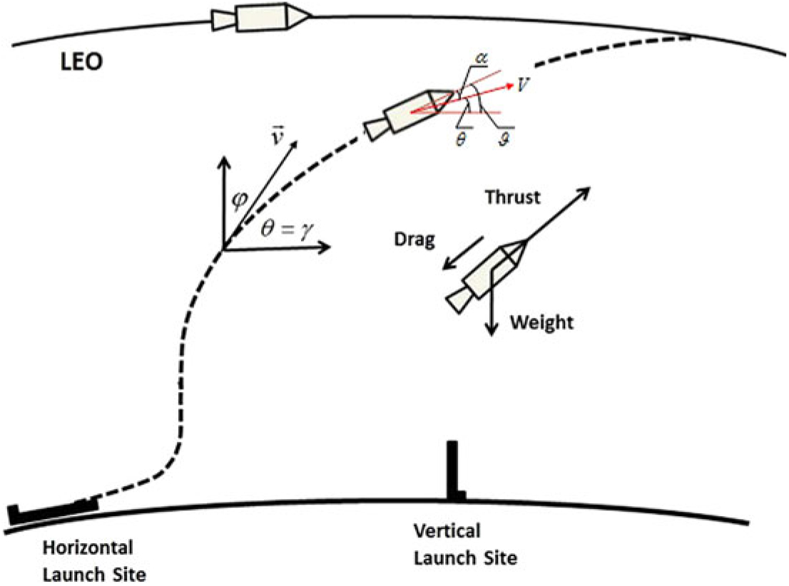
where u ₁ and u ₂ are two control variables. The illustration of the flight trajectory and critical mission altitudes is depicted in Fig. 3^{(Reference Daidzic17)}.

Figure 3. Spaceplane GT (α = ϑ–θ) trajectory when launched nearly horizontally. Not to scale.

The thrust and aerodynamic forces are as follows:

(2) $${\rm{ }}\left\{ {\begin{array}{*{20}{c}} {F = \dot m{I_{sp}}{g_0}} \\ {D = {C_d}Q{S_r}} \\ {L = {C_l}Q{S_r}} \\ \end{array}} \right.$$

C _d and C _l are shown in Tables 1 and 2^{(Reference Brock and Captain18)}; I _sp is shown in Tables 3–5^{(Reference Meyer, Chato, Plachta, Zimmerli, Barsi, Van Dresar and Moder16)} under ejector mode, ramjet mode and scramjet mode, respectively. Tables 3 and 4 are obtained from Ref. 19 and Table 5 from Ref. 20. The aerodynamic raw data of the first-stage aircraft is obtained from the X–43A^{(Reference Brock and Captain18)}. The aerodynamic raw data of the second-stage aero-vehicle is computed by using the Missile DATCOM^{(Reference Ruan, He and Lv21)} software. Q = ρV ²/2 is the dynamic pressure and is assumed that Q Q ≤ Q _max under the ejector mode, Q = Q _maxunder the ramjet and scramjet mode, (where Q _max is the maximum value of dynamic pressure Q); ρ is calculated as follows:

(3) $$\left\{ {\begin{array}{*{20}{c}} {\rho = 1.225{{\left( {1 - 0.000022557h} \right)}^{4.255886}},\quad \quad h \le 11000} \hfill \\ {\rho = 0.36391{e^{ - 0.000157688\left( {h - 11000} \right)}},\quad \quad 11000 \lt h \le 20000} \hfill \\ {\rho = 0.088035\left( {1 + \frac{{0.001\left( {h - 20000} \right)}}{{216.65}}} \right),\quad \quad h > 20000} \hfill \\ \end{array}} \right.$$

Table 1 Drag coefficient C _d

Table 2 Lift coefficient C _l

Table 3 I _sp of ejector mode

Table 4 I _sp of ramjet mode

Table 5 I _sp of scramjet mode

2.2 Calculation of thrust

The takeoff-mass m ₀ of the two-stage-to-orbit spacecraft includes the first stage of launch vehicle mass m ₀₁, and the second-stage RKT rocket mass m ₀₂ includes the payload. m ₀₁ includes the fuel mass, m _01p, and the fuselage structure mass, m _01s^{(Reference Etele, Hasegawa and Ueda5)}, namely,

(4) \begin{equation} m_{0} =m_{01} +m_{02} =\left(m_{01p} +m_{01s} \right)+m_{02}\end{equation}

Thus, we can get the inert mass fraction η of the first-stage RBCC spacecraft

(5) \begin{equation} \eta =\frac{m_{01s} }{m_{01p} +m_{01s} }\end{equation}

The RBCC engine is the first-stage propulsion system, and the liquid rocket engine is the second propulsion system. There are two calculation condition assumptions^{(Reference Ruan, He and Lv21)}:

1. 1. The liquid rocket can shut down or restart according to the requirement. The vacuum specific impulse I _spυ2 is a constant value that does not vary with the flight state. The propellant mass flow rate ṁ is automatically adjusted within a certain range with the thrust requirements.

   2. The RBCC engine works in three modes: the ejector mode (Ma = 0 ~ 2.5), the ramjet mode (Ma = 2.5 ~ 6) and the scramjet mode (Ma > 6.0). The mode conversion is instantaneous. The specific impulse of the RBCC engine is a function of Mach number and flight altitude, and its change law is known. The propellant mass flow can be adjusted. The regulation law and the engine working mode are different. The specific performance is as follows:

   1. a) The ejector mode, assuming that the mass flow of the initial time is ṁ ₀ mass flow in the ejector mode is the largest. Thus, the mass flow of this mode is a function of Mach number and altitude as^{(Reference Ruan and Lv6)}:

      (6) \begin{equation} \dot{m}=\dot{m}_{0} \beta \left(Ma,h\right)\end{equation}

      where 0 ≤ β (Ma, h) ≤ 1, which is subject to the Mach number and altitude and represents the change of ṁ. It can be calculated according to the engine data in the ejector mode and the curve of specific impulse in the Ref. 22. According to the Ref. 21, its calculation method is: if the thrust and specific impulse are known, the engine propellant mass flow rate of a different flight speed and flight altitude can be obtained by the thrust equationF = ṁ I _spg ₀. If divided by the propellant mass flow rate of zero altitude and zero Mach, respectively, then we will get β.

   2. b) The ramjet mode and the scramjet mode

In the ramjet mode and scramjet mode, the ejector rocket will be shut down. The propellant mass flow rate is determined by the amount of air mass flowing into the inlet and the Equivalence ratio Φ,

(7) $$\dot m = \frac{{\Phi \times {{\dot m}_{air}}}}{{\left( {A/{F_{st}}} \right)}}$$

where ṁ _air can be calculated as follows:

(8) \begin{equation} \dot{m}_{air} =k\frac{p^{*} }{T_{stag} } A_{0} q\left(\lambda _{0} \right)\varphi\end{equation}

Then, according to the thrust equation F = ṁ I _spg ₀, the engine thrust of the RBCC can be represented as:

(9) $$F = \left\{ {\begin{array}{*{20}{c}} {{{\dot m}_0}\beta \left( {Ma,h} \right){I_{sp}},\quad \quad 0 \le Ma \le 2.5} \hfill \\ {\frac{\Phi }{{\left( {A/{F_{st}}} \right)}}k{\textstyle{{p*} \over {{T_{stag}}}}}{A_0}q\left( {{\lambda _0}} \right)\varphi {I_{sp}},\;2.5 \le Ma \le 10} \hfill \\ \end{array}} \right.$$

Under certain flight conditions, the engine specific impulse is known. The engine thrust is determined only by the propellant mass flow rate. In the ejector mode, thus, the thrust is determined by propellant mass flow ṁ ₀ at zero time and zero altitude. But in the ramjet mode and scramjet mode, it is determined by the Equivalence ratio Φ, the geometric projection area of air inlet A ₀ and the inlet flow coefficient φ. ṁ ₀ is a given value, A ₀ a constant value and φ a function of Mach number Ma.

2.3 Takeoff-mass constraints of the second-stage liquid rocket

The takeoff-mass of the second-stage liquid rocket can be estimated by the following method^{(Reference Ruan and Lv6)}:

(10) \begin{equation} m_{02} =\frac{m_{pl} }{1-N_{2} -\left(1+k_{2} \right)\mu _{k2} }\end{equation}

and

(11) \begin{equation} N_{2} =N_{2}^{0} +\frac{T_{vac\_ 2} }{R_{T/W\_ 2} m_{02} g_{0} }\end{equation}

(12) \begin{equation} \mu _{k2} =1-e^{\frac{\left(1-k_{2} \right)I_{spv_{2} } }{\Delta v} }\end{equation}

Other coefficients are calculated by the following empirical equations^{(Reference Ruan and Lv6,Reference Ruan, He and Lv21)} :

(13) \begin{equation} \left\{\begin{array}{l} {N_{2}^{0} =0.01\left(1+5e^{-0.034m_{02} } \right)} \\ {T_{vac\_ 2} =m_{02} gT} \\ {\Delta v=v_{orb} -V\left(t_{f} \right)} \end{array}\right.\end{equation}

where

(14) \begin{equation} g=g_{0} \left(\frac{6371000}{6371000+h} \right)^{2}\end{equation}

with g ₀ = 9.80665m/s².

If the thrust-to-weight ratio, the payload of the second-stage rocket, the separation speed and separation altitude are known, we can calculate the takeoff-mass of the second-stage rocket with any given initial value of m ₀₂ through several iterations by using the above method.

3.1 Continuous optimal control problem

For the dynamic system:

(15) \begin{equation} \dot{x}=f\left(x\left(t\right)\!,u\left(t\right)\!,t\right)\end{equation}

where x(t)∊R ⁿ and u(t)∊R ^m are state and control variables, respectively, and the function f:R ⁿ × R ^m × R → R ⁿ determine the control variables to optimize the following cost function:

(16) \begin{equation} J=\Psi (x(t_{f}), t_{f} )+\int _{t_{0} }^{t_{f} }g\, (x(t), u(t), t) dt\end{equation}

and meet the boundary constraints

(17) \begin{equation} \phi\, (x(t_{0} ), t_{0}, x(t_{f} ), t_{f} )=0\end{equation}

and the process constraints

(18) \begin{equation} C\,(x(t), u(t), t_{0} ,t_{f} )\le 0\end{equation}

where ϕ : R ⁿ × R × R ⁿ × R → R ^q and C : R ⁿ → R ^r.

3.2 The basic principle of GPM

The essence of GPM is to replace the original infinite-dimension dynamic optimal control problem with a finite-dimension static nonlinear programming (NLP) by eliminating differential and integral equations. A brief review of pseudo-spectral method (PSM), especially GPM, is presented here. More details can be found in Ref. 12.

Firstly, the original time interval [t ₀, t _f] of the optimization problem is converted to the time interval [−1, 1] as

(19) \begin{equation} \tau =\frac{2t}{t_{f} -t_{0} } -\frac{t_{f} +t_{0} }{t_{f} -t_{0} }\end{equation}

By using Equation (19), Equation (16) is reformulated in terms of τ as:

(20) \begin{equation} J=\Psi (x(1), t_{f} )+\frac{t_{f} -t_{0} }{2} \int _{-1}^{1}g\,(x\,(\tau ), u\,(\tau ), \tau )\, d\tau\end{equation}

Similarly, the dynamic Equation (15) and the boundary constraints (17) are replaced by

(21) \begin{equation} \frac{2}{t_{f} -t_{0} } \frac{dx}{d\tau } =f\left(x\left(\tau \right),u\left(\tau \right),\tau \right)\end{equation}

and

(22) \begin{equation} \phi \left(x\left(-1\right),t_{0} ,x\left(1\right),t_{f} \right)=0\end{equation}

respectively.

In GPM, the Legendre-Gauss (LG) points τ _k (1 ≤ k ≤ N − 1), distributed on the interval [-1, 1], are defined as the roots of

(23) \begin{equation} P_{N} \left(\tau \right)=\frac{1}{2^{N} N!} \frac{d^{N} }{d\tau ^{N} } \left[\left(\tau ^{2} -1\right)^{N} \right]\end{equation}

while τ ₀ = −1, τ _N = 1.

The continuous state and control variables are approximated by the N ^th Lagrange interpolation polynomials in the form

(24) \begin{equation} x\,(\tau )\approx X(\tau )=\sum _{i=0}^{N}L_{i} (\tau)\, X(\tau _{i} )\end{equation}

and

(25) \begin{equation} u(\tau )\approx U(\tau )=\sum _{i=1}^{N}L_{i} (\tau)\, U(\tau _{i} )\end{equation}

where the Lagrange interpolation polynomial is

(26) \begin{equation} L_{i} \left(\tau \right)=\prod _{j=0,\ j\ne i}^{N}\frac{\tau -\tau _{i} }{\tau _{i} -\tau _{j} }\end{equation}

Secondly, the dynamic Equation (15) is discretized at the node points, as in Ref. 15:

(27) \begin{equation} \dot{x}\left(\tau \right)\approx \dot{X}\left(\tau \right)=\sum _{i=0}^{N}\dot{L}_{i} \left(\tau \right)X\left(\tau _{i} \right) \end{equation}

where the differential matrix can be computed offline:

(28) \begin{equation} D_{ki} =\dot{L}_{i} \left(\tau _{k} \right)=\left\{\begin{array}{l} {\dfrac{\left(1+\tau _{k} \right)\,\dot{\!P}_{K} \left(\tau _{k} \right)+P_{K} \left(\tau _{k} \right)}{(\tau _{k} -\tau _{i} )[(1+\tau _{i} )\,\,\dot{\!P}_{K} (\tau _{i} )+P_{K} (\tau _{i} )]} ,i\ne k} \\[12pt] {\dfrac{\left(1+\tau _{i} \right)\,\ddot{\!P}_{K} \left(\tau _{i} \right)+2\,\dot{\!P}_{K} \left(\tau _{i} \right)}{2[(1+\tau _{i} )\,\,\dot{\!P}_{K} (\tau _{i} )+P_{K} (\tau _{i})]},\quad i=k} \end{array}\right.\end{equation}

Thus, the dynamic differential equation constraints are transformed into the algebraic constraints:

(29) \begin{equation} \sum _{i=0}^{K}D_{ki} X\, (\tau _{i}) -\frac{t_{f} -t_{0} }{2}\ f\,(X(\tau _{k} ), U(\tau _{k} ), \tau _{k} ;t_{0} ,t_{f} )=0,\quad k= 1,..., K\end{equation}

Meanwhile the terminal moment node is not included in the approximate expression of state variables. So, the terminal state should satisfy the constraint conditions of dynamic equation, namely,

(30) \begin{equation} x(\tau _{f}) = x(\tau _{0} )+\int _{-1}^{1}f(x(\tau ),u(\tau ),\tau )d\tau\end{equation}

The differential of the terminal constraint and integral can be obtained by Gauss integral, namely,

(31) \begin{equation} X(\tau _{f} )=X\left(\tau _{0} \right)+\frac{t_{f} -t_{0} }{2} \sum \omega _{k}\, f\, (X\, (\tau _{k} ), U\,(\tau _{k} ), \tau ;t_{0} ,t_{f} )\end{equation}

Thirdly, the continuous-time cost function (16) is approximated by Gauss integral, as follows:

(32) \begin{equation} J=\Phi \left(X_{0} ,t_{0} ,X_{f} ,t_{f} \right)+\frac{t_{f} -t_{0} }{2} \sum _{k=1}^{N}\omega _{k} g\left(X_{k} ,U_{k} ,\tau _{k} ;t_{0} ,t_{f} \right)\end{equation}

Similarly, the terminal and process constraints can also be reformulated.

According to the mathematical transformation above, the optimization problem based on GPM can be described as seeking the status variables X _i (i = 0, …, K), the control variables U _k (k = 1, …, K) on discrete nodes and the ending time t _f to minimize the cost function Equation (32). Meanwhile, X _i and U _k satisfy Equations (29), (31) and the following two equations:

boundary constraints

(33) \begin{equation} \varphi \left(X_{0} ,t_{0} ,X_{f} ,t_{f} \right) = 0\end{equation}

and process constraints

(34) \begin{equation} C\left(X_{k} ,U_{k} ,\tau _{k} ;t_{0} ,t_{f} \right)\le 0,\quad k = 1,\ldots ,K\end{equation}

From the procedures described in this section, the optimization problem is transformed into a general NLP, namely,

(35) \begin{equation} \begin{array}{l} {min \quad F\left(y\right)\; \; \; y\in R^{M}} \\ {s.t.\quad g_{j} \left(y\right)\ge 0,\quad j = 1,2,\ldots ,p} \\ \quad\quad{h_{j} \left(y\right) = 0,\quad j = 1,2,\ldots ,l} \end{array}\end{equation}

where y is a designed variable that contains state variables, control variables and the end time.

There are many effective methods to solve NLP availability. Among them, sequential quadratic programming (SQP) is widely used because of its maturity^{(Reference Tawfiqur and Zhou23,Reference Ghorbani and Salarieh24)} .

4.1 Initial values

For the takeoff stage, the rocket must satisfy the initial value requirements, including elevation angle θ ₀, angle-of-attack α ₀, speed V ₀, position (x ₀, y ₀) and mass search interval [m _{0 min}, m _{0 max}]. The optimization objective is to seek the optimal takeoff-mass within the search interval.

4.2 Process constraints

According to the performance specifications of the launch vehicle, the following process constraints should be considered:

(36) \begin{equation} \Phi _{\min } \le \Phi \le \Phi _{\max }\end{equation}

(37) \begin{equation} \theta _{\min } \le \theta \le \theta _{\max }\end{equation}

(38) \begin{equation} Q-Q_{\max } \le 0\; \; \; {\rm the\; ejector\; mode}\end{equation}

(39) \begin{equation} Q-Q_{\max } =0\; \; \; \; {\rm the\; ramjet\; and\; scramjet\; mode}\end{equation}

4.3 Terminal constraints

According to the separation constraint, several requirements of the algorithm should be satisfied with the requirements optimized in their constraint ranges. The following separation terminal constraint ranges are considered: the elevation angle range [θ _{f min}, θ _{f max}], the speed range [V _{f min}, V _{f max}], the position range [x _{f min}, x _{f max}] and [h _{f min}, h _{f max}] and the mass range [m _{f min}, m _{f max}]. Here, f is the terminal time point.

4.4 Control constraints

Here, we select the mass flow ṁ and the angle-of-attack α as the control variables and limit them to

\begin{equation*}{\dot{m}\in \left[\dot{m}_{\min } ,\dot{m}_{\max } \right]}\ {\rm and}\ {\alpha \in \left[\alpha _{\min } ,\alpha _{\max } \right]}.\end{equation*}

4.5 Mass constraint of the second-stage RKT rocket

We investigate the optimal separation time of the RBCC-RKT launch vehicle, and the second RKT rocket is selected as a constraint, which can avoid the double-counting problem and simplify the algorithm (Because GPM is a global optimization algorithm, if the inert mass fraction is taken as a constraint, it can be calculated in the optimization process. If it is not taken as a constraint, it is necessary to find out whether the optimization result meets the inert mass fraction after optimization. If it is not satisfied, it needs to be optimized again, which results in the increase of optimization times.).

The inert mass fraction constraint is

(40) \begin{equation} \frac{m_{01f} -m_{02} }{m_{01} -m_{02} } =\eta\end{equation}

4.6 Cost function

The objective of the optimization is to minimise the consumed propellant mass prior to separation^{(Reference Ruan, He and Lv21)}, but the GPM algorithm seeks the minimum. So, the cost function is then to minimize:

(41) \begin{equation} J_{{1}} =\int _{t_{0} }^{t_{f} }\dot{m} dt\end{equation}

In addition, for the reuse of the rocket, we choose the trajectory inclination angle at separation θ _f = 0 as the cost function as well, namely,

(42) \begin{equation} J_{{2}} ={\rm abs}(\theta _{f} )\end{equation}

For the convenience of solving by GPM, the above three objective functions are summed weighted:

(43) \begin{equation} J=f_{1} \cdot J_{1} +f_{2} \cdot J_{2}\end{equation}

where f ₁, f ₂ are weighting factors.

This multi-objective optimization problem (MOP) of takeoff-mass can be transformed into a general multi-objective parameter optimization problem by using GPM. The Karush-Kuhn-Tucker condition (KKT) of the NLP transformed by GPM is consistent with the first-order optimality condition of the discrete Hamilton boundary value problem under certain conditions^{(Reference Benson, Huntington, Thorvaldsen and RAO26)}. The optimal Pareto front of the multi-objective can be got by using the Normal Boundary Intersection method (NBI) to solve the MOP of GPM^{(Reference Lei, Jianquan, Tao, Zhiwei and Zhengnan27,Reference Logist, Houska, Diehl and Van Impe29)} . For this, the GPM toolbox GPOPS that we used has the following modifications according to the Ref. 27:

1. 1. The Mayer and Lagrange indexes in the cost function are output respectively for each function.

2. 2. The sparse matrix template is modified.

3. 3. The NBI method is added to the GPOPS.

4.7 Aerodynamic data processing

The data in Tables 3–5 of I _sp is segmented, which will cause severe difficulties to the convergence of the optimization process. So, in order to facilitate the use of GPM algorithm, we adopt an integrated interpolation strategy for the data at different stages^{(Reference Chiu30,Reference Pini, Spinelli, Persico and Rebay31)} .

According to the data in Tables 3–5 in different phases, there is no overlap in the Mach dimension so that they can be merged in a straightforward way. To facilitate representation, this composite table is represented as Table I _sp. A specific method is also proposed in the Appendix. Finally, we can obtain a unified rectangular data table, and the data of a two-dimensional curved surface is shown in Fig. 4. A consistent two-dimensional interpolation method can be used to speed-up the convergence of the optimization algorithm.

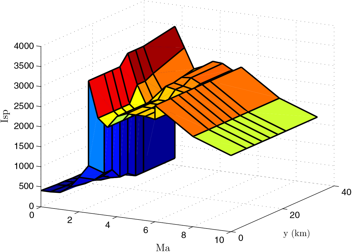
Figure 4. I _sp data.

Air density is a piecewise function of altitude. To make convergence faster, they are also combined in a unified air density table, where the altitude sampling points are [0, 1000, …, 76000](m) with an interval of 1000 m.

4.8 The process to attain the optimized results

Set the number of iterations and the precision requirement, go to Step 1.

1. Step 1: Input the initial value, the precision tolerance and all constraints, where the number of input LG point N is usually a small value at the first time.

2. Step 2: Process the following optimization to obtain the optimal solution by using GPM:

   • min cost function (43)

   • s.t. equality constraints (10)

   • and inequality constraints (36)–(40)

3. Step 3: Solve the NLP with software SNOPT.

4. Step 4: If the iteration number is not reached, and the precision requirement is not met, then increase the number of nodes, N, and go to Step 1. Otherwise, end up with the optimal solution.

5.1 Simulation 1: Flight trajectory before the separation

For comparison convenience, we adopted some values of Ref. 6 and assumed that a two-stage spacecraft takes off horizontally, and the takeoff altitude h = 0km. When the spacecraft takes off from the ground, the elevation angle θ = 0^o, the angle-of-attack α = 7^o, the payload m _pl = 500kg and the Mach number Ma = 0.4. Additionally, Q _max = 105348 Pa, the speed loss coefficient of the second-stage rocket k ₂ = 0.15, the payload injection speed v _orb = 7749m/s and the thrust-to-weight ratio of the second-stage rocket T = 1.2. Then, take η = 0.568, the reference area S _r = 36.144ft ², the vacuum specific impulse of the second-stage liquid rocket I _{spv 2} = 390s, N = 20, precision tolerance = 1e-3. Since the optimal takeoff quality is as important as the successful recovery of the rocket, f ₁ = f ₂ = 0.5 is used to achieve both purposes.

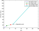
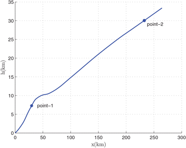
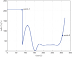
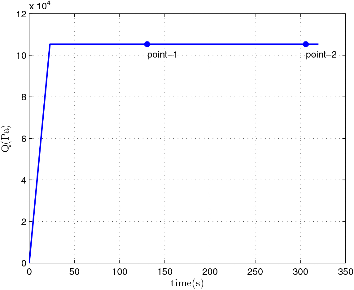
After the optimization, we can obtain the relevant results of the mass of the first-stage rocket m ₀₁ = 38323.5 kg, the mass of propellant consumed prior to separation = 10420.8 kg, the separation Mach number Ma = 7.7414, the separation altitude h = 33528 m, the trajectory inclination angle at separation θ _f = 3.12^o and the takeoff-mass of the second-stage rocket m ₀₂ = 7339.9 kg. Through three main iterations (GPM will sub-iterate itself), when N = 48, the designed optimal result meets the precision tolerance and ultimately reaches convergence, as shown in Table 6. Because of many range constraints, the convergence rate of GPM is slow by using MATLAB, about 704.01s. The optimization results are shown in Figs 5–10. In each figure, there are two points, where point-1 indicates that the ejection mode ends and the ramjet mode starts, and point-2 indicates that the ramjet mode ends, and the scramjet mode starts. Figure 5 shows the angle-of-attack curve, Fig. 6 shows the trajectory curve, Fig. 7 shows the Mach number curve and Fig. 8 shows the propellant flow before the separation. It can be seen that a spacecraft needs to burn more fuel to counteract gravity initially. As the speed increases and atmospheric density decreases, fuel consumption decreases. Figure 9 is the curve of altitude and Mach number, which illustrates that the flight envelope operates within Tables 3–5. Figure 10 is the dynamic pressure, which satisfies the constraint.

Table 6 The convergence history

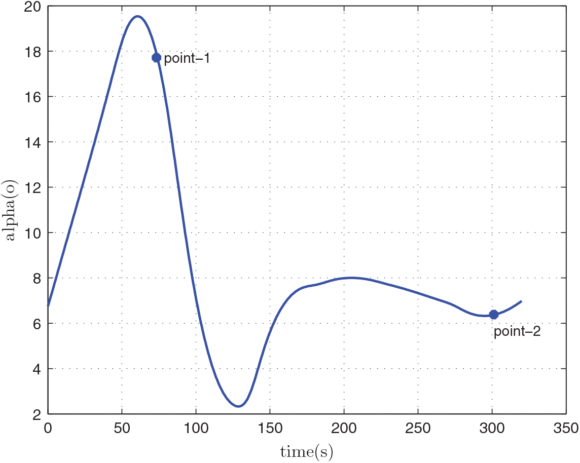
Figure 5. The angle-of-attack.

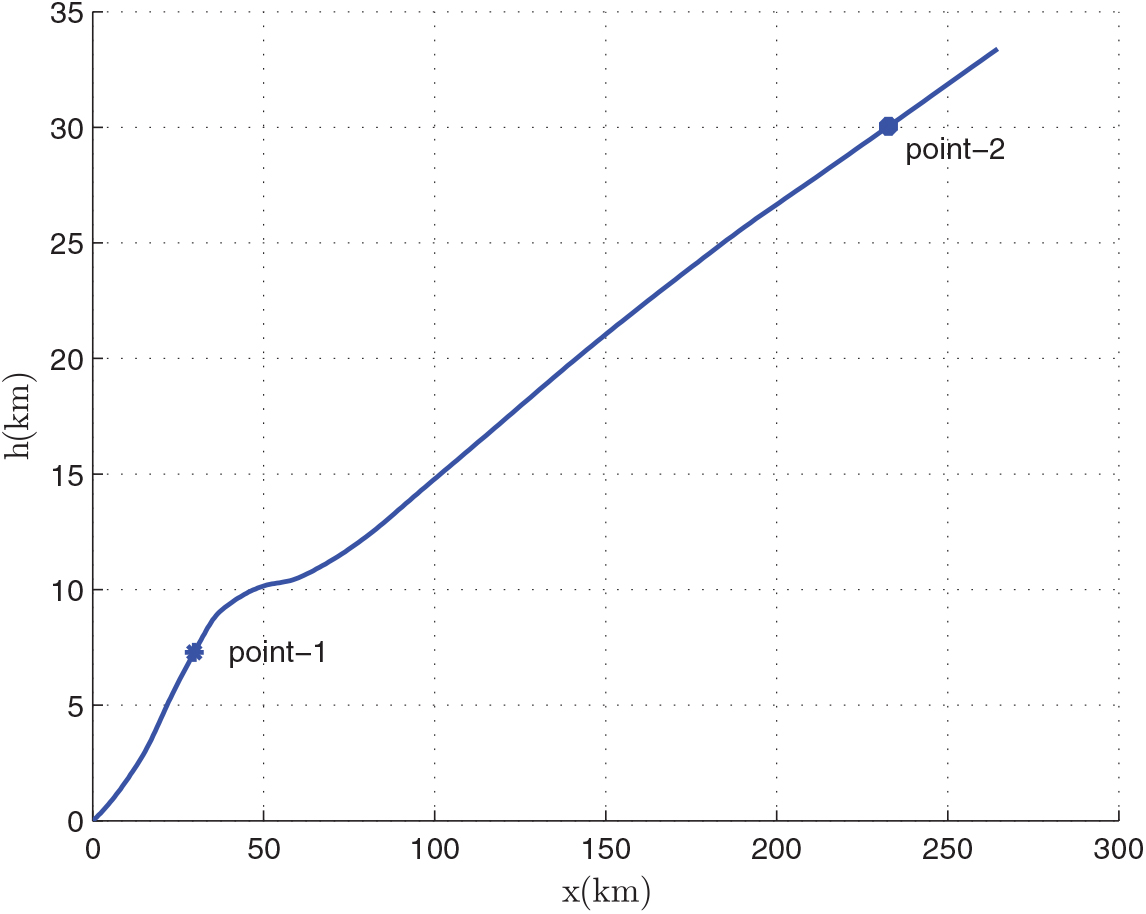
Figure 6. Flight trajectory.

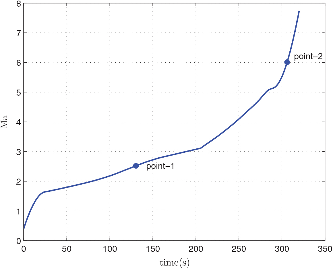
Figure 7. Mach number.

Figure 8. Mass flow rate.

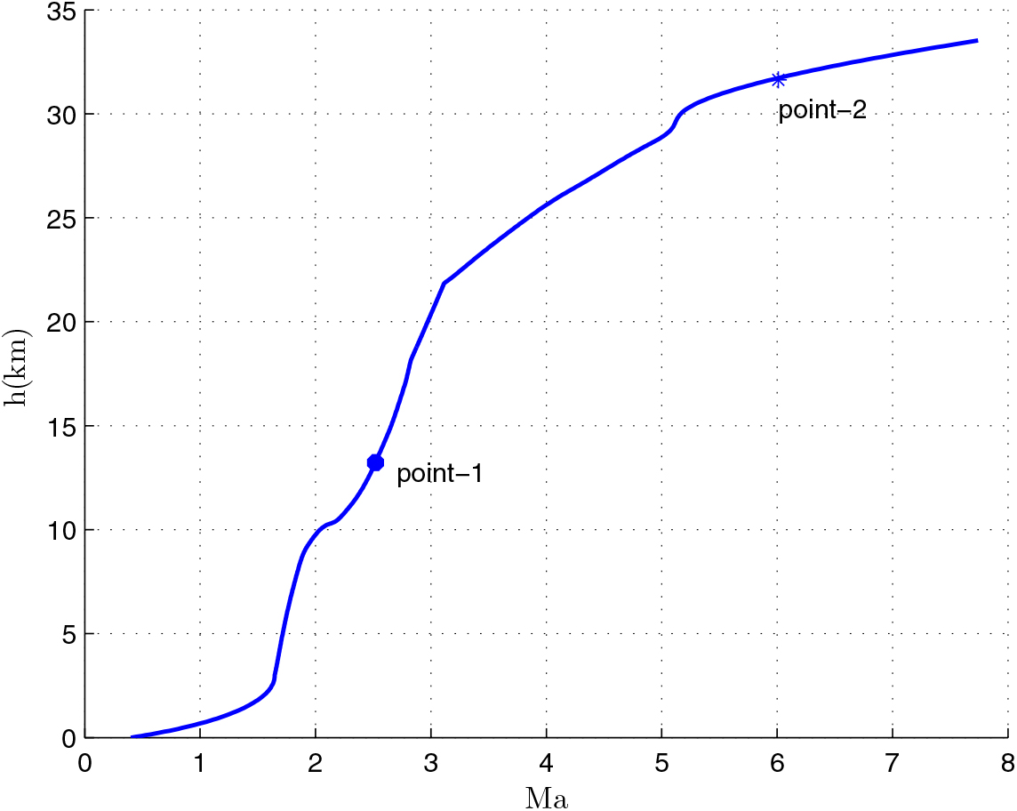
Figure 9. Altitude vs Mach number.

Figure 10. The flight dynamic pressure Q.

We can see that the flight Mach number keeps increasing when the time t < t _f. Furthermore, the Mach number reaches the maximum when t = t _f, and t _f is the optimization end time of GPM optimization process. Thus, t _f is the separation time of the first stage and the separation Mach number is the largest. We can also see that there is a peak and two valley values of angle-of-attack. At the beginning of the flight, angle-of-attack keeps increasing and begins to decrease when reaching a certain value. This is because the initial flight angle is small, and the angle-of-attack must continually increase to raise the trajectory angle of the spacecraft. At the end of the flight, in order to improve the flight speed, the engine thrust of the first-stage rocket needs to increase, but the geometry projection area of the inlet limits the air inflow. So, the angle-of-attack must be reduced. Because of the limitations of the rockets, the angle-of-attack will change again when the rocket reaches its maximum speed.

When the Mach number reaches Ma = 3.5, the rocket enters the flight range of constant dynamic pressure, the engine throttles quickly, the rocket starts to fly along a dynamic pressure path and the engine thrust will be determined by the actual dynamic pressure. From the control process of propellant mass flow rate, we can see that in the ejector mode, the propellant mass of the engine keeps the maximum flow rate at the average of 202. 3 kg/s, and at the average of 51.9kg/s in the ramjet mode and the scramjet mode. So, we can see that the propellant mass consumed is mainly concentrated in the ejector mode.

This global optimal processing of the GPM algorithm is beneficial to reduce the takeoff-mass m ₀₁of the first stage, which has a higher economic value for larger payloads.

5.2 Simulation 2: The relationship of η and m ₀₁

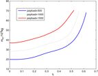
In order to better illustrate the relationship between the first-stage takeoff-mass m ₀₁ and the inertia mass coefficient η with the same payload mass, this paper adopts the cubic spline fitting method to fit the curve of m ₀₁ and η with a different payload mass m _pl, as shown in Fig. 11.

Figure 11. The relationship between payload, η and m ₀₁.

We can see that under certain conditions of the inertial mass coefficient, the larger the payload mass the larger the takeoff mass of the first-stage. This is the same with Ref. 6. However, the average takeoff-mass is smaller, about 530kg. When η is small, m ₀₁ increases a little with the increase of η. When η increases to a certain value, η is the main part of the impact of the takeoff-mass m ₀₁, which will increase rapidly with the increase of η.

In addition, when the takeoff-mass m ₀₁ remains unchanged, the payload mass will decrease with the increase of the inertial mass coefficient η, and the spacecraft will lose its feasibility at the same time. So, for the feasibility of spacecraft, the inertial mass of the spacecraft must be controlled, especially the inertial mass of RBCC propulsion system.

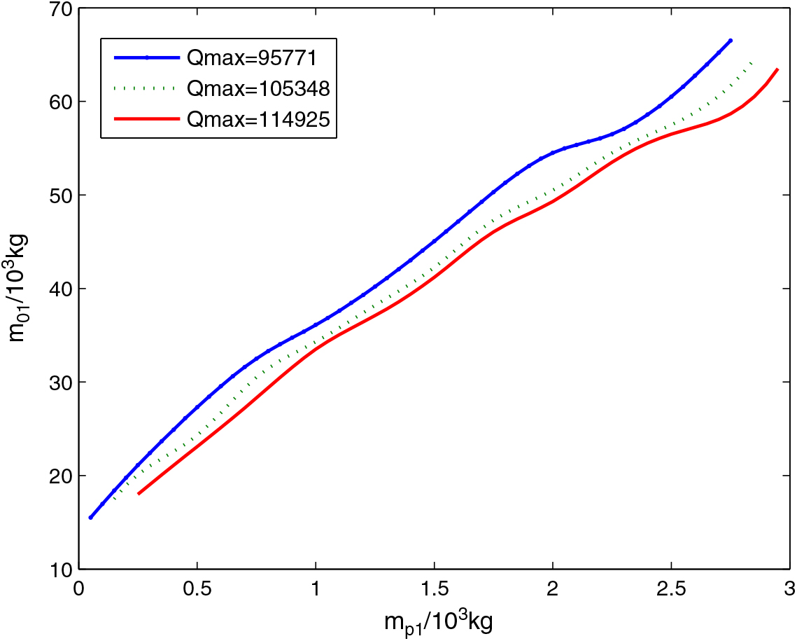
5.3 Simulation 3: The relationship of Q _max and m ₀₁

In order to guarantee that the RBCC engine works steadily in an optimal or stable state, when the spacecraft reaches a certain dynamic pressure, the RBCC-powered spacecraft usually keeps rising and accelerating with a constant dynamic pressure. Namely, the dynamic pressure of spacecraft remains Q = Q _max unchanged in the ramjet mode and scramjet mode. In order to investigate the influence of the dynamic pressure Q _max on m ₀₁, we plot the curves of m _p and m ₀₁ when Q _max= 95771, 105348 and 114925 pa, as shown in Fig. 12. It is clear in Fig. 12 that a higher dynamic pressure maximum Q _max is beneficial to reduce the takeoff-mass of the first-stage. For a RBCC engine, the flight altitude and Mach number, whose relationship is determined by the dynamic pressure, directly affects the inhaled to air inlet mass flow rate and has a greater influence in the ramjet mode and scramjet mode. Because the dynamic pressure maintains a constant maximum Q _max in the two modes.

Figure 12. The relation among Q _max, payload and m ₀₁.

From the point of the engine combustion, RBCC engine prefers a larger dynamic pressure, because under the condition of a certain capture area of air inlet, it can capture more air to increase the engine thrust. However, with the increase of dynamic pressure, the air resistance will increase, and the heat protection requirements of the spacecraft will also be increased.

So, a suitable dynamic pressure is needed for engine control. Appropriate dynamic pressure can throttle the mass flow appropriately. It can also effectively reduce the waste of engine performance caused by the negative angle-of-attack and improve the effective specific impulse. This is similar to the case of Ref. 6, but under the same conditions, our m ₀₁is smaller.