


1. INTRODUCTION
Ship type recognition results provide critical on-site transportation information to maritime traffic participants, including officers of the maritime safety administration (MSA), ships' crews, ship owners and shipping companies. By identifying which ships sailing in coastal channels belong to particular classes of dangerous shipping (e.g., oil tankers, or ships carrying chemicals or liquefied natural gas (LNG)), using maritime closed-circuit television (CCTV) systems, MSA officers can track the positions of dangerous ship in real time, issue early navigation warnings to ships sailing nearby, and thus help relevant traffic participants take early actions to avoid potential maritime accidents. Vessel traffic service (VTS) and automatic identification system (AIS) are the two techniques commonly used for obtaining information on ship type. More specifically, each ship's officer of the watch regularly reports their ship's basic navigation information, consisting of destination port, departure port, ship type etc., to MSA officers via a very-high-frequency telephone (which is a ship-borne VTS facility) once the ship travels into the report line area (Ahn et al., Reference Ahn, Jeong, Endo, Omori and Hashimoto2014). A ship-borne AIS transmitter periodically sends out both static information about the ship (gross tonnage, moulded draft, ship type etc.) and kinematic information to neighbouring ships and inland base stations (which automatically receive the AIS data with AIS receivers) (Silveira et al., Reference Silveira, Teixeira and Soares2013; Sang et al., Reference Sang, Wall, Mao, Yan and Wang2015; Robards et al., Reference Robards, Silber, Adams, Arroyo, Lorenzini, Schwehr and Amos2016; Shu et al., Reference Shu, Daamen, Ligteringen and Hoogendoorn2017). Though the AIS system transmits and receives information on ship type in an automatic manner, the AIS transmitter terminals need to be initialised manually by inputting the information (which cannot be easily erased). Thus, human involvement is essential in the above techniques for obtaining information on ship type. With the rapid increase of volume of maritime traffic and fleet size, these conventional methods become very time-consuming and inefficient in accomplishing the task of ship type recognition.
Researchers have employed techniques based on synthetic aperture radar (SAR) to recognise ship types. Chuang et al. proposed a ship echo recognition framework by applying a novel adaptive detection technique to the original coastal radar images (Chuang et al., Reference Chuang, Chung and Tang2015). Makedonas et al. proposed a two-stage hierarchical feature selection algorithm to discriminate three civilian ship types (i.e., cargo carrier, fisher and tanker) (Makedonas et al., Reference Makedonas, Theoharatos, Tsagaris, Anastasopoulos and Costicoglou2015). Similar research can also be found in Lang et al. (Reference Lang, Zhang, Zhang and Meng2016) and Chen et al. (Reference Chen, Wang, Shi, Wu, Zhao and Fu2019). Zhang et al. (Reference Zhang, Zhang and Zheng2011) proposed a hybrid algorithm, based on cubic b-spline lift wavelet and Canny operator, to extract and recognise ship types. Kaçar et al. proposed a novel approach to classify ship types from synthetic images (Kaçar et al., Reference Kaçar, Kumlu and Kirci2015). It is noticed that both SAR and computer vision based recognition models explored hand-crafted ship features, such as colour, Sobel feature, Canny descriptor etc., for tackling the ship type recognition challenge, however, these features may be contaminated and interfered with by sea clutter interference, resulting in unsatisfactory recognition accuracy (Guo and Ding, Reference Guo and Ding2015).
Deep learning (DL) based methods showed superior performance in tasks of object detection, recognition and classification (Donahue et al., Reference Donahue, Jia, Vinyals, Hoffman, Zhang, Tzeng and Darrell2014; Karpathy et al., Reference Karpathy, Toderici, Shetty, Leung, Sukthankar and Fei-Fei2014; Ferreira and Giraldi, Reference Ferreira and Giraldi2017), and the recognition accuracies of DL based methods were even better than those of humans (He et al., Reference He, Zhang, Ren and Sun2015). The main reason is that DL models were trained with a large number of samples (at different scales, diverse viewpoints, varied lighting conditions etc.), and thus the intrinsic and distinct object features can be efficiently learned and extracted. DL based models are also very popular and efficient in solving maritime challenges, such as ship and iceberg identification (Bentes et al., Reference Bentes, Frost, Velotto and Tings2016), inland ship detection (Lin et al., Reference Lin, Shi and Zou2017), etc.
The success of the DL model in solving maritime problems shows its potential for addressing the challenge of ship type recognition. Convolution neural network (CNN) models, an efficient DL framework, have presented impressive performance in object (i.e., vehicle, traffic signs) recognition tasks in the transportation field (Jin et al., Reference Jin, Fu and Zhang2014; Rainey, Reference Rainey2016; Hu et al., Reference Hu, Zhuo, Zhang and Li2017). For instance, Rainey applied a CNN model to recognise typical merchant ship types from satellite images, and the average recognition accuracy was over 90% (Rainey, Reference Rainey2016). Hu et al. introduced a branch CNN model to reduce the model training time without losing recognition accuracy (Hu et al., Reference Hu, Zhuo, Zhang and Li2017). Jin et al. integrated a hinge loss stochastic gradient descent mechanism into the CNN model, and obtained accuracy of 99·65% when recognising traffic signs (Jin et al., Reference Jin, Fu and Zhang2014).
It is not easy to apply the traditional CNN models to the ship type recognition task, however, for the following reasons. First, ship images may be taken from different viewpoints, and thus the appearance of a ship of the same type may vary significantly, which may mislead the CNN to extract biased ship features for the same ship type. Second, due to limited input training samples, the training process of the CNN model often suffers from over-fitting disadvantage, which leads to a degraded recognition performance. To address the above issues, our research team proposed a novel coarse-to-fine cascaded CNN (CFCCNN) framework for recognising ship types. Considering that the over-fitting phenomenon is mainly caused by lack of training data, the CFCCNN introduces three regularisation methods to extract more universal ship features by different means. We develop a random heuristic selection (RHS) mechanism to select the regularisation model in each fine step in the CFCCNN model, and thus adjust parameter setups to obtain distinct ship features efficiently and accurately.
2. CFCCNN FOR SHIP TYPE RECOGNITION
2.1. Ship type recognition with conventional CNN
CNN based frameworks have shown many successes in the field of object recognition (such as vehicle type identification, image noise type recognition, etc.), being capable of extracting distinct features of objects better than the hand-crafted feature extraction models (Huang et al., Reference Huang, Wu, Sun, Wang and Ding2015; Khaw et al., Reference Khaw, Soon, Chuah and Chow2017; Cao et al., Reference Cao, Gao, Chen and Wang2019). Motivated by the high recognition accuracy of CNN, we proposed to employ the CNN framework to recognise ship types accurately. The standard CNN mainly consists of an input layer, hidden layer and output layer for fulfilling the task, in this case, of ship type recognition (Xu et al., Reference Xu, Lu, Liang, Gao, Zheng, Wang and Yan2016). The feed of the CNN input layer includes the training images of ships, and the corresponding ship labels. The input images involve different types of ships (i.e., the ship types to be recognised) such as oil tanker, container ship, LNG tanker, chemical carrier, general cargo vessel and bulk carrier. The corresponding labels for each input ship type image are also fed into the CNN input layer, which helps the CNN model to mark out different ship types. The input layer of the CNN plays the role of formatting the initial ship images and labels. More specifically, the input layer crops each input ship image to the same size and matches a ship type label to each of the training images. The outputs of the CNN input layer are learnable and trainable ship data, which serves as the training input for the hidden layer.
The hidden layer of the CNN explores the intrinsic features by learning from the previous layers' outputs with the convolution layers, pooling layers and local response normalisation (LRN) layers (see Figure 1). More specifically, the convolution layer explores ship features at different scales, and then the pooling layer is trained to find important scaled ship features (i.e., more distinct ship features). The LRN layer is employed to enhance the generalisation capability of the CNN model. Note that the hidden layer in the CNN nests with the convolution layers, pooling layers and LRN layers, and the outputs of the CNN hidden layer are considered to be the universal ship feature vectors. The output layer of the CNN obtains ship recognition results by employing the full connect (FC) layer and SoftMax layer to identify the features of ship types. More specifically, the FC layer in the CNN network plays the role of merging the extracted ship features (i.e., the output of hidden layers) into a feature vector. The SoftMax layer then predicts each ship type possibility by generating a confidence level vector. In that way, the CNN considers the input ship image as the type that possesses the maximal confidence possibility obtained by the SoftMax layer.

Figure 1. Standard CNN architecture for the task of recognising ship types.
The convolution layers of the CNN aim to learn the intrinsic features of different ship types based on the outputs of the previous layer (Fang et al., Reference Fang, Zhou, Yu and Du2017). As shown in Figure 2, the feature maps for an oil tanker in later convolution layers are more distinctive (i.e., the high-level features) than in the previous ones (i.e., low-level features). It is noted that the low-level features for the oil tanker contain abundant trivial features (such as contours, textures, corners), which are not significantly distinctive compared with other ship types (such as container ships, general cargo carriers etc.), yet the high-level oil tanker feature maps, learned from the low-level counterparts from the previous layers, contain fewer but more distinctive features. More specifically, each high-level feature map is considered as a distinctive descriptor, which significantly benefits the performance in oil tanker recognition. The matrix for the obtained ship feature by the convolution layer is shown in Equation (1):
 $$S_n^r =f\left(\sum_m {S_m^{r-1} \ast \rho_{mn}^r +w_n^r} \right)$$
where  $S_{m}^{r-1} $ is the mth input ship feature layer from the (r − 1)th network layer,
  $\rho_{mn}^{r} $ is the weight matrix between the nth ship feature map and the mth input ship feature map. Parameter
  $w_{n}^{r} $ is the bias value for the nth output ship feature map at the rth network layer. Meanwhile, parameter f represents the activation function which activates neurons in the rth layer and the
  $S_{n}^{r} $ is the nth output feature map at the rth layer.
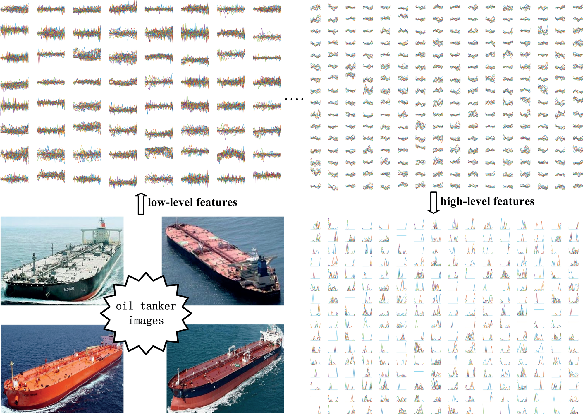
Figure 2. CNN-learned features at different levels for the ship type of oil tanker.
The ship features of convolution layer outputs can be classified as trivial and non-trivial features, which have different influences on the ship type recognition task. More specifically, the trivial features of the ships do not provide very useful information for identifying ship types, while training on these unimportant ship features results in significant increase of computation cost. To mitigate the disadvantage, the pooling layers are designed to help the CNN model concentrate on the non-trivial ship features. We employ the max-pooling method to pool the non-trivial ship features obtained from the convolutional layers. The pooled features are obtained with Equation (2) as follows:
 $$P_{u,v} =\max _{i\in \left[ {1,k} \right],j\in \left[ {1,k} \right]} S_{n\left\{ {i+\left( {u-1} \right)\times d,j+\left( {v-1} \right)\times d} \right\}s}^r$$
where k is the pooling kernel size, parameter d represents the stride step, and  $S_{n}^{r} $ is the nth ship feature map obtained from the previous convolution layer. The corresponding pooling feature map of
  $S_{n}^{r} $ is P u, v. Parameters u and v are the dimensions of P u, v.
The LRN layers are added into the CNN's hidden layers to help the DL model achieve satisfactory accuracy of ship recognition. More specifically, the LRN layers enable the CNN to obtain more generalised ship features based on the outputs from the previous layers. The response normalisation function for a fixed feature value  $\Gamma_{i}^{r}$ in the LRN layer is shown as Equation (3):
 $$\Phi _i^r = \displaystyle{{\Gamma _i^r } \over {(a + \eta \sum\nolimits_{j = {\rm max}(0,1-h/2)}^{{\rm min}(U-1,i + h/2)} {\Gamma _j^2 )^\varphi } }}$$
where  $\Phi_{i}^{r} $ is the response of the ith ship feature map at the rth LRN layer,
  $\Gamma_{i}^{r}$ represents a specified feature value of the ith ship feature map at the rth LRN layer, parameters a, η, φ and h are hyper-parameters in the CNN, and U is the number of ship types.
After implementing the feature learning process conducted by the above layers, the CNN can obtain generalised and distinctive feature maps for each ship type. The fully connected layers are then devised to assist the CNN model to understand the ships' features and patterns. Factually, the fully connected layers convert the extracted ship features into a long ship feature vector (i.e., one-dimension vector) (Hu et al., Reference Hu, Zhuo, Zhang and Li2017). We can obtain the output ship feature vector of the FC layer as Eq. (4).
 $$F_{{\rm out}} ={\Theta }\times F_{{\rm in}}$$
where F out is the output ship feature vector in the FC layer involving n 1 elements, and F in is the input ship feature vector with n 2 elements. Parameter Θ is a connecting matrix which concatenates F in and F out, with the dimension of n 1 × (n 2 + 1).
The final layer of the CNN model is the SoftMax layer, which is deployed after the FC layer. The role of the SoftMax layer is to determine the ship type of the initial input image according to the confidence values. More specifically, based on the ship features obtained from the previous FC layer, the SoftMax layer generates a probability vector for the input ship image. The CNN considers the ship type with the largest value in the probability vector as the predicted ship category. For an input ship image, the CNN classifies the ship as the ith category with the following probability distributions (see Eq. (5)).
 $$P_i =\frac{e^{( {v_i F_p } ) }}{\sum\nolimits_{j=1}^U {e^{( {v_j F_p } ) }} }$$
where F p is the ship feature vector obtained from the previous layer, and v j is the weight for the jth ship type, where parameter V is the weight set [v 1, v 2, …v U].
2.2. CFCCNN for ship type recognition
Note that the over-fitting phenomenon is a common shortcoming of conventional CNN models, which may degrade the performance of the CNN in the ship recognition task. For the purpose of mitigating the disadvantages of CNN methods, previous studies proposed regularisation-based methods (data augmentation, dropout and dropconnect, etc.) to extract more intrinsic features by generating more training samples, deactivating neurons etc. (Krishevsky et al., Reference Krishevsky, Sutskever and Hinton2012). The data augmentation mechanism increases the number of ship training samples by implementing operations of translation, rotation and scale transformation on the initial training images of ships (Guo and Gould, Reference Guo and Gould2015). Dropout and dropconnect are two newly developed regularisation approaches which have achieved satisfactory performance in addressing the CNN over-fitting challenge (Hinton et al., Reference Hinton, Srivastava, Krishevsky, Sutskever and Salakhutdinov2012; Wan et al., Reference Wan, Zeiler, Zhang, Le Cun and Fergus2013). Motivated by the success of the previous studies, we proposed the CFCCNN framework for fulfilling the ship type recognition task; it consists of three main steps: formatting the input training ship images and labels, implementing training procedure and recognising ship type based on the confidence level (i.e., the outputs of implementing the FC layer and SoftMax layer). The first step aims to provide trainable ship data for the CFCCNN model, which works in a similar way to the standard CNN model. The second step (i.e., training procedure) is to find distinct ship features with optimal parameter settings in CFCCNN (which is critical for the recognition performance). The third step works in a similar way to conventional CNN. Overall, we will concentrate on the CFCCNN training procedure due to this step being more crucial for the ship type recognition performance (while the first and the third steps are very similar to those of conventional CNN). The proposed framework overview is shown in Figure 3.

Figure 3. Framework of the proposed CFCCNN.
For each cascaded layer in the CFCCNN model, the coarse step and fine step are implemented in a nesting manner. More specifically, the coarse step of the CFCCNN is fed with training images of ships (and features) from all of the ship types (or the outputs from the previous cascaded layer), and is then trained to extract distinct ship features. The training process of the coarse step of the CFCCNN is similar to that of the standard CNN, and the fine step is implemented to improve the recognition performance of the ship type that had the lowest recognition accuracy in the coarse step. It is noted that the coarse step may fail to achieve satisfactory recognition accuracy due to lack of sufficiently diverse training samples of ships. The regularisation methods (i.e. data augmentation, dropconnect and dropout mechanism) are introduced in the fine step for mitigating such disadvantage.
Considering the Vth ship type obtaining the lowest recognition accuracy, the CFCCNN is being further fine-tuned in the fine step based on the training data (i.e., images and labels) of the Vth ship type. More specifically, we propose an RHS mechanism to select an appropriate regularisation method to generate significant additional training samples of ships and extractable ship features, and thus extract more intrinsic ship features. The RHS mechanism selects one of the three regularization methods based on probability (see Eq. (6)).
 $$\begin{aligned} & P_{is} =\mbox{Max} \lcub {\omega_{i1} \times \theta_{ir} +\omega_{i2} \times \theta_{ih} } \cub \\ & \mbox{s.t.} \begin{cases} {\sum\limits_{i=1}^3 {[\omega _{i1} \times \theta _{ir} +\omega _{i2} \times \theta _{ih} ]=1} } \\ {\omega _{i1} +\omega _{i2} =1 } \\ {\theta _{ih} =\dfrac{1}{N_i }\times P_{ia} } \\ {\omega _{i1} \le \omega _{i2} } \\ {\omega _{i1} \ge 0 } \\ {\omega _{i2} \ge 0 } \\ {i=1,2,3 } \end{cases} \end{aligned}$$
where P is is the probability of choosing the ith regularisation method. The sequences for the data augmentation, dropout and dropconnect methods are marked as 1, 2 and 3, respectively. Parameter θir is the random factor and θi is the heuristic factor, both of which are used for selecting the ith regularisation approach. Parameters ω i1 and ω i2 represent the weight factor for θ ir and θ i, respectively. N i is the training image number of the input ship type. For the ith ship type, P ia is the difference in recognition accuracy of implementing or not implementing the fine step in the CFCCNN model.
The probability of selecting a regularising model relies on the addition result of the random selection component ωi1 × θir and heuristic component ωi2 × θih. Initially, the RHS mechanism randomly selects a regularising approach due to no prior knowledge being available. The ω i2 value will then adaptively increase or decrease according to the variation of recognition accuracy P ia (as shown in Equations (7) and (8)). Specifically, the current heuristic ω i2 equals the sum of P ia and the previous heuristic counterpart. Thus, a positive value for P ia will lead to a higher probability of choosing the ith regularisation method, and vice versa. The CFCCNN will stop the fine step when one of the following criteria is met: (1) a higher recognition accuracy for the Vth ship type is obtained; (2) the three regularisation models are selected and implemented, and thus the operation in a cascaded layer is considered as finished.
Note that when the ship type with the worst recognition accuracy has been continuously selected several times (more than the threshold s m), the fine step of the CFCCNN will adaptively choose the ship type with the second-worst recognition accuracy for analysis. We set s m to 3 because the RHS mechanism in the CFCCNN fine step can only select the regularisation method from the models of data augmentation, dropout and dropconnect. The CFCCNN model will terminate when one of the following conditions is satisfied: (1) the number of CFCCNN cascaded layers N cl reaches the maximal threshold; (2) the difference between the recognition accuracy of the neighbouring CFCCNN coarse steps is smaller than a threshold θ c in consecutive N d times. The output of the training step in CFCCNN is a well-trained recognition model, which can be directly used to fulfil the ship recognition task.
3. EXPERIMENTS
3.1. Data and experimental setting
3.1.1. Data
Several image sets of merchant ships are available for the ship recognition task. For instance, the dataset of the IMAGENET Large Scale Visual Recognition Challenge 2012 (ILSVRC-2012) provides a bank of images of ships. However, only one type of merchant ship (i.e., container ship) is inclued in the ship images in the ILVSVRC-2012; the other ship images in ILVSVRC-2012 are of yachts, fireboats, drilling platforms etc. (Russakovsky et al., Reference Russakovsky, Deng, Su, Krause, Satheesh, Ma, Huang, Karpathy, Khosla, Bernstein, Berg and Fei-Fei2015). Recognising different categories of merchant ships is more important, however, as a large proportion of ships sailing in waterways are merchant ships. Hence, our team collected images of seven types of merchant ships. With the help of our group members (i.e., graduate students), we manually collected images of seven types of merchant ships from free online image-sharing websites, regardless of size and sailing direction of the ships. We modified the resolution of each image to 512*512, and each image was manually labelled and checked by an experienced ship's captain in our group. We did not collect ship data from maritime surveillance videos (such as VTS, CCTV) due to its sensitivity.
The first six types of merchant ships are: container ship, oil tanker, chemical carrier, LNG tanker, general cargo ship and bulk carrier. These six categories of ships are common merchant ship types in the maritime community. The seventh ship type is composed of a set of ship types that are less frequently encountered. The gathered images for the seventh ship type include: timber carrier, barge carrier, refrigerator ship etc. For clarity, the first six types of ships are labelled by the name of the ship category, and the seventh type is labelled ‘others’. In our image set, the number of images of the first six ship types are 2,720, 1,320, 1,600, 1,200, 2,850 and 2,070, respectively. We collected 1,560 images for the seventh ship type. For each ship type, we selected 80% of the images as the training set, and the remaining 20% were used as the testing set. Some samples of the collected ship images are shown in Figure 4.

Figure 4. Samples of images collected for each type of ship.
3.1.2. Platform and parameter settings
We applied the proposed deep CNN to recognise the above-mentioned ship types. The CFCCNN model was implemented on a system with Windows 10 OS, 16 GB of RAM and 3·4 GHz of CPU. We employed MATLAB (R2016 version) to perform the simulations. It is known that training a CNN is a time-consuming task due to a large number of parameters in the network. A common trick to reduce the training cost is to train a discriminative CNN based on some pre-trained CNNs (Long et al., Reference Long, Shelhamer and Darrell2015; Ma et al., Reference Ma, Dai, He, Ma, Wang and Wang2017). Many researchers have theoretically proven the reasonability of the CNN training logic (Razavian et al., Reference Razavian, Azispour, Sullivan and Carlsson2014; Yosinski et al., Reference Yosinski, Clune, Bengio and Lipson2014). Inspired by the performance of the Cafe model in object classification tasks, we trained our CFCCNN based on the pre-trained Cafe model (Jia et al., Reference Jia, Shelhamer, Donahue, Karayev, Long, Girshick, Guadarrama and Darrell2014). Some basic parameters of the CFCCNN are listed in Table 1.
Table 1. Initial parameter settings for the CFCCNN.

Note: aWhere N bz represents the number of batch size, N ep is the epoch number, σwd is the weight decay and σlr is the learning rate. f cl and f pl represent the filter size used in the convolution layers and pooling layers, respectively.
Previous studies show that setting appropriate values for hyper-parameters is critical for CNN based model performance (Donahue et al., Reference Donahue, Jia, Vinyals, Hoffman, Zhang, Tzeng and Darrell2014; Fang et al., Reference Fang, Zhou, Yu and Du2017; Ma et al., Reference Ma, Dai, He, Ma, Wang and Wang2017). A minor change in the CFCCNN's hyper-parameters, including batch size, weight decay, learning rate and epoch, would lead to noticeable variations in recognition accuracy. Thus we employed a trial-and-error mechanism to determine proper settings for the above four hyper-parameters in the CFCCNN (Bei et al., Reference Bei, Chen and Zhang2013). Two common indicators, 1-type error and 5-type error, were used to evaluate the recognition performance of the CFCCNN. The 1-type error is detailed as follows. Given a test image of a ship from the image set, the CFCCNN recognition output is a confidence level map. Specifically, each type was assigned a recognition probability for the input ship image. To assess the 1-type error, the CFCCNN labels the to-be-recognised ship as the type with the highest probability. The 1-type error is calculated by Equation (7):
 $$e_{1t} =\frac{N_{er} }{N_s }$$
where N s is the number of ship images and N er represents the number of ship images with erroneous recognition results. In addition, the CFCCNN considered the labels with the top five recognition probabilities as the recognised ship types for evaluating the 5-type error. The 5-type error can be obtained in a similar way to the 1-type error.
Figure 5 demonstrates the error distributions of the CFCCNN recognition results with different hyper-parameter settings. We can observe that inappropriate settings for the four parameters significantly degraded the recognition performance of the CFCCNN. Subplot (a) in Figure 5 shows that the optimal setting for the batch size is 15. More specifically, the recognition error, in terms of the 1-type error, experienced a decreasing trend when the batch size increased from 5 to 15, however, the recognition error climbed sharply when the batch size increased from 15 to 50. Moreover, the 1-type error reached almost 40% when the batch size was 50. The 5-type error showed an error variation tendency similar to that of the variation of 1-type error. Therefore, we set 15 as the default value for the batch size in the CFCCNN model. The variation of the weight decay, demonstrated in the subplot (b) in Figure 5, showed that the minimal recognition error was obtained when the weight decay equalled 5 × 10⁻⁴. In particular, the 1-type error declined to 10% when the weight decay was set to 5 × 10⁻⁴. From the perspective of the 5-type error, the recognition accuracy of the CFCCNN did not fluctuate significantly under variations of weight decay. Thus, the default weight decay is 5 × 10⁻⁴ in our research.

Figure 5. Recognition performance of CFCCNN under different parameter settings: (a) distributions of recognition error at different settings of batch size; (b) distributions of recognition error at different settings of weight decay; (c) distributions of recognition error at different settings of learning rate; (d) distributions of recognition error at different settings of epoch.
The value of the learning rate decreased from 2 × 10⁻¹ to 2 × 10⁻⁷, and the stride step is 1 × 10⁻¹. Subplot (c) in Figure 5 illustrates that the 5-type error did not vary significantly with different settings of learning rate. However, the 1-type error shrank from 22% to approximately 15% when the learning rate decreased from 2 × 10⁻¹ to 2 × 10⁻³. The 1-type error then showed a minor variation when the learning rate changed from 2 × 10⁻³ to 2 × 10⁻⁷, however, the convergent time of the CFCCNN was much longer when the learning rate was smaller than 2 × 10⁻³. Thus, the optimal value of the learning rate in the CFCCNN is 2 × 10⁻³. Compared with the above three parameters, the variation in the epoch did not have considerable influence on the recognition performance of the CFCCNN. Subplot (d) in Figure 5 shows that the CFCCNN reached a stable recognition performance when the number of epoch was not less than 200. Hence, the default epoch number in our research is set to 200 without further specifications.
3.2. Analysis of CFCCNN performance on recognition of ship types
Container ships, general cargo ships and oil tankers are the most commonly encountered ship types in coastal waterways, and Figure 6 shows the CFCCNN recognition results for the three typical ship categories. Subplot (a) of Figure 6 shows a typical image of a container ship and the corresponding CFCCNN recognition results. As shown in the right subplot of Figure 6(a), the corresponding confidence level for the container ship is 97·8%, and the counterpart for the general cargo ship is 2·2%. Additionally, the confidence levels for the other four ship types are 0·0%. Thus, the CFCCNN can easily determine that the input ship image belongs to the type of container ship. In addition, the above confidence level distribution also suggested that the CFCCNN has gained the most significant features from the training images of container ships.

Figure 6. Recognition results of CFCCNN for typical ship types: (a) Typical image of a container ship and its recognition result; (b) Typical image of a general cargo ship and its recognition result; (c) Typical image of an oil tanker and its recognition result.
The second subplot of Figure 6 reveals a test image of a general cargo ship and the corresponding CFCCNN recognition results. It is evident that there is a crane mounted on the ship. Usually, both general cargo ships and small-size bulk carriers are equipped with cranes. However, hatches are essential components in bulk carriers, whereas general cargo ships are not equipped with such facilities. The features of cranes and hatches help the CFCCNN to distinguish general cargo ships from bulk carriers and other ship types easily. The confidence level distributions for the test image of a general cargo ship confirmed the above analysis. From subplot (b) in Figure 6, the confidence level for the type of general cargo ship is 99·6% and 0·4% for that of bulk carrier. Thus, we can conclude that the CFCCNN has successfully extracted and learned in-depth features of the ship type of general cargo ships.
The last sub-figure in Figure 6 shows the CFCCNN recognition results for an oil tanker. It is common sense that the appearance of an oil tanker and that of a chemical carrier are similar. From the perspective of a ship's crew, the pipelines above the deck of a chemical carrier are more complicated than those of an oil tanker. It is challenging, however, to describe quantitatively the difference between chemical carriers' pipelines and those of oil tankers. In this case, the robust generalisation capability enables the CFCCNN to extract and learn such complex differences between the two types of ships. As shown in subplot (c) of Figure 6, the confidence level for the type of oil tanker equalled 96·4%, and the counterpart for the type of chemical carrier ship was just 3·6%. The confidence level distributions have confirmed our above analysis.
We have also presented the overall recognition results for different ship types, as listed in Figure 7. We employed Equation (8) to calculate the accuracy of recognition of single ship type, and Equation (8) to obtain the average recognition accuracy of all the ship types. Figure 7 shows that the seventh ship type obtained the highest recognition accuracy, which was 93·3%. This is because ships of the seventh ship type possess more distinctive features. For instance, roll on/roll off (R/R) ships, belonging to the seventh type, usually load smaller-sized vehicles. Hence, the textures and contours of R/R ships are different from other types of ships. The CFCCNN can easily catch such distinctive R/R ship features. Thus, it is reasonable that the seventh ship type obtained a higher accuracy compared with the other six ship types.

Figure 7. Recognition accuracy of CFCCNN for different ship types.
 $$A_a =\frac{\sum_{i=1}^7 {A_i \ast N_i }}{\sum_{i=1}^7 {N_i } }$$
where A i is the recognition accuracy for the ith ship type, N i is the number of images for the ith ship type, and A a represents the average recognition accuracy considering all the seven ship types.
In addition, we observed that recognition accuracies for the three most important merchant ship types (general cargo ships, container ships and oil tankers) were greater than 80%. More specifically, the recognition accuracy for the container ships was 90·7% and 86% for the general cargo ships. The reason for the high accuracy of recognition of these two ship types is that the container ships and general cargo ships have more obvious visible features than other ship types. For instance, the majority of pixels in container ship images are containers which have distinctive extractable contours (i.e., rectangles), and thus can be easily learned and recognised by the CFCCNN model. Table 2 also shows that the recognition accuracies for chemical tankers and LNG tankers are much lower than those of the other types (which are 65·6% and 66·7%, respectively). It is noticed that the visible difference in appearance between oil tankers and chemical tankers is not so significant compared with other ship types, and CFCCNN may obtain incorrect recognition results by falsely recognising a chemical tanker as an oil tanker. The reason for the lower recognition accuracy for LNG ships is that the CFCCNN identified some LNG ships as the seventh ship category. Though the recognition accuracy for chemical ships and LNG tankers is not high, the CFCCNN model achieved an average accuracy at 81·4%, which is considered satisfactory.
Table 2. Recognition performance achieved by CFCCNN and other algorithms.

To further verify our model's performance, we implemented other popular models on the task of recognising ship types. For the purpose of model comparison, the parameter settings of the CFCCNN model are provided as follows: the weight factor ω i1 and ωi1 (i = 1, 2, 3) are both set as 0·5, and the initial heuristic factor θih (i = 1, 2, 3) is set to 0. The parameter settings of batch size, weight decay, learning rate and epoch are set to optimal values, which are 15, 5 × 10⁻⁴, 2 × 10⁻³ and 200. For more detailed parameter settings, refer to the platform and parameter settings section. Table 2 shows the accuracy of ship recognition by: k-nearest neighbour (KNN) (Jiang et al., Reference Jiang, Pang, Wu and Kuang2003), artificial neural network (ANN) (Reda and Aoued, Reference Reda and Aoued2014), random forest (RF) (Wang et al., Reference Wang, Wang and Zhao2010) and standard CNN (Krishevsky et al., Reference Krishevsky, Sutskever and Hinton2012). Note that we followed the parameter setting rule for each model in the previous studies. It is noticed that our proposed ship type recognition framework outperforms the non-CNN models, and the reasons are provided as follows: (1) the uneven training sample size for each ship type leads KNN to set biased weights in the feature learning procedure, which results in learning biased features for each ship type. The training procedure of the proposed CFCCNN is not affected by the training sample size, and the features of each ship type are independently learned with equal weights. The ANN method is easily trapped by the local optimal solution, and thus the learned ship features may vary at different iterations. Our model is trained to explore the global distinctive features of each ship type, with the input training data being learned by cascaded layers in ANN. The RF model is an ensemble classifier involving several weak classifiers, and the model will be interfered with when the visible appearances of different ship types are very similar (i.e., the extracted features are very similar). The CFCCNN model is not easily interfered with by similar features of different ship types, as the RHS mechanism generates more distinctive training data samples with the three regularisation methods.
Table 2 also shows that our proposed ship recognition model outperforms the standard CNN method. From the perspective of the three typical ship types, the average recognition accuracy of the CFCCNN was approximately 5·0% higher than the counterpart of the standard CNN. Specifically, the recognition accuracy of CNN for the type of general cargo ships was 80·0%, which was 6·0% lower than that of the CFCCNN. The recognition accuracy of CFCCNN and the CNN for oil tankers showed a gap similar to their recognition accuracy of general cargo ships. The recognition accuracy of the container ships by CFCCNN was better than the CNN counterpart by 5·5%. It can be inferred that the over-fitting phenomenon often happens in the traditional CNN, which means the input ship data (images, labels, etc.) are over-trained, and thus the noises in the input data are also learned as distinctive ship features. The proposed CFCCNN model mitigates the disadvantage of traditional CNN by implementing the three regularisation models. By carefully checking the CFCCNN recognition results, we found 43% of ship images were recognised by data augmentation regularisation, and 29% and 28% of ship images were recognised by the dropout and dropconnect mechanisms, respectively. The main reason for the selection of data augmentation as regularisation mechanism (by the CFCCNN model) with higher probability is that the data augmentation mechanism can provide more intrinsic ship features (by generating additional training ship images) against the geometric and photometric distortions and shifting interferences. In contrast, the dropout and dropconnect mechanisms tried to enhance the model recognition performance by deactivating the neuron, which did not actually introduce new learnable ship features, and thus may fail to obtain better performance than that of the data augmentation model (i.e., with lower probability being selected as the regularisation method by the CFCCNN model). Figure 8 displays a comparison of model performance between the CFCCNN and its counterparts in a clearer manner, and also presents the average recognition results for each model.

Figure 8. Recognition results achieved by different models on different ship types.
4. CONCLUSION
We proposed a CFCCNN for the task of ship type recognition, which involves two steps. The first step of the proposed deep network follows training logic similar to a traditional CNN. More specifically, we obtained the recognition performance for all ship types in this step. We called the first step the coarse step. The second step of the proposed deep network then identified the ship type with the lowest recognition accuracy, and the network was re-trained and fine-tuned. The second step was named the fine step. The fine step attempted to search for and extract more intrinsic features for the ship type with the worst recognition performance in the previous step. We integrated three efficient normalisation techniques into the fine step to obtain higher recognition accuracy. An RHS mechanism was developed to help the proposed CNN select a proper regularisation technique. The system completed a cascaded procedure after the proposed CNN finished the training process of the fine step. Another round of cascaded processes was performed in the proposed deep network until the stop criterion was met.
The recognition performance for the ship images indicated a satisfactory accuracy. In particular, our developed deep framework can recognise general cargo ships, oil tankers and container ships, which are the three most important types of merchant ships, at accuracies of 86·0%, 84·6% and 90·7%, respectively. Additionally, the average recognition accuracy of our proposed CNN was 81·4%. We also implemented three popular non-CNN structure models and a conventional CNN method in the ship type recognition task. The recognition results showed that the non-CNN methods fell behind the CNN models. Additionally, the conventional CNN model achieved lower ship recognition accuracy than our model. Specifically, the average recognition accuracy of the traditional CNN was 5% lower than that of our proposed CNN.
In the future, we will expand our study in the following directions. First, our model works well for recognising oil tankers, however, its performance at recognising chemical carriers is not as good as for oil tankers. Hence, we will investigate ways of revising our model to explore more distinguishable features for chemical carriers. Second, we may split the ship types into more refined levels to obtain higher recognition performances. Third, the proposed framework enhances the performance of traditional CNN by adding more positive samples with the RHS mechanism. In future, it would be interesting to enhance the model's performance by training the model with adversarial ship samples. Fourth, we have compared our model with other typical ship type recognition methods (KNN, ANN, RF, CNN) for the purpose of performance tests. It would be interesting to evaluate model performance against the other regularisation-improved (such as data augmentation, dropout, dropconnect) DL methods in our future study. Last but not least, we will seek to cooperate with maritime administration departments to collect videos of ships, and thus further verify the performance of our model in real applications.
ACKNOWLEDGEMENTS
This work was jointly supported by the National Natural Science Foundation of China (51709167, 41505001, 51579143) and the Shanghai Committee of Science and Technology, China (18040501700, 18295801100, 17595810300).


