


1. Introduction
The inertial navigation system (INS) is an independent system which performs navigation tasks with high reliability. Such a system utilises specific forces (accelerometer output) and angular rates (gyro output) in three dimensions. Nonetheless, considering the intrinsic bias errors of gyros and accelerometers, INS is usually unable to perform navigation tasks independently in the presence of such gradually increasing errors (Wu and Wang, Reference Whitcomb, Yoerger and Singh2013; Ning et al., Reference Mirabadi, Schmid and Mort2015; Shabani and Gholami, Reference Semeniuk and Noureldin2016). Hence, INS should adopt auxiliary sensors in order to provide the required measurements for improving navigation performance.
Integrated navigation systems are extensively utilised to overcome the mentioned drawback of INS. The integrated system depends on several auxiliary sensors which directly affect the accuracy of navigation (Niu et al., Reference Ning2007; Davari and Gholami, Reference Davari and Gholami2017). Once the sensors fail or are corrupted by fault, the navigation system tends to be unstable. In recent years, to cope with auxiliary sensor malfunctions, fault-tolerant schemes (FTS) have been developed, offering two groups of solutions. In the first, the faulty sensor is masked and replaced with redundant hardware, which leads to tremendous hardware cost (Brumback and Srinath, Reference Brumback and Srinath1987a; Mirabadi et al., Reference Lin1998; Li and Zhang, Reference Li2010; Ushaq and Cheng, Reference Shabani and Gholami2014). The other uses analytical redundancy to achieve reasonably cost-effective solutions (Semeniuk and Noureldin, Reference Pham and Yang2006; Li and Zhang, Reference Li2010; Hasan et al., Reference Hasan2011). Both of these methods require knowledge of the characteristics of faults in signals, which are usually determined by fault detection systems. The existing fault detection methods can be broadly classified into: analytical model-based, data-driven and knowledge-based methods. The analytical model-based approaches (Lin et al., Reference Li and Zhang2018) process the information by having the known mathematic model of a system and extracting the fault characteristic. Kalman filtering (Ansari-Rad et al., Reference Ansari-Rad, Kalhor and Araabi2019b), strong tracking filtering (Ansari-Rad et al., Reference Ansari-Rad, Kalhor and Araabi2019b) and chi-squared test statistics (Brumback and Srinath, Reference Brumback and Srinath1987b; Joerger and Pervan, Reference Joerger and Pervan2013) are the methods one can mention in this category. Employing these model-based approaches for constructing a practical fault detection method is difficult for complex vehicles because of complex dynamics and numerous sensors required for identification. On the other hand, the data-driven methods (Zabihi-Hesari et al., Reference Youssef2019) detect the fault by extracting variance, amplitude and frequency from the auxiliary sensors, based on signal processing methods such as wavelet transformation (Youssef, Reference Yao2002; Yan et al. Reference Xu, Li and Liu2014) and auto-regressive moving average (Pham and Yang, Reference Oh2010). Hence, reliable feature sets, decision criteria and large amounts of data are required to demonstrate objective outcome. In contrast to the mentioned methods (model-based and data-driven), knowledge-based approaches (Pham and Yang, Reference Oh2010) are drawing increasing attention from researchers due to their high intelligence and adaptable structures, which make them suitable candidates for application to navigation systems. Therefore, intelligent knowledge-based modules have been considered by some researchers (e.g., Xu et al., Reference Wu2015; Li et al., Reference Li and Zhang2017; Yao et al., Reference Yan, Gao and Chen2017) recently for constructing fault detection systems.
In order to increase the reliability of integrated navigation systems, both fault detection and FTS are required. However, few studies deal with fault detection and FTS design in integrated navigation systems. For fault detection in a GPS/INS integrated system, the residual signal is generated and statistical analysis reveals the fault characteristic (Oh et al., Reference Niu, Nassar and El-Sheimy2005). The fault detection scheme has been applied to a GPS/INS/magnetic compass integration system with statistical test related to azimuth error output (Oh et al., Reference Niu, Nassar and El-Sheimy2005). The fault detection scheme is achieved by training a Gaussian process regression (GPR) model to predict the innovation of a Kalman filter (Zhu et al., Reference Zabihi-Hesari2016). The fault can be detected by change in the mean value of innovation and the predicted innovation difference. In all mentioned references, the faulty sensor is masked to cope with sensor malfunctions. There must be an additional auxiliary sensor in addition to the faulty sensor to prevent system divergence in the mentioned strategy. Therefore, the mentioned references fall into the hardware redundancy strategy for FTS systems.
This paper investigates fault detection and FTS design in an INS/DVL integrated navigation system. In ocean navigation, since satellite signals are repeatedly attenuated, and GPS signals are unavailable, it is necessary to adopt other auxiliary sensors. For underwater navigation, Doppler velocity log (DVL) measures velocity with respect to the seafloor based on the Doppler effect, with high precision (Wu et al., Reference Wu and Wang2019). The emission of acoustic waves by wave-absorbing materials, or large roll and pitch caused by angular manoeuvres, are causes of malfunction of this sensor. Therefore, underwater vehicles may encounter gradual or sudden faults in DVL signals, contamination of the integrated and feedback data, INS error accumulation, and eventually inaccuracy in the integrated navigating system. Another aspect is that there is no other auxiliary sensor to prevent system divergence in underwater navigation. Seemingly, fault detection and FTS are indispensable to promote the reliability and safety of this navigation system. In Whitcomb et al. (Reference Ushaq and Cheng1999) a hybrid Least squares regression (LSR)-support vector regression (SVR) predictor was employed to handle short-term DVL outage. However, long-term malfunctions cause significant drop of the predictor performance. To avoid this drawback, evolutionary knowledge-based methods should be adopted in building the pseudo DVL structure. In Whitcomb et al. (Reference Ushaq and Cheng1999) a FTS for integrated navigation systems based on evolutionary artificial neural networks was considered to avoid short-term DVL malfunction drawback. The aforementioned evolutionary approach is only designed to be applied in cases where, during DVL malfunctions, magnetic compass data are available. In the mentioned references, analytical redundancy is used for FTS without considering fault detection procedure.
Despite the mentioned references, in this paper the FTS method is performed by replacing the faulty sensor with an analytical sensor (pseudo sensor) after the fault detection system finds the fault occurrence. Recently we designed an improved evolutionary TS-fuzzy (I-eTS) algorithm, with self-adaptation and online process of the system structure, to be used for reconstruction of DVL signals at moments when faults occur (Ansari-Rad et al., Reference Ansari-Rad, Hashemi and Salarieh2019a). This paper adopts an algorithm to reconstruct DVL signals by evolutionary TS-fuzzy (I-eTS) to improve fault tolerance for INS/DVL. It was shown that the I-eTS has superiority in long-term DVL malfunction with respect to existing methods. To check the advantages and probable disadvantages of I-eTS in the practical navigation system, the fault detection scheme is invoked by adopting the GPR model in this paper. The GPR model requires a training phase to find the GPR hyper-parameters, which is done by particle swarm optimisation (PSO) in this paper. Moreover, implementing this, a novel fault-detection-based FTS for INS/DVL is obtained in such a way that by detection of a fault in DVL signals with GPR models, a pseudo DVL sensor, trained by I-eTS, is substituted for the faulty DVL sensor in long-term DVL malfunctions. Consequently, the drawbacks of the mentioned ocean navigation system will be solved in the faulty condition.
The interaction between fault detection and FTS in the integrated navigation system is studied in this paper for the first time. Among other factors, the delay between the occurrence and detection of a fault, which is very important since it can lead to instability of the FTS, has not yet been studied in navigation systems.
The remainder of paper is organised as follows. Section 2 shows the structure of the INS error dynamics and integration system by extended Kalman filter. In Section 3, the fault detection methodology is comprehensively introduced. Subsequently, the I-eTS algorithm and the PSO are described as the evolutionary prior-knowledge learning methods in Section 4. The structure of the fusion FTS is presented in Section 5. Finally, Section 6 presents the simulation and field test results.
2. INS/DVL integrated navigation system
In this paper, extended Kalman filter (EKF) is used as the integration filter, but other types of KF, like UKF, could be used for this purpose without losing any generality. Figure 1 shows the block diagram of the INS/DVL navigation system in the loss of GPS signals and any fault detection mechanism.

Figure 1. Block diagram of the integrated navigation system with loss of fault detection and fault-tolerant mechanisms (Ansari-Rad et al., Reference Ansari-Rad, Hashemi and Salarieh2019a)
Intended to fuse navigation data, the 15-state space EKF is implemented, which contains the following elements:
 \begin{equation}x = {[{\delta L\;\; \delta l\; \;\delta h\; \;\delta V_{\textrm{NED}}^{T\; }\; \;{{\tilde{\varepsilon }}^T}\; \;b_a^T\; \;b_g^T} ]^T}\; \end{equation}
where the  $\delta $ denotes the variation operator and
  $h,l,\; L$ are the height, longitude and latitude, respectively. The vehicle is expressed by
  ${V_{\textrm{NED}}} = {[{{V_N}\; {V_E}\; {V_D}} ]^T} \in {{{\mathbb R}}^{3 \times 1}}$ in north, east and down directions in the known North-East-Down (NED) frame. Moreover,
  ${\tilde{\varepsilon } } \in {{{\mathbb R}}^{3 \times 1}}$ is the vector of the perturbed quaternion;
  $b_a \in {{{\mathbb R}}^{3 \times 1}}$ and
  $b_g \in {{{\mathbb R}}^{3 \times 1}}$ represent the three-dimensional accelerometer and gyro biases in the body frame, respectively. For the definition of frames, refer to Karmozdi et al. (Reference Karmozdi, Hashemi and Salarieh2018).
The state space nonlinear model based on the perturbed INS mechanism is formulated as follows (Karmozdi et al., Reference Karmozdi, Hashemi and Salarieh2018):
 \begin{equation}\begin{aligned} \dot{x} & =f({x,u} )+ \xi (t ),\quad \xi = \textrm{N}({0,\textrm{{\cal Q}}} )\\ z & =h(x )+ \kappa (t ),\quad \kappa = \textrm{N}({0,R} )\end{aligned}\end{equation}
where  $f({x,u} )\in {{{\mathbb R}}^{15 \times 1}}$ is the system vector and
  $h(x )\in {{{\mathbb R}}^{3 \times 1}}$ is the observation vector. Furthermore, u indicates the input vector and
  $z \in {{{\mathbb R}}^{3 \times 1}}$ is the measurement vector;
  $\xi \in {{{\mathbb R}}^{15 \times 1}}$ and
 $\; \kappa \in {{{\mathbb R}}^{3 \times 1}}$ are white process and measurement noise with covariance matrices
  $\textrm{{\cal Q}}$ and R, respectively. Bias instability in inertial sensors can also be modelled by a first-order Markov process. The discrete-time formulation of the system, described in Equation (2), is acquired by employing the forward Euler method. The state transition matrix is approximated at time step k, based on the following equation:
 \begin{equation}{{\Phi }_k} = {\textrm{I}_{k \times k}} + \frac{{\delta {f_k}}}{{\delta x_k^T}}({{x_k},{u_k}} ){\Delta }t\end{equation}
where  ${x_k},{u_k}$ are the system states, the system input vectors at stage k,
  ${\textrm{I}_{k \times k}}$ is the identity matrix with
  $k \times k$ dimension and
  ${\Delta }t$ is the discretisation time step. The measurement matrix is obtained as follows:
 \begin{equation}\theta _k^T = \frac{{\delta {z_k}}}{{\delta x_k^T}}({{x_k}} )\end{equation}
where the measurement vector at step k is represented by  ${z_k} \in {{{\mathbb R}}^{3 \times 1}}$. The EKF procedure has two separate parts: update and prediction. The Kalman gain
  ${K_k} \in {{{\mathbb R}}^{15 \times 3}}$ is computed at the first part. By using the prior estimate,
  $\hat{x}_k^ - $, and its error covariance,
  $P_k^ - $, the estimated state vector,
  $\hat{x}_k^ + $, and the error covariance matrix,
  $P_k^ + $, are updated, as seen in Equation (5). Moreover,
  ${\textrm{{\cal Q}}_k}$ and
  ${R_k}$ represent white noise covariance matrices for process and measurement (Chiang et al., Reference Chiang, Duong, Liao, Lai, Chang, Cai and Huang2012)
 \begin{equation}\begin{aligned} {K_k} & =P_k^ - \theta _k^T{({{\theta_k}P_k^ - \theta_k^T + {R_k}} )^{ - 1}}\\ \hat{x}_k^ + & =\hat{x}_k^ - + {K_k}{r_k}\\ P_k^ + & =({I - {K_k}{\theta_k}} )P_k^ - {({I - {K_k}{\theta_k}} )^T} + {K_k}{R_k}K_k^T. \end{aligned}\end{equation}
 In this regard,  ${r_k} \in {{{\mathbb R}}^{3 \times 1}}$, so-called Kalman innovation, in the update stage of step k can be calculated as seen in Equation (6). Moreover, the covariance matrix of Kalman innovation, denoted by
  ${{\Theta }_k} \in {{{\mathbb R}}^{3 \times 3}}$, is calculated, which is employed for the fault detection algorithm at Section 3 as follows
 \begin{equation}\begin{aligned} {r_k} & ={z_k} - {h_k}({\hat{x}_k^ - } )\\ {{\Theta }_\textrm{k}} & ={\theta _k}P_k^ + \theta _k^T + {R_k} \end{aligned}\end{equation}
At the second part, the prediction step is formulated as follows:
 \begin{equation}\begin{aligned} \hat{x}_{k + 1}^ - & ={f_k}({\hat{x}_k^ + ,{u_k}} )\\ P_{k + 1}^ - & ={{\Phi }_k}P_k^ + {\Phi }_k^T + {{\Omega }_k}{\textrm{{\cal Q}}_k}{\Omega }_k^T. \end{aligned}\end{equation}
3. DVL fault detection with GPR
In Section 2, the INS/DVL integrated system is introduced, where no fault or any interruption occurs during the updating and prediction stages. In this section, the detail of a fault detection mechanism is reviewed, intended to predict the Kalman innovation with a GPR model and to compare with information acquired from EKF.
The Kalman innovation vector,  ${r_k} \in {{{\mathbb R}}^{3 \times 1}}$, is also acquired from the EKF update stage from Equation (6). Nonetheless, each predicted value of Kalman innovation,
  ${r^\ast }$, which is the output of the GPR model is calculated as a scalar, trying to avoid the computational complexities that often occur in a multi-output GPR model. Details of how to calculate the
  ${r^\ast }$ from the GPR model and how to train the model by PSO can be found in Zhu et al. (Reference Zabihi-Hesari2016). Thus, one can write
  $r_k^\ast = {[{r_k^{\ast 1},r_k^{\ast 2},r_k^{\ast 3}} ]^T}$ and
  ${\Theta }_k^\ast = \textrm{diag}({{\Theta }_k^{\ast 1},{\Theta }_k^{\ast 2},{\Theta }_k^{\ast 3}} )$, where
  $r_k^{\ast i},i = 1,2,3$ and
  ${\Theta }_k^{\ast i},,i = 1,2,3$ are the predicted values of Kalman innovation and the corresponding covariance matrix. The independency of
  ${r_k}$ and
  $r_k^\ast \; $ is another important point to note, which by consideration of different sources of signals, is an acceptable assumption. Consequently, the prediction error of Kalman innovation,
  ${\sigma _k} \in {{{\mathbb R}}^{3 \times 1}}$, and the corresponding covariance,
  ${{\Sigma }_k} \in {{{\mathbb R}}^{3 \times 3}},$ is calculated at the
  ${k^{\textrm{th}}}$ step as follows:
 \begin{equation}\begin{aligned} {\sigma _k} & ={r_k} - r_k^\ast \\ {{\Sigma }_k} & ={{\Theta }_\textrm{k}} + {\Theta }_\textrm{k}^{\ast } \end{aligned}\end{equation}
 In this regard, in case of fault-free navigation,  ${F_0},$ the prediction error is a Gaussian white noise, with the following probability density function:
 \begin{equation}{P_r}({\eta |{F_0}} )= (1/\sqrt {2\pi } {\left|{\sum\limits_k {} } \right|^{1/2}}^{}exp \left( { - \frac{1}{2}\sigma_k^T\sum\limits_k^{ - 1} {{\sigma_k}} } \right),\; E\{{{\sigma_k}} \}= 0,\; E\{{{\sigma_k}\sigma_k^T} \}= {{\Sigma }_k}.\end{equation}
 However, if any type of fault occurs, whether abrupt or gradual, $\; {\textrm{F}_1}$, the mean value of the prediction error, deviates from zero, leading to the following probability density function:
 \begin{align}&P_{r}({\eta |{F_1}} )= \left(1/\sqrt {2\pi } {\left|{\sum\limits_k {} } \right|^{1/2}}\right)exp \left[ { - \frac{1}{2}{{({{\sigma_k} - \upsilon } )}^T}\sum\limits_k^{ - 1} {({{\sigma_k} - \upsilon } )} } \right],\notag\\ &E\{{{\sigma_k}} \}= \upsilon ,\; E\{{({{\sigma_k} - \upsilon } ){{({{\sigma_k} - \upsilon } )}^T}} \}= {{\Sigma }_k}\end{align}
where  $|{{{\Sigma }_k}} |$ indicates the determinant of prediction error covariance. The likelihood ratio of the fault, based on Neyman-Pearson lemma, is formulated as follows:
 \begin{equation}\ln {P_r}({{\sigma_k}|{F_1}} )/{P_r}({{\sigma_k}|{F_0}} )= 1/2\left[ {\sigma_k^T\sum\limits_k^{ - 1} {{\sigma_k} - {{({{\sigma_k} - \upsilon } )}^T}} \sum\limits_k^{ - 1} {({{\sigma_k} - \upsilon } )} } \right]\; \end{equation}
 If  $\upsilon = {\sigma _k}$, the above equation reaches its maximum value, leading to the following fault detection function
  $\textrm{(}{F_k})$:
 \begin{equation}{F_k} = \sigma _k^\textrm{T}\sum\limits_k^{ - 1} {{\sigma _k} = {{({{r_k} - r_k^\ast } )}^\textrm{T}}{{({{{\Theta }_\textrm{k}} + {\Theta }_\textrm{k}^{\ast }} )}^{ - 1}}({{r_k} - r_k^\ast } )} \end{equation}
 In the case of fault-free navigation,  ${\sigma _k}$ as the prediction error of the
  ${k^{\textrm{th}}}$ step keeps the fault detection function bounded within a specific range,
  ${F_k} \le {T_{rsh}}$, where
  ${T_{\textrm{rsh}}}$ should be defined by the user. Accordingly, by selecting a large threshold, the chance of missing a fault also increases. Conversely, a small assigned value may cause false alarms during fault detection procedure, demanding an optimal value for the threshold to be found to minimise the possibility of false alarm or missing the fault, consequently.
4. FTS based on fault detection
In this section, the structure of fault tolerance for INS/DVL is introduced. First, given the I-eTS algorithm introduced in Ansari-Rad et al. (Reference Ansari-Rad, Hashemi and Salarieh2019a), the AI-aided navigation system is developed. According to Figure 2(a), in the learning stage, required online information, including IMU, INS and  ${\Delta }{V_{\textrm{DVL}}}$, is employed in order to train the I-eTS network structure. While the I-eTS network undergoes the learning stage, EKF corrects the corresponding outputs and integrates the INS and DVL information. Moreover, in Figure 2,
  ${P_{\textrm{INS}}}$,
  ${V_{\textrm{INS}}}$ and
  ${q_{\textrm{INS}}}$ are the position, velocity and quaternions of INS sensor;
  $\delta P$,
  $\delta V$ and
  $\delta q$ denote the estimated variation of the parameters, obtained by EKF; and
  ${f_b}$ is the accelerometer outputs. In Figure 2(b), the case of an ideal FTS is demonstrated, where without any fault detection, the occurrence of any malfunctions in DVL signals is detected and the learning procedure of I-eTS is stopped. Afterwards, the well-trained network predicts the difference between DVL and INS velocity signals, constructing the so-called pseudo DVL signals
  ${\Delta }{V_{\textrm{pseudo} - \textrm{DVL}}}$. As a result, EKF exploits the predicted signals instead of the original damaged DVL signals to update INS outputs.

Figure 2. Ideal fault tolerance for INS/DVL integrated system. (a) Training phase of I-eTS in absence of fault detection procedure. (b) Ideal fault detection: employing pseudo DVL for INS/DVL integrated navigation
On the contrary to Figure 2, in the implementation stage, fault detection demands a high-precision mechanism to correctly identify the moments of malfunctions occurring. Without such a mechanism, any abrupt or gradual fault in DVL signals that passes through the I-eTS learning stage leads to the probable instability in navigation. Similarly, any delay in detecting such crucial moments leads to an impaired pseudo DVL estimator, which reduces the performance of the navigation system. Consequently, as employing an agile and high-performance fault detector seems necessary, such a mechanism should be in absolute cooperation with the I-eTS network in order simultaneously to detect the fault and switch from faulty DVL signals to the pseudo DVL signals. Therefore, the fault detection mechanism, introduced in Section 3, is utilised, converting the FTS for integrated navigation system into the one demonstrated in Figure 3, where the dashed lines indicate the information required for training procedures in both networks.

Figure 3. Fault detection in cooperation with the I-eTS network. (a) GPR training phase. (b) Fault detection structure: employing GPR prediction signals
In Figure 3(a), the training phase scheme of GPR models is shown in which  ${P_{\textrm{INS}}}$,
  ${V_{\textrm{INS}}}$,
  ${q_{\textrm{INS}}}$, as INS sensor information, and
  ${f_b}$, as the IMU data, construct the input data sets of GPR models, utilising the Kalman innovation vector, r, and undergo the PSO procedure in order to train precise models. Thereafter, in the GPR prediction stage, the predicted Kalman innovation vector and the corresponding covariance matrix are employed by the fault detection function (12), intended to compare with the threshold value. In the case of detecting any malfunction, the algorithm substitutes
  ${\Delta }{V_{\textrm{DVL}}}$ with
  ${\Delta }{V_{\textrm{pseudo} - \textrm{DVL}}}$, which constructs a novel FTS for the INS/DVL system. Such a system not only detects any malfunction from an auxiliary sensor, but also switches to reliable pseudo DVL signals, providing a similar performance to the fault-free conditions, which makes it an appropriate option for ocean navigation systems.
5. Results of field tests
To evaluate the performance of the introduced method, an instrumented vessel was equipped for the experiment, which is shown in Figure 4. The instruments include a MEMS IMU, DVLs and a GPS receiver, as shown in Figure 4. GPS measurements were used for the navigation initialisation process and as a reference for comparison of navigation results. The specifications of the sensors can be found in Table 1.

Figure 4. Instrumented vessel for field test (left) and instruments mounted on the vessel (right) (Ansari-Rad et al., Reference Ansari-Rad, Hashemi and Salarieh2019a)
Table 1. Instrument specifications

In the following, three different parts are devoted to the scenarios of experimental tests. First, considering the approach introduced in Section 3, the superiority of the fault detection of DVL signals based on GPR models is shown in comparison with other well-known fault detection methods. Thereafter, in the case of ideal fault detection and based on Section 4.1, the performance of the I-eTS algorithm in constructing pseudo DVL signals is compared with some cutting-edge fault-tolerant methods. Finally, the performance of the novel FTS for the INS/DVL integrated navigation approach is demonstrated.
5.1. DVL signal fault detection
In this section, the fault detection method that was introduced in Section 3 is studied through various experiments. As mentioned, the fault detection function, which comprises the predicted Kalman innovation, Kalman innovation values, and its corresponding variance, acts as the best possible criterion for studying the performance of the fault detection method, especially in the case of occurring gradual faults. In order to compare between different fault detection methods, a piece of navigation path is considered in Figure 5, where 20% is devoted to the test procedure. The navigation information is obtained from an integrated INS/DVL navigation system and in this part, the fault detection results are not involved in the navigation procedure. As a fault detection method, the proposed method is implemented, where the input data is constructed with information from IMU and INS; Kalman innovations are selected as target data. This information is accumulated for the training phase of GPR models; as a result, memory is required for the accumulated data. After reaching the appropriate number of training data, they are employed for the prediction of Kalman innovations. In the following simulations for the purpose of fault detection, 1,200 data sets are utilised for the training procedure and 300 data sets are considered for the test phase.

Figure 5. Navigation trajectories for train and test phases of DVL fault detection procedures
The training manoeuvre contains complex structures which bring complete information to the fault detection method. After fault detection, no changes are applied to the navigation mechanism and the rest of navigation path will be followed with faulty sensor information. In order to verify the proposed method, both gradual and abrupt fault situations are artificially added to the signals measured directly from DVL. Gradual fault happens in the presence of measurement noises, bias and drift in DVL signals. On the other hand, in the case of abrupt fault, DVL signals are not accessible for a while. Table 2 presents information on the faulty signals through the simulation. For the gradual fault, a drift with 1⋅5 cm/s2 slope and 16 s length is added to the DVL signals. Also, the abrupt fault is simulated with 500 cm/s final value and 12 s length disturbance.
Table 2. Fault setting for DVL signals

In Figure 6, the simulation results for various DVL signal faults are illustrated. First, considering the mentioned fault properties, the proposed fault detection method is implemented. Moreover, the residual chi-squared test, as a well-known method in Kalman signal fault detection, is utilised for reference purposes. In Figure 6(a), the function  ${F_k}$ of the proposed method is depicted, which can be compared with the fault detection function of the residual chi-squared test in Figure 6(b). It is demonstrated that the value of
  ${F_k}$ in the proposed method improves the accuracy of fault detection.

Figure 6. Gradual fault: comparing the fault detection function in the case of (a) the fault detection method with GPR models and (b) the residual chi-squared test. The same functions with appropriate zoom for (c) the fault detection method with GPR models and (d) the residual chi-squared test
In order to compare precisely, the value of fault detection functions is illustrated with appropriate zoom in Figure 6(c) and (d), where one can observe the conspicuous differences between the two methods. The fault detection function in the residual chi-squared method contains considerable variations when confronted with gradual faults and practically prevents rapid fault detection in signals. Considering the possibility of missing a fault or false alarm, the threshold value of  ${F_k}$ for residual chi-squared test is selected as 400. However, in the proposed fault detection method, due to smooth
  ${F_k}$ function during the gradual fault, the possibility of missing the fault or false alarm decreases. As a result, the threshold value for the proposed
  ${F_k}$ function is chosen as 20. Such a low threshold for the fault detection function leads to rapid fault detection in the proposed method. Consequently, in the residual chi-squared test the fault occurrence moment is detected in t = 12⋅4 s, while in the proposed fault detection method, the initial moment of gradual fault is detected in t = 8⋅3 s. In this regard, the proposed method detects the initial moment of gradual fault in DVL signals 4⋅1 s earlier than the other. Such a remarkable property in fault detection decreases the possibility of missing a fault in DVL signals, preventing any instability in the navigation system, which is mainly caused by contamination of auxiliary signals with faulty information.
In Figure 7, values of Kalman innovation and the corresponding predicted results are demonstrated, which comprise the elements of the proposed fault detection function. Considering the gradual fault interval between 8 and 24 s, one can observe that the predicted values deviate from Kalman real values, resulting in considerable fault detection values in the mentioned interval. Predicated on the aforementioned, any gradual fault in DVL signals is rapidly detected. On the other hand, out of the mentioned interval, the Kalman innovations are predicted closely to the corresponding correct values due to the precise GPR models. Consequently,  ${F_k}$ function generates smooth values out of the fault interval, increasing the chance of correctly detecting a fault and preventing false alarms.

Figure 7. Comparing the Kalman innovation in each direction with the corresponding predicted values: (a)  ${r_k}_x$ (b)
  ${r_k}_y$ (c)
  ${r_k}_z$
As well as gradual fault, abrupt fault is considered as the general case in DVL signals which is simulated within the 12–24 s interval. According to the structure of this kind of fault, the chance of fault detection increases. Figure 8 shows that in both methods, the value of fault detection functions abruptly increases, which makes them suitable for the purpose of fault detection. From a practical point of view, the type of signal faults is not known beforehand. Assigning 4 as the threshold value, the possibility of detection of any type of fault increases; revealing better performance in comparison with well-known methods of fault detection.

Figure 8. Abrupt fault: (a) fault detection function with GPR models and (b) the same functions with appropriate zoom
5.2. Ideal INS/DVL integrated navigation test
Various ocean field tests were performed in ideal conditions by the assumption of detection of the faults as happening moments in order to show performance of the method introduced in Section 4. To meet the accurate initial estimation, at the beginning of navigation, the INS/GPS/DVL integration was carried out via EKF. Navigation then continued without GPS after a specific interval of time. In this regard, GPS signals were removed after 20% of the total travelled path. For each test, INS/GPS/DVL was used as a reference path. Different manoeuvres were performed for verification of the FTS algorithm but in this part the results of two of the cases are reported for the ideal INS/DVL navigation purpose. The duration of the test time and distance travelled through measuring phases of two manoeuvres are presented in Table 3.
Table 3. Travelled distance and test duration time

Figure 9 shows the navigation accuracy in cases of loss of 30% and 50% of DVL data. Partial least square (PLSR-SVR) is a novel hybrid predictor, which was invoked to predict precisely the residual components of the DVL measurements. In Ansari-Rad et al. (Reference Ansari-Rad, Hashemi and Salarieh2019a) the superiority of the proposed method with respect to PLSR-SVR was shown. As mentioned in the introduction section, PLSR-SVR is defective in long-term lost sensor information. Lack of the ability to adapt to the varying conditions is the main drawback of these methods and they fall into off-line strategies whose performance is limited in long-term navigation.

Figure 9. Test 1: Comparing results of navigation when DVL signals are available for (a) 50% and (b) 70% of the trajectory
As seen in Figure 9, employing I-eTS leads to more reliable navigation when the DVL malfunctions. Applying I-eTS means the estimation errors are acceptable and limited compared with navigation by healthy DVL.
5.3. FTS based on fault detection for INS/DVL test
In previous sections, various parts of a FTS for INS/DVL have been discussed. In Section 3, a cutting-edge fault detection method was introduced in which various kinds of gradual and abrupt faults were detected in a faster way. In Section 5.1, with different simulations, the superiority of the proposed method has been shown. Moreover, in Section 5.2, an INS/DVL integrated system has been studied, which in the case of no faulty information demonstrated acceptable performance. By losing DVL signals, according to the great dependence on the auxiliary sensor data, the integrated INS/DVL system may suffer from instability. Thereafter, by introducing I-eTS in Section 4 as an evolutionary online learning method, an AI-based integrated navigation system was introduced, with acceptable performance in predicting lost DVL signals. One can argue that fault detection methods have not been proposed for the AI-based integrated navigation system in the literature. In this part, by employing the proposed fault detection method, the eTS-based integrated navigation system is simulated on the Test 2 path. In Figure 10, the FTS is implemented with two fault detection methods: residual chi-squared method and the proposed fault detection method. In Figure 10(a), the intended gradual fault is initiated when 70% of the path is navigated.
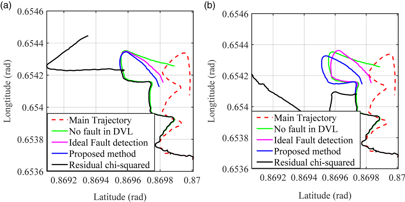
Figure 10. Test 2: Comparing navigation results for different fault-tolerance methods when DVL signals are available for (a) 70% and (b) 50% of the trajectory
Based on the results presented in Section 5.1, one can demonstrate that the suggested fault detection method detects the gradual fault of DVL signals, characterised in Table 2, 4 s earlier than the residual chi-squared test. According to the fact that the contaminated data is acquired until the detection moment and training phase of I-eTS structure is involved with the faulty data sets, the predictive ability of the INS/DVL decreases, which deviates the system from the intended navigation path (root mean square distance error increases by 18⋅59% for the residual chi-squared test in comparison with the proposed method). Moreover, in Figure 10(b), a similar scenario happens when 50% of the navigation path is followed (in this case, RMS distance error increases by 32⋅47%). In both cases, the navigation with the proposed FTS for INS/DVL integrated system reveals similar performance to the normal INS/DVL without any DVL malfunction. Nonetheless, as the navigation system gets further from the fault occurring moment, the integrated navigation system with residual chi-squared test tends to instability, but the proposed fault-tolerance method results in similar performance to the ideal integrated navigation system.
In Figure 11, the difference between DVL signals and INS output velocity signals, denoted by  ${\Delta }{V_{\textrm{DVL}}}$, is shown along each direction. The integrated navigation system with residual chi-squared test, in the fault occurrence interval, is unable to detect the fault quickly; consequently, the DVL estimator employs the contaminated data and loses the prediction ability. On the other hand, the FTS with the proposed fault detection method demonstrates acceptable performance in DVL signal prediction, with rapid fault detection. The performance of the proposed FTS for integration method is fairly close to the ideal integration navigation system. Such a desirable prediction makes the navigation system able to cope with the various DVL malfunctions and improves the stability of the I-eTS-based INS/DVL integrated system.

Figure 11. Test 2: Comparing prediction error of DVL signals between different fault tolerant methods: (a)  ${\Delta }{V_{DVL}}_x$, (b)
  ${\Delta }{V_{DVL}}_y$, (c)
  $\boldsymbol{\Delta }{V_{DVL}}_z$
6. Conclusion
A novel fault-tolerant AI-aided integration system was introduced in this paper for ocean navigation and applied to navigate under DVL malfunction conditions, with the results of performing real field tests of different manoeuvres. With a suggested fault detection method, due to the smooth fault detection function, lower thresholds were obtained compared with other well-known fault detection methods, that is, the residual chi-squared test. Two known types of faults were applied to the fault detection methods: gradual and abrupt faults. In the field test studies, it was demonstrated that the proposed fault detection method leads to rapid detection of gradual and abrupt faults. After fault detection occurs, the pseudo DVL signals are required to fulfil the role of DVL in the integrated navigation system. Having both proposed structures in cooperation, a FTS method emerged whose powerful capacity was demonstrated in analysis results. RMS distance error, an index to measure the precision of navigation, decreases by 18⋅59% for the proposed FTS method in comparison with the I-eTS in cooperation with residual chi-squared test. In other words, the interaction between fault detection and FTS with combination of GPR model and I-eTS is less than that for chi-squared and I-eTS.


