2. MECHANISM OF LIMS

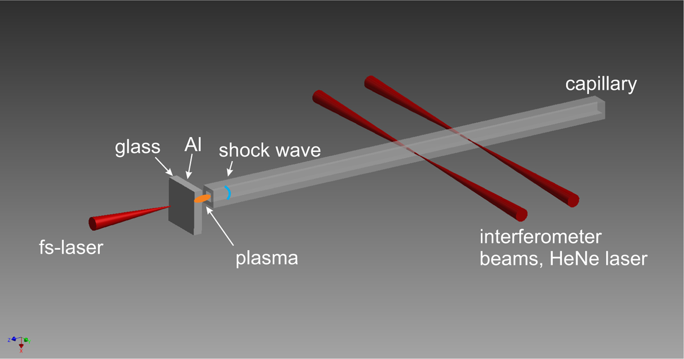
The working principle of LIMS is shown in Figure 1. A high power laser pulse is focused through a thin glass plate onto a thin aluminum (Al) layer evaporated on the rear side of the plate, where it generates almost instantaneously a laser-produced plasma (LPP). The sudden occurrence of a high-pressure, high-temperature LPP is an extreme non-equilibrium. To achieve the balance again, a shock wave as natural phenomenon is emitted. Thus, this LPP acts as a driver for the shock wave, which then propagates into a capillary positioned in the immediate vicinity.

Fig. 1. Illustration of the LIMS method. In reality the target (1 mm thick glass substrate with a 50 nm thin Al-layer) is in close vicinity ( $ \lt 5\, {\rm \mu} {\rm m}$ , but not in contact) to the capillary entrance, the sketch is exaggerated for clear viewing.

The LPP here is treated by a simple ‘δ-pulse model’, which can quite simply give a first estimate of the initial conditions of the LPP generated by an ultrashort laser pulse (Caruso & Gratton, Reference Caruso and Gratton1969; Teubner et al., Reference Teubner, Wülker, Theobald and Förster1995). The δ pulse model is a reasonable assumption, when the corresponding laser pulse duration τ_L is much shorter than the shock formation time τ_b. To achieve this, it is advantageous that τ_L is in the ps or fs range (later verified by the MULTI-fs simulation). The LPP acts as a homogenous quasi-planar driver for the shock wave, because the plasma is generated in the way that it is approximately of the same lateral diameter as the corresponding capillary.

For the present work, a Titanium: Saphire laser [linearly polarized, ${\rm \tau} _{\rm L} = 150 \,{\rm fs}$ (full-width at half-maximum (FWHM)], wavelength 775 nm, maximum pulse energy 1 mJ) is focused at normal incidence by a plano-convex lens with long focal length f. This yields a large focus, which is necessary for a lateral LPP that well fits to the capillary diameter. Experiments are performed with lenses of different f. The intensity I is always well beyond the plasma formation threshold of Al $(2 \times 10^{12}\, {\rm W}/{\rm cm}^2 )$ , but well below the ionization threshold of air $(5 \times 10^{14}\, {\rm W}/{\rm cm}^2 )$ and close to the optical breakdown in glass $(2 \times 10^{13}\, {\rm W}/{\rm cm}^2 )$ , respectively. All values given in brackets are deduced experimentally for conditions of the present work. Thus, plasma formation is mostly restricted to the thin Al-layer.

The target is shifted after each shot, so that the next laser pulse hits a fresh location on the target. Al layers (partly oxidized) of different thickness (between 30 and 100 nm) have been investigated, and the best suitable thickness is 50 nm. For the target with 50 nm Al layer, its absorption A = 65% is deduced from an independent measurement. From this A value, the initial penetration depth can be calculated as approximately 16.5 nm (but it changes during the laser–plasma interaction). Due to the oxidation, the penetration depth here is larger than that from pure Al [7.1–7.5 nm (Palik, Reference Palik1998)], but not too large, so that decent light absorption occurs.

Due to the fast non-linear heat wave within the thin Al layer, the LPP is nearly homogeneously heated and ionized. Thus the electron pressure P _e is approximately constant all over the LPP. For the typical value $I = 2 \times 10^{13}\, {\rm W}/{\rm cm}^2 $ of the laser pulse in this work, the initial electron temperature is several eV, the average ionization degree of the plasma is approximately 3 and thus the electron density is approximately $2 \times 10^{23}\, {\rm cm}^{ - 3} $ , which is hundred times the critical density. During the laser pulse itself, due to the large inertia, the electrons and ions are not in equilibrium. Only after a few ps both temperatures are equalized to a common temperature. Within a few ps, the LPP begins to expand significantly.

3. MULTIFS SIMULATION

A one-dimensional (1D) simulation using the MULTI-fs code (Ramis et al., Reference Ramis, Eidmann, Meyer-ter Vehn and Hüller2012) is performed to investigate the light–material interaction between the fs-laser pulse and the Al target. The secondary effect of this interaction is the generation of a shock wave, which also appears in this simulation. Note that, this 1D simulation is limited to the formation phase of the shock wave without the geometrical confinement enforced by the capillary. This is legitimate, because also in the experiments the capillary does not play a role yet in the very early stage of shock generation and propagation. Furthermore, due to the rather large focus and the rather thin LPP, the geometry can be regarded to be 1D until the shock wave is initiated. But later in time 2D effects become important and therefore the theoretical study of the subsequent shock propagation through the whole capillary requires two-dimensional (2D) Navier–Stokes computation (this is beyond the scope of the present work, which concentrates on the demonstration on a new method of micro shock generation).

MULTI-fs is a Lagrangian hydrodynamic code with multi-group radiation transport. It simulates the laser pulse propagation in the plasma region up to the critical surface by solving the wave equation, which results in a correct model of light reflection in plane geometry and thus provides realistic absorption values. Hence, the overestimation of the dynamic pressure by excessive absorption in the Al layer can be avoided.

The ions and electrons in the short-pulse-driven plasma may be far from thermodynamic equilibrium, and the code implies separate equation-of-state (EOS) tables for both species. The EOS data for Al are calculated with FEOS (Kemp & Meyerter Vehn, Reference Kemp and Meyer-ter Vehn1998; Faik et al., Reference Faik, Basko, Tauschwitz, Iosilevskiy and Maruhn2012) using the soft-sphere approximation (Young & Corey, Reference Young and Corey1995), which avoids overestimated plasma pressures in the two-phase region up to the critical point. The EOS tables are taken from SESAME library (T4GROUP, 1983; Lyon & Johnson, Reference Lyon and Johnson1992). The MULTI-fs simulation solves the equations for electron and ion internal energies. Pressure and temperature data are taken from the inverse EOS tables. The calculation of the evaluation of the transport processes in the plasma, the electron collision frequency, the electron thermal conduction and other quantities and also the consideration of opacity and radiation transport is described in more detail elsewhere (Teubner et al., Reference Teubner, Kai, Schlegel, Zeitoun and Garen2017).

Just as the experimental conditions, the MULTI-fs simulation uses the same set of laser parameters, namely: wavelength 775 nm, FWHM duration of 150 fs with a sin-squared intensity envelope, peak intensity $2 \times 10^{13}\, {\rm W}/{\rm cm}^2 $ . The transparent glass support for the 50 nm Al layer is mimicked by the boundary condition of zero flow velocity on the laser-illuminated Al boundary. The simulation shows 26% absorption of the laser energy in the Al layer. This result generally agrees with the experiment. Simulations also show that the electron number density is kept overcritical, which confirms the measured very low transparency. The final simulation results are the mass density, ion/electron pressure, ion/electron temperature, and flow velocity as functions of the shock propagation distance for different time instants. The most relevant values for this work are the mass density, ion pressure, and flow velocity.

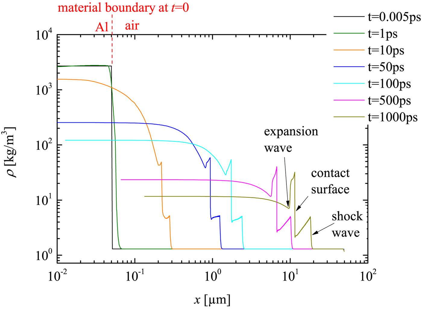
In Figure 2, the simulated mass density profiles of the target are displayed. t = 0 indicates the arrival time of the fs-laser pulse at the left boundary of the Al layer, thus this is approximately the initiation time of the plasma. The first edge from right side of the curve at t = 1 ns can be identified as the shock front and the edge just behind the contact surface. This observed flow profile is quite similar to that in a conventional shock tube, where the contact surface acts as a driving ‘piston’ behind the shock. But there is also difference to such tubes: the driver (namely the plasma) of LIMS is extremely short in space and highly transient. This can be seen from the ‘decreasing plateau’, that is, the decrease of the flow density immediately behind the shock front. It is important to remark that the contact surface only exists in the early stage, before the plasma recombination process finishes. This early stage is in the range of ns, and ends much before the temporal window of the experimental measurements, which is in the range of μs. Therefore one cannot expect to measure the contact surface in the experiment. Thus, the present simulations does provide information on the shock wave generation and the early phase of its propagation, which is not accessible by the measurement and in that sense it supplements the experimental work. Furthermore, it may be noted that the boundary layer development does not play an important role in the early phase and, of course, is not included in a 1D simulation. The expansion wave can also be identified in the density profile (Fig. 2). Moreover, the density behind the contact surface is also influenced by the temperature gradient. Thus, further statements about the expansion waves would need further analysis of the temperature (not shown here) and pressure profiles (see Fig. 3). But all this further analysis is not of much interest for the present work (namely the successful demonstration of a novel micro shock tube; for the same reason, the lack of experimental data in the early phase is not a drawback).

Fig. 2. MULTI-fs simulation of the density development of LIMS at initial stage (t from 0 to 1 ns). Different time steps correspond to different color.

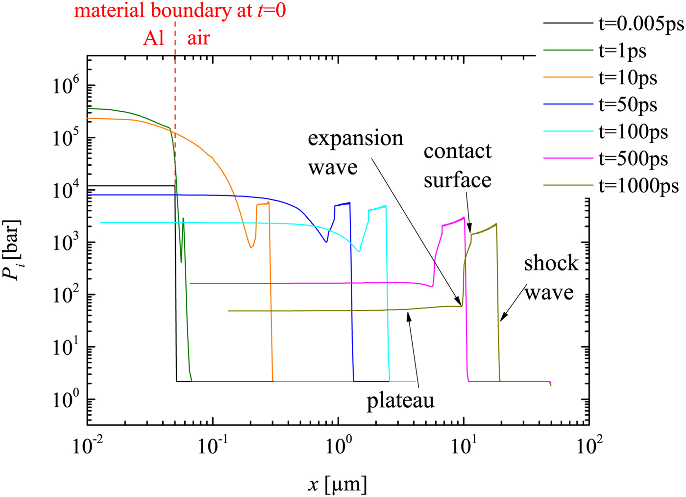
Fig. 3. MULTIfs simulation of the pressure development of the LIMS at initial stage.

The simulated ion pressure profiles are displayed in Figure 3. The electron pressure is also simulated but not shown here (it is an order of magnitude lower than the ion pressure after the shock wave sets off from the plasma into air after few ps of plasma initiation). Thus, the ion pressure is considered as the main driver of the shock. The pressure around the contact surface is much different from a typical conventional shock tube (e.g. Anderson, Reference Anderson2003), because here the pressure in front and behind the contact surface is not constant. This difference may be caused by the complicated plasma development (this is again just an additional observation but not of further relevance for the present work).

Here the contact surface corresponds to the first falling edge (from right, marked in Fig. 3), because in Figure 4 the trajectory of the first falling edge in the pressure profile overlaps with the trajectory of the second rising edge in the density profile (already known as the contact surface). The reflected expansion wave (moving from left to right) in the pressure profile corresponds also to the first negative peak from the left (again verified by Fig. 4). Further it is consistent with our expectation that the flow density and pressure behind the expansion (toward left hand side) will return to certain plateau value of the driver (marked as ‘plateau’ in Fig. 3).

Fig. 4. Wave diagram of the LIMS at initial stage, retrieved from the simulated data in Figures 2 and 3. ‘den. pro.’ is short for density profile, while ‘pres. pro.’ for pressure profile.

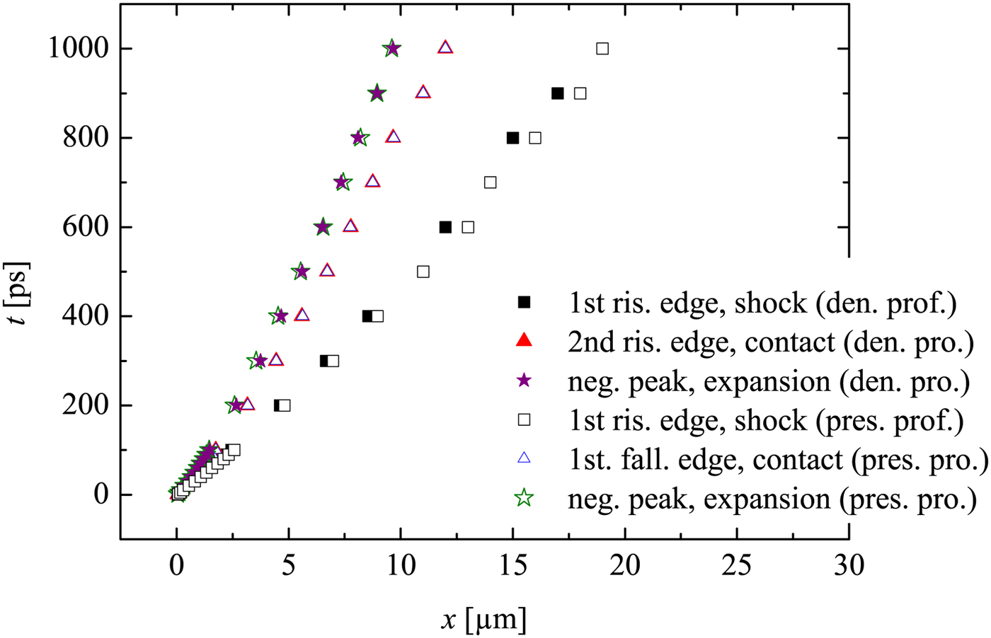
The wave diagram in Figure 4 provides important information on the flow trajectories. It is noticed that, the contact surface departs from the shock wave during the propagation. This is expected, because the driver density and the corresponding pressure decrease during the propagation, which are the results of the colder plasma due to recombination process and expanding volume. Note that the 2D dissipative effects are not included in the simulation, thus the contact surface deceleration due to wall friction is not considered here.

Figure 5 shows that the shock wave in air has a formation phase at the beginning, where shock acceleration occurs. This is similar to shock generation in conventional shock tubes. However, here the formation phase lasts dozens of ps only. Later on, the shock wave begins to attenuate. After 1 ns, the shock velocity is reduced to approximately half of its maximum value at the onset.

Fig. 5. Shock wave velocity development of the LIMS at initial stage. Retrieved from the MULTI-fs simulation data of the flow velocity.

At later time instants after plasma recombination, stronger attenuation is expected (not simulated here, due to limited computation power and time). Furthermore, there is limited quality of the applied EOS in the low-temperature range, which is different to standard laser–plasma simulation with higher intensity or long-term exposure. Nevertheless, the MULTI-fs simulation has provided important information for the initial conditions of LIMS.

4. EXPERIMENTAL SETUP

In the current experiments, a fs-laser is applied to generate an optical breakdown on a target, which is a 50 nm thin Al film on a glass substrate (Fig. 1). The experiments are performed with different commercially acquired glass capillaries (CM scientific) with hydraulic diameter of D = 50, 100, and 200 µm, respectively. The capillary wall is half the thickness of the hydraulic diameter of the capillary.

The shock wave propagation in the capillary is investigated by a laser differential interferometer (LDI), which is a modification of the arrangement in Udagawa et al., (Reference Udagawa, Garen, Meyerer and Maeno2007) and Kai et al., (Reference Kai, Garen and Teubner2017). To ensure a precise alignment, two self-made microscopes with cameras are applied to provide top and front views of the capillary and LDI alignment. This also allows exact target positioning using motorized stages.

At the detection plane, the interferometric beams are measured by two corresponding photodiodes (rise time 10 ns) connected to an oscilloscope. When a shock wave propagates through one of the LDI beams, a signal is generated. The time delay between the two signals from the two LDI beams is Δt, which can be read from the temporal signal of the oscillograph. The distance Δx between the LDI beams is preset to 370 µm. Thus, the time-of-flight method provides the shock wave velocity, which is simply given by u _s = Δx/Δt.

For the measurement of the shock wave propagation at different distances x (the target is located at x = 0), the LDI is shifted at the corresponding position. For every x the measurements are reproduced five times (at critical points, ten times). Within the present work, the measured shock trajectory is fitted by an allometric function x(t) = a·t ^b that consists only of the parameters a and b. Since the direct differentiation of experimental data leads to large uncertainties, it is quite common to represent the experimental data by an appropriate fit function prior to further processing. The derivative of the fit function x(t) also provides the shock wave velocity u _s, which well agrees with the direct time-of-flight method, but has a higher resolution [see Teubner et al., (Reference Teubner, Kai, Schlegel, Zeitoun and Garen2017)].

Applying basic knowledge in optics, one can derive the density of the flow from the amplitude signal given by the photo diodes (also read from the oscillograph):

(1) $$\displaystyle{{{\rm \rho} (t)} \over {{\rm \rho} _1}} = a{\rm sin}\left( {\displaystyle{{U(t)} \over {U_0}}} \right) \displaystyle{{\rm \lambda} \over {2\pi {\rm \kappa} D}}\displaystyle{{P_N} \over {P_1}} + 1, $$

where κ is the Gladstone-dale constant (for air at the normal conditions κ = 2.83 × 10⁻⁴), ρ is the flow density, and P is the pressure. Index 1 indicates the state in front of the shock. U ₀ is the maximum photo voltage. U(t) is the voltage signal. Note that, this equation is valid before the shock wave arrives at the second interferometric beam.

5. EXPERIMENTAL RESULTS

5.1. Shock Wave Propagation

Figure 6 is the wave diagram of the shock waves. The diagram clearly shows that shock waves generated with the same laser intensity in larger capillaries propagate faster than those in smaller capillaries. As expected, due to the dissipative effects, the shock wave in all capillaries attenuates to sound velocity (straight dash lines in the diagram). The positions where shocks become sound waves are $x_{{\rm sw}} = 1888\, {\rm \mu} {\rm m}$ , $x_{{\rm sw}} = 2707\, {\rm \mu} {\rm m}$ , and $x_{{\rm sw}} = 7913\, {\rm \mu} {\rm m}$ for the capillaries with diameters 50, 100 and 200 µm, respectively. This shows stronger attenuation (due to wall friction) for smaller capillaries [a detailed discussion may be found elsewhere (Teubner et al., Reference Teubner, Kai, Schlegel, Zeitoun and Garen2017].

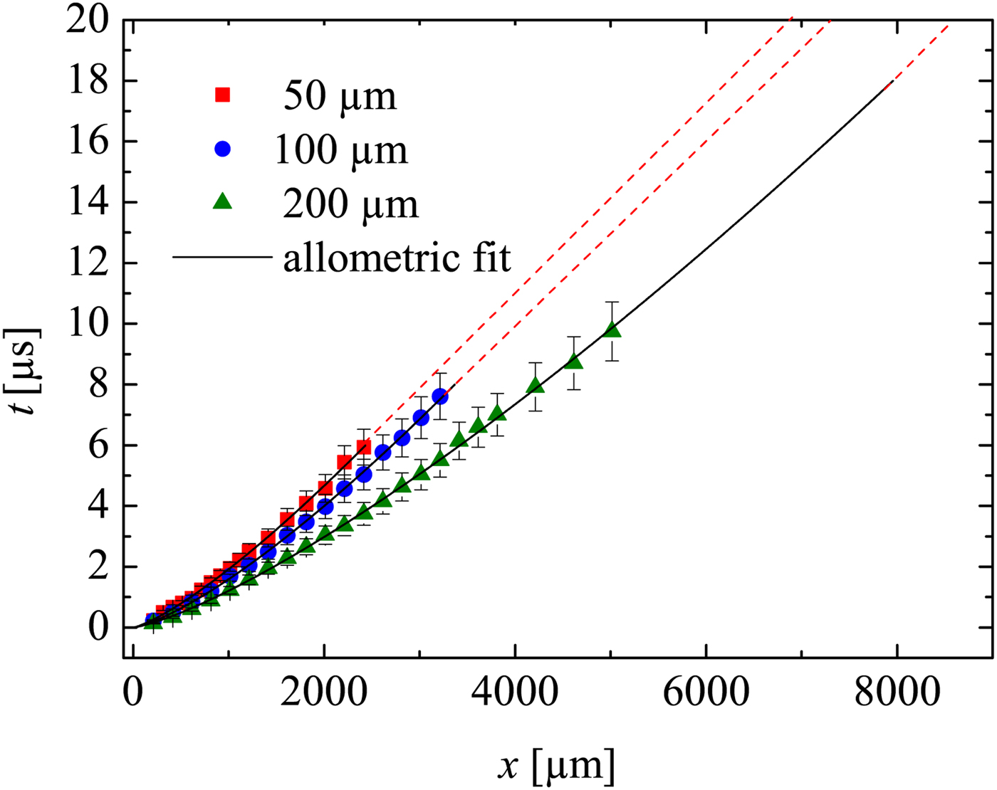
Fig. 6. Shock wave ‘t–x’ diagram determined by LDI. Straight dash lines indicates sound wave propagation. The laser intensity is the same for all experiments. Extrapolation of the 200 µm capillary is made till sound wave propagation.

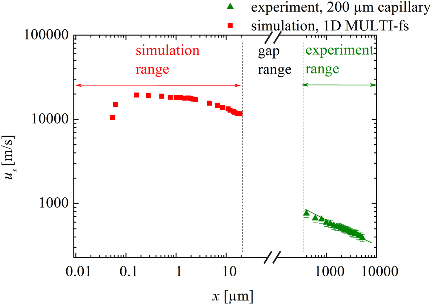
As an example, Figure 7 shows the shock velocity attenuation data for the 200 µm capillary obtained from the experiments. In addition and for comparison, the simulated u _s(x) data discussed in Section 3 are plotted here again. The experimental data and those obtained from the simulation are obviously separated by a gap ( $20\, {\rm \mu} {\rm m} \lt x \lt 215\, {\rm \mu} {\rm m}$ ). The reason for this is that the experimental setup allows far-field measurements only (fully developed shock), whereas the hydrocode simulation is restricted to the near field (plasma generation and shock formation). Although there is no overlap between simulation and experiment (investigation of this overlap region may be subject of the future), it does not affect the present work that concentrates on the demonstration of a novel method for micro shock generation in small capillaries. The present work clearly shows the initiation of the shock wave close to the entrance of a capillary. This is modeled successfully in the ‘near-field region’. Even though data are missing in the gap region, the experimental observations verify the propagation of rather strong shock waves in the ‘far-field region’. Nonetheless the transition of the shock velocity values from the near field to the far-field region may be discussed qualitatively. As discussed above, initially the LPP can be regarded as a quasi-planar driver which generates a rather planar shock wave. After a couple of micrometers (this is also the distance when the shock enters the capillary), propagation is restricted and wall friction and heat conduction are expected to occur. However, these effects are not included in the 1D hydrocode simulations, thus the attenuation is considerably underestimated, and the shock velocity overestimated [it may be noted that the underestimation of the attenuation is even more pronounced for the smaller capillaries (not shown here)]. Furthermore, the LPP driver is not present anymore (the typical lifetime of the plasma is between 10 and 100 ps). As a result the LPP stops driving the shock in this gap range, causing the shock strength to suddenly decrease. Subsequently, the shock in the far field begins with a much reduced value of u _s, which is indeed the observation within the experiments (see, e.g., value at $x = 200\, {\rm \mu} {\rm m}$ ).

Fig. 7. Shock wave velocity attenuation. Simulated data replotted from Figure 5. Experimental data determined by (1) the time-of-flight method (scattered points with 10% error bars). and (2) the derivative of the fit of the trajectory (solid lines). The laser intensity is the same for all experiments.

In Figure 8, the development of the density jump ρ₂/ρ₁ across the shock is displayed. For x/D < 10 (i.e. $x \lt 500\, {\rm \mu} {\rm m}$ ), the shock wave may not yet have a full planar geometry. This is supported by Figure 9, because the first rising edge is not really sharp (the LDI beams ‘see’ through a bend instead of a flat surface of the shock wave). That indicates that ρ₂/ρ₁ is not measured correctly by the LDI (this shows the limitations for near-field measurements). However, further away (x/D > 10) the shock wave becomes more planar. Hence, ρ₂/ρ₁ is then measured properly and approximately agrees with Rankine–Hugoniot relations (with about 10% error). Furthermore, a density drop shortly behind the shock wave is well seen in Figure 9 for the curves x = 600 and $1000 \,{\rm \mu} {\rm m}$ . This effect may be caused by the unsteady driver and the expansion wave, which initially propagated toward the bottom of the capillary, then got reflected from the target plane, further followed the shock wave propagating in the same direction. This experimental observation supports the Navier–Stokes computations in Teubner et al., (Reference Teubner, Kai, Schlegel, Zeitoun and Garen2017).

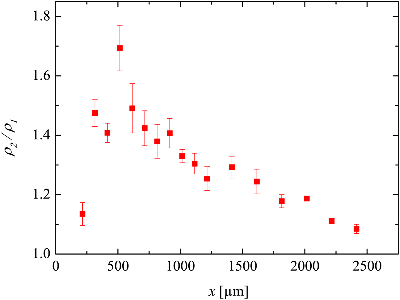
Fig. 8. The development of the density jump across the shock in the 50 µm capillary. The error bars here correspond to the standard deviation resulted from the shot-to-shot errors.

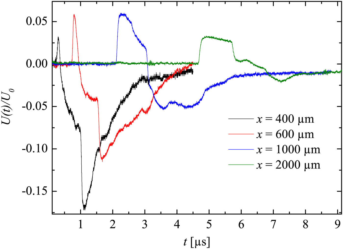
Fig. 9. The normalized oscillograms corresponding to the shock detections in the 50 µm capillary.

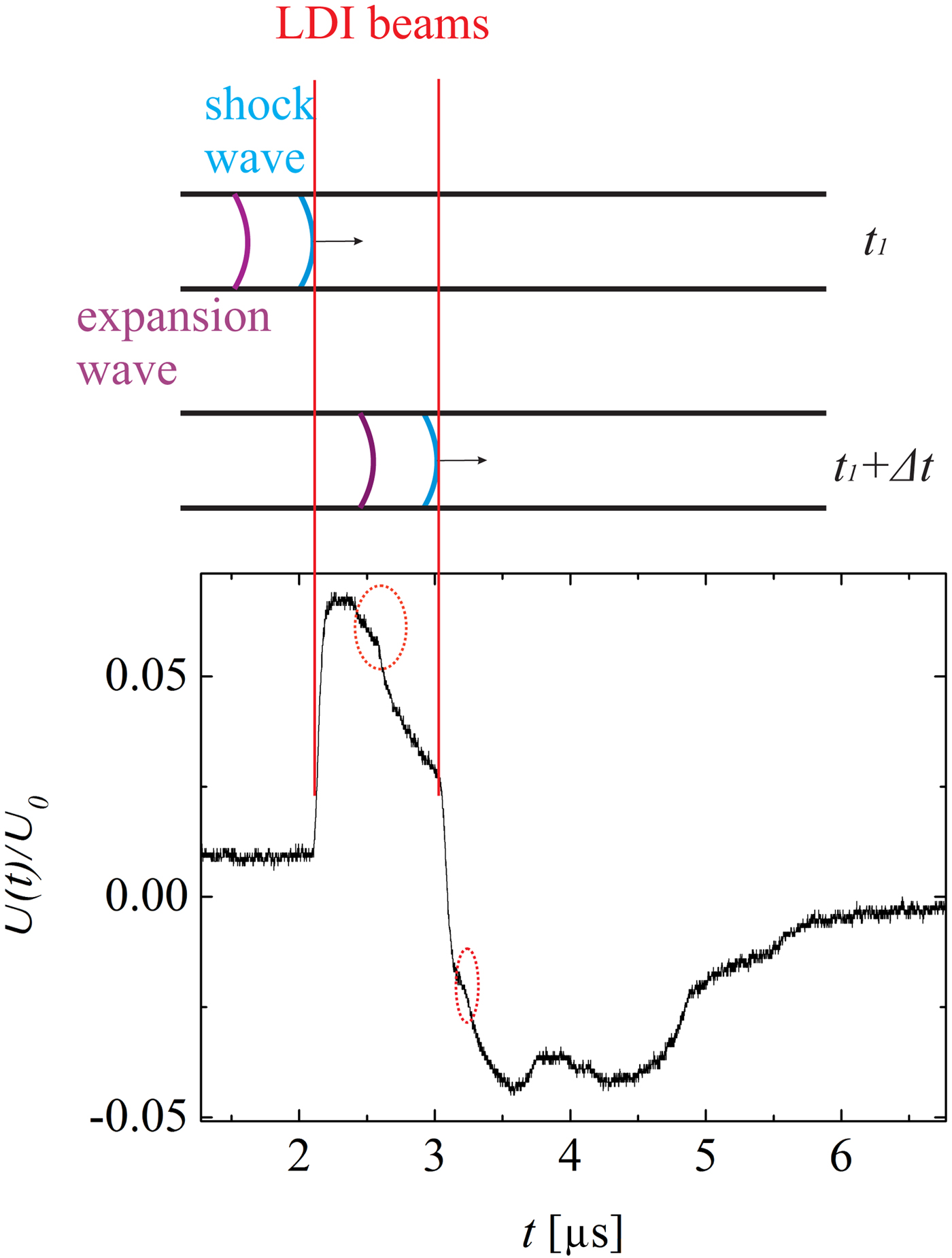
A detailed view of the detection of the shock wave and the expansion wave is shown in Figure 10. Due to the shock wave induced sudden density jump, the shock wave leads to sharp rising and falling edges in the oscillograms. This curve also shows the expansion wave (inside the dotted circles), which causes relatively gentle density changes. Moreover, it can be recognized that fairly soon after the shock wave reaches the first LDI beam (but before it reaches the second one), the expansion wave also reaches the first LDI beam. As an example, in the situation illustrated Figure 10, the expansion wave closely follows the shock wave, so that the density/pressure drops immediately after the shock wave passed by the first LDI beam. On the other hand, measurements carried out at larger distances x show that the expansion wave lags further behind the shock wave ( $x = 2000 \,{\rm \mu} {\rm m}$ in Fig. 9). In this case, after the wave shock has already passed both the LDI beams, the expansion wave reaches the first LDI beam.

Fig. 10. Illustration of the detection of a shock wave using the LDI. The oscillograph is taken at $x = 1000 \,{\rm \mu} {\rm m}$ in the 50 µm capillary. The sharp rising and falling edges are caused by the shock wave. The dotted circles highlight the expansion wave signal.

5.2. Shock-Induced Mass Motion and Reynolds Number

A shock wave is a pressure wave with supersonic velocity. The shock wave itself is not mass transport but a propagation of vibration. However, due to its supersonic nature, the gas molecules behind the shock wave are pulled into motion by the shock wave. Therefore, mass transport can be induced by a shock wave.

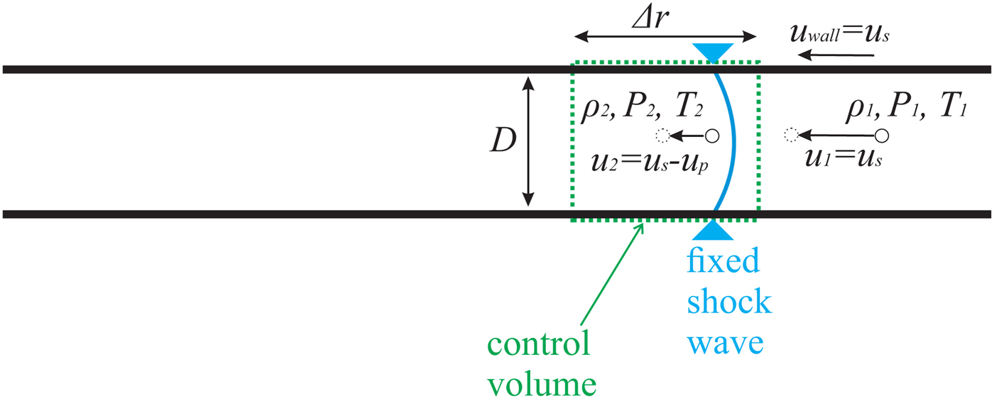
An illustration of shock wave propagation is shown in Figure 11. Instead of a laboratory reference frame, here a shock-fixed reference frame is applied, so that the continuity equation can be used for control volume analysis. Following Anderson (Reference Anderson2003), then the mass motion u _p can be determined by inserting the measured u _s and ρ₂/ρ₁ into the continuity equation

(2) $$(u_{\rm s} - u_{\rm p} ){\rm \rho} _2 = u_{\rm s} {\rm \rho} _1, $$

where ${\rm \rho} _1 = 1.177\, {\rm kg}/{\rm m}^3 $ at 300 K temperature [online data bank (2016)]. The right-hand side of the equation describes the entrance of the control volume, the left-hand side the exit.

Fig. 11. Illustration of gas propagating through a stagnate shock wave in a capillary. The shock-fixed reference frame is applied.

The ratio ρ₂/ρ₁ can be obtained from the Rankine–Hugoniot relation for the fluid density ratio across the shock wave

(3) $$\displaystyle{{{\rm \rho} _2} \over {{\rm \rho} _1}} = \displaystyle{{({\rm \gamma} + 1)M_1^2} \over {2 + ({\rm \gamma} - 1)M_1^2}}, $$

γ is the specific heat ratio, which is 1.4 for air.

The combination of Eqs. 2 and 3 yields an equation for the calculation of the mass motion u _p

(4) $$u_{\rm p} = u_{\rm s}\left( {1 - \displaystyle{{{\rm \rho} _1} \over {{\rm \rho} _2}}} \right) = {M_1}u_{\rm a}\left( {1 - \displaystyle{{2 + ({\rm \gamma} - 1)M_1^2 } \over {({\rm \gamma} + 1)M_1^2 }}} \right). $$

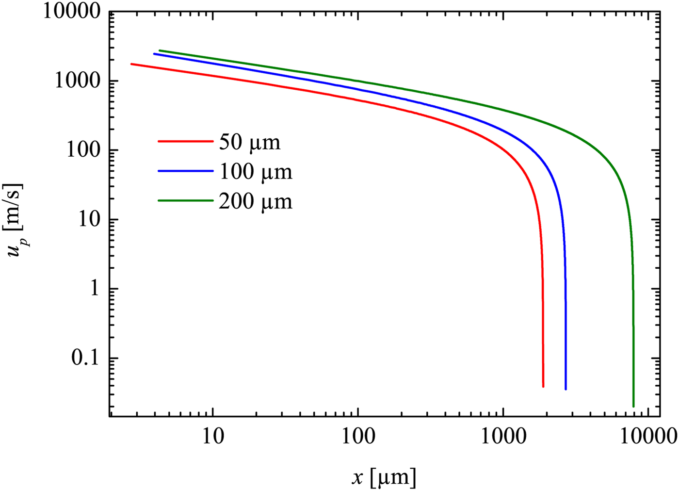
Inserting M ₁ (x) (deduced from M ₁ = u _s/u _a, with u _a as sound velocity) into Eq. 4. it yields u _p as a function of x (see Fig. 12).

Fig. 12. Velocity of the shock induced mass motion plotted against the propagation distance. Derived from the trajectory fit.

In the early stage of the measurement range, u _p can be as high as 500 m/s for the 200 µm capillary, 400 m/s for the 100 µm capillary and approximately 230 m/s for the 50 µm capillary.

With the knowledge of u _p, it is possible to derive the Reynolds number for the flow. This is helpful for the analysis of the flow behavior immediately behind the propagating shock wave. Due to the large particle velocity u _p behind the shock, the mainstream flow is turbulent in conventional shock tubes with large diameters. However, the situation can change with extremely thin tubes and/or with very dilute gases, so that the flow behind the shock becomes laminar. This is indicated by the Reynolds number Re ₂ (Sun et al., Reference Sun, Ogawa and Takayama2001; Garen et al., Reference Garen, Meyerer, Udagawa and Maeno2009):

(5) $$Re_2 = u_{\rm p} D{\rm \rho} _2 /{\rm \mu} _2. $$

Here it should be remarked that the definition of a Reynolds number Re ₂ may not always be useful, if this definition is with respect to a location x where a significant boundary layer is present. However, here we define Re ₂ closely behind the shock wave where boundary layer effects can be ignored. Thus Re ₂ can be regarded as a useful quantity.

Since for small to moderate Mach numbers the dynamic viscosity does not depend on temperature and pressure, μ₂ can be replaced by the known viscosity μ₁=1.85·10⁻⁵ kg/(m·s) (ambient air at room temperature 300 K) [online data bank (2016)]. From the combination of Eqs. (2)–(5), one obtains:

(6) $$Re_2 = \displaystyle{{u_{\rm s} D{\rm \rho} _1} \over{{\rm \mu} _1}} \left( {\displaystyle{{({\rm \gamma} + 1)M_1^2} \over {2 + ({\rm \gamma} -1)M_1^2}} - 1} \right),$$

which can be simplified as

(7) $$Re_2 = Re_0 M_1 \displaystyle{{M_1^2 - 1} \over {0.2M_1^2 + 1}}.$$

Here Re ₀ = γ ₁ Dp ₁/(u _a μ₁), where γ ₁ is the adiabatic exponent. Re ₂ therefore only depends on the variable M ₁. As a result, a measurement of the time-dependent Mach number M ₁(t) yields the time-dependent Reynolds number Re ₂(t). This is shown in Figure 13. It can be well seen that the flow behind the shock wave is turbulent for short periods only. In particular, for quite small capillaries, the laminar region is reached rather quickly; whereas in larger capillaries, the shock propagates significantly longer (both, in space and time) in the turbulent regime. Nevertheless, at long enough x or t, the flow becomes always laminar for all capillaries. This is different with macroscopic tubes, where the propagation is nearly always in the turbulent regime.

Fig. 13. The Reynolds number Re ₂ closely behind the shock front as a function of the normalized propagation time (t _sw is the time, when the shock wave has slowed down to sound wave velocity; see the last section).