


1. Introduction
It is of importance to understand and predict the transition process in the boundary layers over turbine blades, as it largely determines the load and heat transfer on the blade, and the overall efficiency of the turbine (Mayle Reference Mayle1991; Jahanmiri Reference Jahanmiri2011). The key factors affecting instability and transition include high turbulence level, pressure gradient and surface curvature (Volino & Simon Reference Volino and Simon1995, Reference Volino and Simon2000; Schultz & Volino Reference Schultz and Volino2003). Since the pressure gradient is favourable in an extended region from the leading edge, the flow there remains laminar, but exhibits strong three-dimensional and unsteady characteristics due to the influence of free stream turbulence (FST) and centrifugal force. In the case of a concave wall, Görtler instability operates to cause earlier transition, the extent of which depends on the levels of FST, but a convex curvature has little effect at all turbulence levels (Kim, Simon & Russ Reference Kim, Simon and Russ1992; Volino & Simon Reference Volino and Simon1995, Reference Volino and Simon1997). Currently, transition location is determined by using empirical correlations deduced from limited experimental data (Walker Reference Walker1993). In the case of flat-plate boundary layer, several relations between the transition Reynolds number and FST level have been proposed with or without a pressure gradient (Abu-Ghannam & Shaw Reference Abu-Ghannam and Shaw1980; Gostelow, Blunden & Walker Reference Gostelow, Blunden and Walker1994). However, the role of the spectra or length scales of FST has not been quantified despite the fact that they were found to be also relevant (Volino & Simon Reference Volino and Simon1995), and neither have the combined effects of the pressure gradient nor the curvature been accounted for. Better understanding of the transition process is crucial for the development of a physics-based transition prediction method. In this paper, we investigate the fundamental process of transition in the boundary layer over a flat or concave wall subject to a pressure gradient. Specifically, the generation of Görtler vortices by free stream vortical disturbances (FSVD) and their evolution and secondary instability are to be considered in a unified framework, in which the pressure gradient, FSVD and curvature are all taken into account.
1.1. Görtler vortices
Görtler instability occurs in a boundary layer over a concave wall due to the imbalance between the centrifugal force and the wall-normal pressure gradient. Görtler (Reference Görtler1941) started the investigation of this instability using a local normal-mode approach based on a parallel-flow approximation. The key parameter controlling the instability was identified to be the Görtler number, defined as  $G_\theta =(U_\infty \theta /\nu )\sqrt {\theta /r_0^{*}},$ where
  $U_\infty$ is the free stream velocity,
  $\theta$ and
  $r_0^{*}$ denote the boundary layer (momentum) thickness and radius of curvature, respectively, and
  $\nu$ the kinematic viscosity. The instability causes the formation of spanwise-periodic and streamwise-elongated vortices. The analysis of Görtler was extended by Smith (Reference Smith1955), Ragab & Nayfeh (Reference Ragab and Nayfeh1980) and Floryan & Saric (Reference Floryan and Saric1982), who sought to include part of the non-parallel-flow effects, but continued to treat the instability as an eigenvalue problem. These studies showed that Görtler vortices with a fixed wavelength decay near the leading edge, but start to amplify from some distance downstream. However, without fully accounting for the streamwise variation of both the base flow and modal shape, the growth rate predicted by the local theory is unsatisfactory in comparison with experimental results (Tani Reference Tani1962; Finnis & Brown Reference Finnis and Brown1997).
Hall (Reference Hall1982, Reference Hall1983) was the first to point out that in the general case where  $G_\theta =O(1),$ Görtler instability should be formulated as an initial value problem, which has to be solved by using a marching method. A local approach is justified only in the limit of
  $G_\theta \gg 1,$ or equivalently sufficiently downstream for vortices with a fixed wavelength. The distinguished local instability regimes in the limit
  $G_\theta \gg 1$, for which the spanwise wavelength of the vortices is much shorter than the local boundary layer thickness, were identified by Hall (Reference Hall1982) and Denier, Hall & Seddougui (Reference Denier, Hall and Seddougui1991). Hall (Reference Hall1983) solved the linear initial value problem and showed that different initial (upstream) conditions led to different transient behaviour, and only at large distances downstream do the vortices become neutral in the same manner as was described by the large-
 $G_\theta$ asymptotic theory (Hall Reference Hall1982). These theoretical findings were reconfirmed by numerical studies of Day, Herbert & Saric (Reference Day, Herbert and Saric1990), Goulpié, Klingmann & Bottaro (Reference Goulpié, Klingmann and Bottaro1996) and Bottaro & Luchini (Reference Bottaro and Luchini1999), who solved the local stability problem at finite
  $G_\theta$. The predicted growth rate was compared with that by the marching method, and the two was found to overlap only sufficiently far downstream. The nonlinear initial value problem was first formulated and solved numerically by Hall (Reference Hall1988), and his calculations showed that nonlinear development of Görtler vortices depends on the upstream condition in general, but may reach a ‘local equilibrium state’ if the surface curvature increases sufficiently rapidly with the distance.
Theoretical analyses (Hall Reference Hall1983, Reference Hall1988) and experiments (Swearingen & Blackwelder Reference Swearingen and Blackwelder1987; Kottke Reference Kottke, Westifield and Brand1988) indicate that the initial condition is vital for describing the evolution of Görtler vortices. For this reason, receptivity, i.e. the process of generating vortices by external disturbances, should be treated as an integrated part of the Görtler instability theory. Surface roughness elements and free stream turbulence are two main relevant external disturbances. Denier et al. (Reference Denier, Hall and Seddougui1991), Bassom & Hall (Reference Bassom and Hall1994) and Sescu & Thompson (Reference Sescu and Thompson2015) studied the generation of Görtler vortices by roughness. They found that the shape and size (height and diameter) of roughness elements influence the excitation and evolution of the vortices. Sescu & Afsar (Reference Sescu and Afsar2018) studied wall deformations to hamper the Görtler vortices excited by roughness using an optimal control method.
How free stream turbulence excites precisely Görtler vortices and streak-like disturbances in the boundary layer is a topic of intense recent interest. Direct numerical simulations (DNS) were performed by Schrader, Brandt & Zaki (Reference Schrader, Brandt and Zaki2011). In their work, the FSVD and inlet disturbances are represented by the continuous modes of the Orr–Sommerfeld (O–S) and Squire operators, in which non-parallelism is neglected completely. Unfortunately, these continuous modes are non-physical, and their eigenfunctions do not represent entrainment of FSVD into the boundary layer because the latter is fundamentally influenced by non-parallel-flow effects, as was pointed out by Dong & Wu (Reference Dong and Wu2013). For the flat-plate boundary layer, Leib, Wundrow & Goldstein (Reference Leib, Wundrow and Goldstein1999) showed that long-wavelength, low-frequency FSVD induce streaks, which are governed by linear unsteady boundary region equations. Ricco, Luo & Wu (Reference Ricco, Luo and Wu2011) extended their work to the case where FSVD are strong enough to generate nonlinear streaks. Generation of linear and nonlinear streaks in a compressible boundary layer has been considered by Ricco & Wu (Reference Ricco and Wu2007) and Marensi, Ricco & Wu (Reference Marensi, Ricco and Wu2017), respectively. On the other hand, Wu, Zhao & Luo (Reference Wu, Zhao and Luo2011) extended the work of Leib et al. (Reference Leib, Wundrow and Goldstein1999) to a concave wall and studied the excitation of Görtler vortices by FSVD and their linear evolution. Xu, Zhang & Wu (Reference Xu, Zhang and Wu2017) (referred to as Reference Xu, Zhang and WuXZW hereafter) furthermore investigated the nonlinear evolution and secondary instability of Görtler vortices induced by FSVD, and obtained results in good agreement with experimental measurements. This theoretical work presented a self-consistent framework to connect, on the basis of first principles, the characteristics of FST with the transition process. Borodulin et al. (Reference Borodulin, Ivanov, Kachanov and Mischenko2018) carried out the first detailed study of the excitation of Görtler vortices using controlled FSVD.
1.2. The influence of pressure gradient
A strong streamwise pressure gradient always exists in turbomachinery, and indeed influences the onset of transition (Schreiber, Steinert & Küsters Reference Schreiber, Steinert and Küsters2002). However, previous studies of pressure-gradient effects have mostly restricted to (a) streak formation and bypass transition in boundary layers over flat walls and (b) linear Görtler instability using the Falkner–Skan solutions as a model flow.
Experimental studies of bypass transition in the flat-plate boundary layer showed that, when in the presence of a streamwise acceleration the transition onset location shifted downstream (Blair Reference Blair1992; Talamelli, Fornaciari & Westin Reference Talamelli, Fornaciari and Westin2002) and became dependent on the history of the pressure gradient, as a result of which correlating it with a local pressure gradient parameter is inadequate (Abu-Ghannam & Shaw Reference Abu-Ghannam and Shaw1980; Solomon, Walker & Gostelow Reference Solomon, Walker and Gostelow1996). Zaki & Durbin (Reference Zaki and Durbin2006) performed DNS of transition triggered by the continuous modes, which were presumed to represent FSVD (but see Dong & Wu (Reference Dong and Wu2013), who pointed out the problems with this presumption). With the base flow being taken to be the Falkner–Skan boundary layer, an adverse pressure gradient enhanced streaks and as a result transition occurred earlier. Johnson & Pinarbasi (Reference Johnson and Pinarbasi2014) calculated the linear response to continuous modes. The streaks in the presence of an adverse pressure gradient were found to be stronger than those in the favourable pressure gradient case. Brinkerhoff & Yaras (Reference Brinkerhoff and Yaras2015) conducted DNS of bypass transition in a boundary layer subjected to an adverse pressure gradient and elevated FST. They pointed out that two distinct processes, the development of varicose secondary instability and a rapid amplification of free stream disturbances in the inflectional boundary layer, caused rapid transition to turbulence.
For a Falkner–Skan boundary layer, the local linear stability analysis of Ragab & Nayfeh (Reference Ragab and Nayfeh1980) indicates that an adverse pressure gradient is destabilising. This conclusion was confirmed by the marching method calculations with the upstream condition being taken to be an eigenmode or a more or less arbitrary disturbance velocity distribution (Goulpié et al. Reference Goulpié, Klingmann and Bottaro1996; Matsson Reference Matsson2008). Rogenski, de Souza & Floryan (Reference Rogenski, de Souza and Floryan2016) performed simulations using the linearised Navier–Stokes (N–S) equations, which require an artificial ‘buffer region’. Spanwise periodic suction/blowing was introduced to excite Görtler vortices, and different forms of pressure gradient were considered. For all the cases, the destabilising/stabilising effect of an adverse/favourable pressure gradient were observed again, but the variation of pressure gradient had a small effect once the vortices were established. Further calculations including nonlinearity showed that an adverse pressure leads to earlier saturation and higher saturated amplitude (Rogenski et al. Reference Rogenski, de Souza and Floryan2016). To the best of our knowledge, no existing work has considered the receptivity of streaks or Görtler vortices to physically realisable FSVD in the presence of a pressure gradient despite the experimental evidence indicating clearly that FSVD excite Görtler vortices (Aihara& Sonoda Reference Aihara and Sonoda1981; Kim et al. Reference Kim, Simon and Russ1992; Volino & Simon Reference Volino and Simon1995). It should be pointed out that although a Falkner–Skan solution may, with a suitably chosen Hartree parameter, be used as a proxy of a local profile of a boundary layer with a streamwise pressure gradient, it neither represents nor approximates any boundary layer globally because its far-field velocity is unbounded at upstream infinity, different from the uniform and bounded far-field of a typical flow past an aerodynamic body. It is impossible to specify physically meaningful disturbances in the oncoming flow, and thus a Falkner–Skan solution cannot be a useful vehicle for studying receptivity. Moreover, unless the Görtler number is large, it is not well-suited for analysing linear Görtler instability because vortices have a long scale, and are dependent on the entire base flow.
1.3. Secondary instability
Nonlinear Görtler vortices cause strong distortions of the streamwise velocity profile in both the wall-normal and spanwise directions (Hall Reference Hall1988; Lee & Liu Reference Lee and Liu1992; Benmalek& Saric Reference Benmalek and Saric1994). The resulting inflectional velocity profile may be highly unstable to high-frequency disturbances, which is referred to as secondary instability. The secondary instability of Görtler vortices in the zero-pressure-gradient boundary layer was first formulated and analysed by Hall & Horseman (Reference Hall and Horseman1991), and further information was provided by subsequent studies (Yu & Liu Reference Yu and Liu1994; Li & Malik; Reference Li and Malik1995; Reference Xu, Zhang and WuXZW). The only study of pressure-gradient effect on secondary instability of Görtler vortices is that of Aihara & Sonoda (Reference Aihara and Sonoda1981), which attributed the effect to a change of the high shear layer where secondary modes are amplified. The majority of experimental work focused primarily on correlating the transition location with the FST intensity on an empirical basis (Blair Reference Blair1982). The influence of pressure gradient on the secondary instability of Görtler vortices remains to be investigated.
1.4. The aim of current work
In the present paper, we will study streaks and Görtler vortices in a boundary layer subject to a streamwise pressure gradient, covering the aspects of excitation by high-intensity FSVD, nonlinear evolution and secondary instability of the vortices induced. The flow in real gas turbines is highly compressible, but incompressibility will be assumed in order to focus on the pressure-gradient effect. To retain the key physics while keeping the problem mathematically tractable, we consider the boundary layer over a flat or curved plate inserted into a contracting or expanding channel. This setting is analogous to the use of a contoured ceiling to create a pressure gradient. In § 2, we formulate the problem by describing the vortical disturbances in the oncoming flow and specifying the scaling relations. The flow is governed by an asymptotic structure consisting of four zones as is illustrated in figure 1. Two of those, referred to as regions I and IV, are outside the boundary layer and at distances  $O(\Lambda )$ and
  $O(\Lambda R_{\Lambda })$ to the leading edge, respectively, where
  $R_\Lambda$ is the Reynolds number based on
  $\Lambda$. Different from the zero-pressure-gradient case, the inviscid base flow is now non-uniform. As a result, the vortical disturbances undergo distortion. The disturbances in these two regions are analysed to provide the appropriate boundary conditions. The response in region II, i.e. the boundary layer underneath regionI, is obtained to provide the initial condition for the NBRE that govern the vortices induced in region III, the boundary layer underneath region IV. In § 3, the numerical procedure to solve NBRE is presented. Numerical results are presented in § 4. The secondary instability of the induced Görtler vortices is analysed in § 5. Finally, a summary and conclusions are given in § 6.

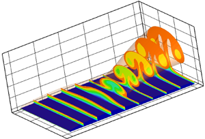
Figure 1. Schematic illustration of the physical problem and the associated asymptotic structure.
2. Formulation
We consider the incompressible boundary layer flow over a concave plate with a characteristic radius of curvature  $r_0^{*}$. The plate is placed in the middle of a contracting or expanding stream between two contoured ceilings, which are often used to induce a pressure gradient in experiments (Abu-Ghannam & Shaw Reference Abu-Ghannam and Shaw1980; Gostelow et al. Reference Gostelow, Blunden and Walker1994). Theceilings far upstream and downstream of the contracting/expanding sector are parallel so that the oncoming flow is uniform with a speed
  $U_\infty,$ superimposed on which is stationary, homogeneous turbulence. The flow is described in a curvilinear system
  $\boldsymbol {x}=(x_1,x_2,x_3)=x\skew3\hat {\boldsymbol {i}} +y\skew3\hat {\boldsymbol {j}}+z\skew3\hat {\boldsymbol {k}},$ normalised by the spanwise integral scale of the turbulence,
  $\Lambda$, with
  $x$ and
  $y$ being along and normal to the plate, respectively, and
  $z$ along the span. The dimensionless time
  $t$ and velocity
  $\boldsymbol {u}$ are introduced by using the reference time
  $\Lambda /U_\infty$ and velocity
  $U_\infty$, respectively. On assuming that the oncoming mean flow is uniform with the velocity field
  $(1,0,0)$, and the superimposed free stream turbulence consists of small-amplitude vortical fluctuations, the upstream velocity field can be written as
 \begin{equation} \boldsymbol{u}= (1,0,0)+\epsilon \boldsymbol{u}_\infty(x-t,y,z), \end{equation}
where  $\epsilon \ll 1$ is a measure of the disturbance intensity. The Reynolds number based on
  $\Lambda$ is defined as
 \begin{equation} R_\Lambda=U_\infty \Lambda/\nu, \end{equation}
where  $\nu$ is the kinematic viscosity. Furthermore, the turbulent Reynolds number,
 \begin{equation} r_t=\epsilon R_\Lambda \end{equation}
is introduced. The global Görtler number  $G_\Lambda$ is defined as (Wu et al. Reference Wu, Zhao and Luo2011)
 \begin{equation} G_{\Lambda}=R_{\Lambda }^{2}\Lambda /r_{0}^{*}. \end{equation}
The Reynolds number  $R_\Lambda$ is assumed asymptotically large, i.e.
  $R_\Lambda \gg 1,$ but the Görtler number
  $G_\Lambda$ is taken to be
  $O(1)$, so that the resulting formulation accommodates all regimes of Görtler instability.
The contraction ratio of the curved channel is denoted by
 \begin{equation} \sigma_c=a^{*}/b^{*}=U_-/U_+, \end{equation}
where  $a^{*}$ and
  $b^{*}$ are the transverse dimensions of the upstream and downstream passages, and
  $U_+$ and
  $U_-$ are the mean velocities there, respectively (figure 1). The length of the non-parallel section is taken to be of
  $O(a^{*}),$ and the contraction ratio
  $\sigma _c$ is of
  $O(1)$. The inviscid steady flow field
  $(\skew3\bar U,\skew3\bar V)$ is given in appendix A. Upstream turbulence is assumed to have a small transverse length scale, namely
  $\Lambda /a^{*}\ll O(1)$ or
  $|\boldsymbol {k}^{*}|a^{*}\gg 1,$ where
  $|\boldsymbol {k}^{*}|=(k_1^{*2}+k_2^{*2}+k_3^{*2})^{1/2}$ with
  $\boldsymbol {k}^{*}$ being a typical wavenumber vector of FSVD. The solution for the small disturbances in the inviscid flow can be determined by the rapid distortion theory (Batchelor & Proudman Reference Batchelor and Proudman1954; Hunt Reference Hunt1973; Goldstein Reference Goldstein1978).
In the present work, we focus on low-frequency, or long-streamwise-wavelength, components with  $k_1^{*}a^{*}=O(1),$ and assume that
  $\Lambda /a^{*}=R_\Lambda ^{-1}$ and
  $r_t=O(1),$ for which we introduce the slow time variable
 \begin{equation} \hat \tau=t/R_\Lambda. \end{equation}
The flow divides itself into four asymptotic regions; see figure 1, which is akin to figure 5 of Goldstein & Wundrow (Reference Goldstein and Wundrow1998). Over  $O(\Lambda )$ distances surrounding the leading edge is an inviscid region I, in which the disturbance can be treated as a linear perturbation to the mean flow. The region II is a viscous boundary layer, where the perturbation is governed by the linearised boundary layer equations. With the boundary layer thickness growing with
  $x,$ the solution becomes invalid at downstream distances
  $x\sim O(a^{*}/\Lambda )\sim O(R_\Lambda )$, because the spanwise and wall-normal viscous diffusion terms become comparable. A new solution in region III should be obtained for
 \begin{equation} \hat x\equiv x/R_\Lambda=O(1). \end{equation}
The flow in this region is fully nonlinear and three-dimensional, and the streaks, which form as a response to the FSVD, take on the character of Görtler vortices as the centrifugal effect comes into play. The streamwise velocity is greater than the normal and spanwise velocities by a factor of  $O(R_\Lambda )$, while the pressure normalised by
  $\rho U_{\infty }^{2}$ is of
  $O(R_{\Lambda }^{-1})$ for the steady base flow, but of
  $O(R_{\Lambda }^{-2})$ for the perturbation. Therefore, we can write the velocity and pressure fields,
  $(u^{*},v^{*},w^{*})$ and
  $p^{*}$, as
 \begin{equation}(u^{*},v^{*},w^{*})/{{U}_{\infty }}=(u,R_\Lambda^{-1}v,R_\Lambda^{-1}w),\quad {{p}^{*}}/(\rho {{U}_\infty^{2}})=R_{\Lambda}^{-1}(P_B+R_{\Lambda}^{-1}p), \end{equation}
where  $P_B$ is the steady mean pressure.
Substitution of (2.6), (2.7) and (2.8) with the Lamè coefficients,  ${{h}_{1}}=(r_{0}^{*}-y^{*})/r_{0}^{*},$
 ${{h}_{2}}=1$ and
  ${{h}_{3}}=1,$ into the N–S equations give, at leading order, the equations for
  $\boldsymbol {u}\equiv (u,v,w)$ and
  $p$ (Hall Reference Hall1988),
 \begin{equation} \boldsymbol{\nabla} \boldsymbol{\cdot} \boldsymbol{u}=0,\quad \boldsymbol{u}_{\hat{\tau}} +(\boldsymbol{u}\boldsymbol{\cdot}\boldsymbol{\nabla})\boldsymbol{u} +G_{\Lambda }{\chi_B} u^{2} \boldsymbol{j} =(-P_{B\hat x},-p_y,-p_z)+ (\partial^{2}_{yy}+\partial^{2}_{zz})\boldsymbol{u}, \end{equation}
which are the rigorous asymptotic limit of the N–S equations for  $k_1 \ll k_3$ and
  $R_\Lambda \gg 1$. Here the term containing
  $G_{\Lambda }$ reflects the essential influence of the wall curvature, and
  $\chi _B(\hat x)$ is the scaled local radius of wall curvature.
The flow is decomposed as a sum of the base flow and the perturbation induced by FSVD, namely
 \begin{equation} \{u,v,w,p\}=\{U_B(\hat x,\eta),V_B(\hat x,\eta),0,0\}+(\hat u,\hat v,\hat w,\hat p)(\hat x,\eta,z,t), \end{equation}
where the variable  $\eta$ is defined as
 \begin{equation} \eta=y/s \quad \textrm{with} \ s=\sqrt{2\hat x/U_e}, \end{equation}
where  $U_e(\hat x)$ is the slip velocity given by the inviscid flow theory (see appendix A).
The base flow is governed by the boundary layer equations but there exist no similarity solutions because our slip velocity  $U_e(\hat x)$ is not one of the special cases
  $U_e(\hat x)=C \hat x^{m}$. Nevertheless, use of the variable
  $\eta$ is convenient for specifying appropriate initial and boundary conditions, and presents a better numerical property for the computation of the base flow. Hence, we rewrite the boundary layer equations in the terms of
  $\hat x$ and
  $\eta$:
 \begin{equation} \left.\begin{array}{c@{}} \dfrac{\partial U_B}{\partial \hat x}+\eta \left(-\dfrac{1}{2\hat x}+\dfrac{U_e'}{2U_e}\right) \dfrac{\partial U_B}{\partial \eta}+\sqrt{\dfrac{U_e}{2\hat x}}\dfrac{\partial V_B}{\partial \eta}=0,\\ U_B\left[\dfrac{\partial U_B}{\partial \hat x}+\eta \left(-\dfrac{1}{2\hat x}+\dfrac{U_e'}{2U_e}\right)\dfrac{\partial U_B}{\partial \eta}\right]+V_B\sqrt{\dfrac{U_e}{2\hat x }}\dfrac{\partial U_B}{\partial \eta}=-P_B' +\dfrac{U_e}{2\hat x}\dfrac{\partial^{2} U_B}{\partial \eta^{2}}, \end{array}\right\} \end{equation}
where the streamwise pressure gradient is given by  $P_B'=-U_e U_e'$, with a prime denoting the differentiation with respect to
  $\hat x$.
In the outer region IV above region III, turbulence undergoes decay and distortion due to viscous effects and the strain field of the non-uniform inviscid background flow. The disturbance remains linear in all the regions if  $r_t\ll 1$. However, for
  $r_t=O(1)$, nonlinearity comes into play in both regions III and IV. The Görtler vortices excited by FSVD evolve nonlinearly, saturate and may undergo secondary instability.
2.1. The velocity fluctuation at large downstream distances in region I
The flow in this region is divided into two parts, the base flow and disturbance, and in the upstream limit, is given by (2.1). The perturbation upstream  $\boldsymbol {u}_{\infty }$ may be represented as a supposition of individual Fourier components. For simplicity, only a pair of free stream vortical modes with opposite spanwise wavenumbers
  $\pm k_3$ is considered. It is straightforward to extend the present analysis to include a continuum of low-frequency disturbances, in which case further intermodal interactions take place (Zhang et al. Reference Zhang, Zaki, Sherwin and Wu2011). Nonlinear interactions of high-frequency components in FST may act on the low-frequency ones, and how this effect might be accounted for was highlighted by Goldstein (Reference Goldstein2014). A Fourier component of the upstream perturbation is
 \begin{equation} u_{\infty i}(\boldsymbol{x},t)=u_{\infty i}(\boldsymbol{x}-\skew3\hat {\boldsymbol{i}}t)=\hat u_i^{\infty}\,\textrm{exp}[{\textrm{i} \boldsymbol{k} \boldsymbol{\cdot}(\boldsymbol{x}-\skew3\hat {\boldsymbol{i}} t )}], \end{equation}
where the Fourier amplitudes  $\hat u_i^{\infty }=\{ \hat u_{1,\pm }^{\infty },\hat u_{2,\pm }^{\infty },\hat u_{3,\pm }^{\infty }\}=O(1)$ are perpendicular to
  ${\boldsymbol {k}}=\{ k_1,k_2, \pm k_3\},$ since it follows from the continuity equation that
 \[ k_1 \hat u_{1,\pm }^{\infty}+k_2 \hat u_{2,\pm}^{\infty}\pm k_3\hat u_{3,\pm}^{\infty}=0. \]
The perturbation is highly ‘anisotropic’ in the three dimensions, but is assumed to be isotropic in the transverse directions, that is,  $k_2=k_3=1$. The spanwise amplitude
  $\hat u_{3,\pm }^{\infty }$ is taken
  $\pm 1$, from which it follows that
  $\hat u_{2,\pm }^{\infty }\approx -1$.
The solution for the perturbation can be sought by applying the generalised rapid distortion theory (Goldstein Reference Goldstein1978). This is facilitated by introducing the Darwin–Lighthill ‘drift function’,
 \begin{equation} {\rm \Delta}(x,y) = x+\int_{-\infty}^{x}\left\{\frac{1}{\skew3\bar U( x',y( x',\Psi))}-1\right\} \textrm{d} x',\end{equation}
where  $\skew3\bar U$ is the streamwise velocity of the inviscid base flow,
  $\Psi$ is related to the stream function
  $\psi (\skew3\bar x,\skew3\bar y_0)$ via
  $\Psi (x,y)=(a^{*}/\Lambda )\psi (\skew3\bar x,\skew3\bar y_0)$, which ensures that
  $(\skew3\bar U,\skew3\bar V)=(\Psi _y,-\Psi _x)=(\psi _{\skew3\bar y_0}, -\psi _{\skew3\bar x})$; here
  $\psi (\skew3\bar x,\skew3\bar y_0)$ is given in appendix A. The integration in (2.14) is performed along a fixed streamline, along which
  $\Psi ( x, y)$ is a constant. Goldstein (Reference Goldstein1978) showed that the perturbation velocity fluctuation is given by
 \begin{equation} u_i(\boldsymbol{x},t)=u_i^{H}(\boldsymbol{x},t)+\frac{\partial \phi}{\partial x_i}(\boldsymbol{x},t), \end{equation}
where
 \begin{equation} u_i^{H}(\boldsymbol{x},t)=\hat u_j^{\infty}T_{j,i}(x, y)\,\textrm{exp}[{\textrm{i} \boldsymbol{k} \boldsymbol{\cdot}(\boldsymbol{X}-\skew3\hat {\boldsymbol{i}} t )}] \end{equation}
is the homogeneous solution to the momentum equations, linearised about a potential flow, and  $\phi (\boldsymbol {x},t)$ is the potential function, with
  $\boldsymbol {X}=(X_1,X_2,X_3)=({\rm \Delta},\Psi,z)$ being the Lagrangian coordinates. In this paper, Einstein's summation convention is adopted to any Latin suffix occurring twice in a single-term expression. In (2.16),
 \begin{equation} T_{j,i}(x, y)=\frac{\partial {X_j}(\boldsymbol{x})}{\partial x_i} \end{equation}
denotes the distortion tensor of the local Lagrangian coordinate  $(\boldsymbol {X}-\skew3\hat {\boldsymbol {i}} t)$.
The irrotational part of the fluctuation,  $\phi (\boldsymbol {x},t),$ can further be split into the gust part
  $\phi ^{g} (\boldsymbol {x},t)$ and the scattered part
  $\phi ^{s} (\boldsymbol {x},t)$ due to the presence of the plate, namely,
 \begin{equation} \phi(\boldsymbol{x},t)=\phi^{g} (\boldsymbol{x},t)+\phi^{s} (\boldsymbol{x},t). \end{equation}
This gust solution is governed by the Poisson equation
 \begin{equation} \frac{\partial^{2} \phi^{g}}{\partial x_j^{2}}(\boldsymbol{x},t)=-\frac{\partial u_j^{H}}{\partial x_j}(\boldsymbol{x},t) \quad (j=1,2,3). \end{equation}
Goldstein & Durbin (Reference Goldstein and Durbin1980) showed that with  ${|\boldsymbol {k}|a^{*}}/\Lambda \gg 1$, the solution for
  $\phi ^{g}$ may be sought in the WKBJ (Wentzel–Kramers–Brillouin–Jeffreys) form,
 \begin{equation} \phi^{g}(\boldsymbol{x},t) =\textrm{i}\frac{\hat u_j^{\infty} \chi_i}{\chi^{2}}T_{j,i}( x, y )+O\left(\frac{\Lambda}{|\boldsymbol{k}|a^{*}}\right), \end{equation}
where  $\chi _i=\partial (\boldsymbol {k}\boldsymbol {\cdot } \boldsymbol {X})/\partial x_i$ and
  $\chi =(\chi _1^{2}+\chi _2^{2}+\chi _3^{2})^{1/2}$ (see appendix D in Goldstein & Durbin (Reference Goldstein and Durbin1980)); they are slowly varying functions of
  $x$ and
  $y$, or more formally considered as functions of
  $\skew3\bar x$ and
  $\skew3\bar y_0$ as is the inviscid base flow (see appendix A). The boundary condition on the plate surface has not been applied to determine the WKBJ form solution (2.20), which just represents a local solution to be used away from the wall (Hunt Reference Hunt1973). The boundary condition at the channel surfaces can be ignored at leading order for high-wavenumber disturbances because its effect is confined within a region of
  $O(\Lambda /|\boldsymbol {k}|a^{*})$ surrounding the channel surfaces (Goldstein Reference Goldstein1979). Goldstein & Durbin (Reference Goldstein and Durbin1980) also showed that
 \begin{equation} \frac{\partial \phi^{g}}{\partial x_i}(\boldsymbol{x},t)=-\hat u_j^{\infty} \frac{\chi_i \chi_l}{\chi^{2}}T_{j,l}( x, y) \,\textrm{exp}[{\textrm{i}\boldsymbol{k}\boldsymbol{\cdot}(\boldsymbol{X}- \hat{\boldsymbol{i}} t)}] +O\left(\frac{\Lambda}{|\boldsymbol{k}|a^{*}}\right). \end{equation}
 The sum of  $u_i^{H}+\partial \phi ^{g}/\partial x_i$ will be referred to as the velocity of the distorted vortical disturbance, and denoted by
  $u_i^{d}(\boldsymbol {x},t)$. It follows from (2.16) and (2.21) that
 \begin{equation} u_i^{d} (\boldsymbol{x},t)\equiv u_i^{H}+\partial \phi^{g}/\partial x_i =\hat u_j^{\infty}\left[T_{j,i}( x,y)-\frac{\chi_i\chi_l}{\chi^{2}}T_{j,l}( x,y)\right] \textrm{exp}[{\textrm{i}\boldsymbol{k}\boldsymbol{\cdot}(\boldsymbol{X}- \hat{\boldsymbol{i}} t)}]. \end{equation}
 The pressure associated with the gust distortion by the strain field is given by the formula,  $p^{d}=-({{\mathcal {D}}}/{{\mathcal {D}}t})\phi ^{g}$, which follows from the linearised momentum equations and is valid for an irrotational base flow (Goldstein Reference Goldstein1978). Use of (2.20) gives
 \begin{equation} p^{d}=-\textrm{i}\hat u_j^{\infty}(\chi_l/\chi^{2}) \skew3\bar U_i \frac{\partial T_{j,l}}{\partial x_i} \,\textrm{exp}[{\textrm{i}\boldsymbol{k}\boldsymbol{\cdot}(\boldsymbol{X}- \hat{\boldsymbol{i}} t)}]. \end{equation}
 The scattered component of the irrotational solution,  $\phi ^{s},$ is governed by the boundary value problem consisting of the Laplace equation,
 \begin{equation} \frac{\partial^{2} \phi^{s}}{\partial x_j^{2}}(\boldsymbol{x},t)=0, \end{equation}
and the boundary condition on the plate surface,
 \begin{equation} \left.\begin{array}{c@{}} \dfrac{\partial \phi^{s}( x,0,z, t)}{\partial y}=-\dfrac{\partial \phi^{g}( x,0,z, t)}{\partial y}-u_j^{H}(x,0,z, t)\quad \textrm{{for}} \ x>0, \\ \phi^{s}( x,0,z, t)=0 \quad \textrm{for} \ x<0. \end{array}\right\} \end{equation}
The solution in the  $x=O(1)$ region of the leading edge has to be obtained by solving the full boundary value problem (2.24) and (2.25) using the Wiener–Hopf technique. Fortunately, for the present purpose of investigating how FSVD excite Görtler vortices or streaks, it suffices to focus on the asymptotic behaviour of the solution at large downstream distances. Substitution of the slow variable
  $\skew3\bar x=x\Lambda /a^{*}$ into (2.24) suggests that
  ${\partial ^{2}}/{\partial x^{2}}$ drops out of the equation. Noting that
  $\phi ^{s}$ is proportional to
  $\textrm {e}^{\textrm {i}k_3z},$ (as are
  $u_i^{H}$ and
  $\phi ^{g}$), imposing the downstream boundary condition in (2.25), we obtain the solution of (2.24),
 \begin{align} \phi^{s}( x,y,z,t) & = \frac{1}{|k_3|}\left[u_2^{H}( x,0,z,t) +\frac{\partial \phi^{g}( x,0,z,t)}{\partial y}\right] \textrm{e}^{-|k_3| y} \nonumber\\ & =\frac{\hat u_j^{\infty}}{|k_3|}\left[T_{j,2}( x,0)-\frac{\chi_2\chi_l}{\chi^{2}}T_{j,l}( x,0) \right] \nonumber\\ &\quad \times \exp({\textrm{i} [k_1 {\rm \Delta}( x,0)+k_2 \Psi(x,0)+k_3 z- t ]-|k_3|y}). \end{align}
At  $y=0$, the corresponding velocity field is given by
 \begin{align} u_i^{s} &=\dfrac{\textrm{i}\hat u_j^{\infty}}{|k_3|}\chi_i\left[T_{j,2}( x,0)-\frac{\chi_2\chi_l}{\chi^{2}}T_{j,l}( x,0) \right] \textrm{exp}[{\textrm{i} \boldsymbol{k} \boldsymbol{\cdot}(\boldsymbol{X}-\hat{\boldsymbol{i}} t )}]|_{y=0}\nonumber\\ &\quad +O\left(\dfrac{\Lambda}{|\boldsymbol{k}|a^{*}}\right)\quad (i=1,3); \end{align}
 \begin{equation} u_2^{s} =-{\textrm{i}\hat u_j^{\infty}}\left[T_{j,2}( x,0)-\dfrac{\chi_2\chi_l}{\chi^{2}}T_{j,l}( x,0) \right] \textrm{exp}[{\textrm{i} \boldsymbol{k} \boldsymbol{\cdot}(\boldsymbol{X}-\hat{\boldsymbol{i}} t )}]|_{y=0}+O\left(\frac{\Lambda}{|\boldsymbol{k}|a^{*}}\right), \end{equation}
and the pressure associated with  $\phi ^{s}$ is
 \begin{equation} p^{s}=-\frac{\textrm{i}\hat u_j^{\infty}}{|k_3|}\skew3\bar U_i\frac{\partial}{\partial x_i} \left[T_{j,2}( x,0)-\frac{\chi_2\chi_l}{\chi^{2}}T_{j,l}( x,0)\right] \textrm{exp}[{\textrm{i} \boldsymbol{k} \boldsymbol{\cdot}(\boldsymbol{X}-\hat{\boldsymbol{i}} t )}]|_{y=0}. \end{equation}
The total disturbance velocity consists of three parts: the homogeneous part, the gust part and the scattered part, namely,
 \begin{equation} u_i( x,y,z,t) = u_i^{H}( x,y,z,t)+\frac{\partial \phi^{g}( x,y,z,t)}{\partial x_i}+\frac{\partial \phi^{s}( x,y,z,t)}{\partial x_i}. \end{equation}
Substituting (2.16), (2.21) and (2.26) into (2.30), we have  $u_2( x,0,z,t)=0$ and
 \begin{align} u_1( x,0,z,t) & = \left[\hat
u_j^{\infty}T_{j,1}( x,0)-\hat
u_j^{\infty}\frac{\chi_1\chi_l}{\chi^{2}}T_{j,l}(
x,0)\right. \nonumber\\
&\quad + \left. \frac{\textrm{i}\chi_1}{|\chi_3|}\left(\hat
u_j^{\infty}T_{j,2}( x,0)-\hat
u_j^{\infty}\frac{\chi_2\chi_l}{\chi^{2}}T_{j,l}( x,0)
\right)\right]\textrm{exp}[{\textrm{i} \boldsymbol{k}
\boldsymbol{\cdot}(\boldsymbol{X}-\skew3\hat {\boldsymbol{i}} t
)}]|_{y=0}, \end{align}
\begin{align} u_1( x,0,z,t) & = \left[\hat
u_j^{\infty}T_{j,1}( x,0)-\hat
u_j^{\infty}\frac{\chi_1\chi_l}{\chi^{2}}T_{j,l}(
x,0)\right. \nonumber\\
&\quad + \left. \frac{\textrm{i}\chi_1}{|\chi_3|}\left(\hat
u_j^{\infty}T_{j,2}( x,0)-\hat
u_j^{\infty}\frac{\chi_2\chi_l}{\chi^{2}}T_{j,l}( x,0)
\right)\right]\textrm{exp}[{\textrm{i} \boldsymbol{k}
\boldsymbol{\cdot}(\boldsymbol{X}-\skew3\hat {\boldsymbol{i}} t
)}]|_{y=0}, \end{align}
 \begin{align} u_3( x,0,z,t) & =\left[\hat
u_j^{\infty}T_{j,3}( x,0)-\hat
u_j^{\infty}\frac{\chi_3\chi_l}{\chi^{2}}T_{j,l}(
x,0)\right.\nonumber\\ & \quad
+ \left. \frac{\textrm{i}\chi_3}{|\chi_3|}\left(\hat
u_j^{\infty}T_{j,2}( x,0)-\hat
u_j^{\infty}\chi_2\frac{\chi_l}{\chi^{2}}T_{j,l}( x,0)
\right)\right]\textrm{exp}[{\textrm{i} \boldsymbol{k}
\boldsymbol{\cdot}(\boldsymbol{X}-\skew3\hat {\boldsymbol{i}} t
)}]|_{y=0}. \end{align}
\begin{align} u_3( x,0,z,t) & =\left[\hat
u_j^{\infty}T_{j,3}( x,0)-\hat
u_j^{\infty}\frac{\chi_3\chi_l}{\chi^{2}}T_{j,l}(
x,0)\right.\nonumber\\ & \quad
+ \left. \frac{\textrm{i}\chi_3}{|\chi_3|}\left(\hat
u_j^{\infty}T_{j,2}( x,0)-\hat
u_j^{\infty}\chi_2\frac{\chi_l}{\chi^{2}}T_{j,l}( x,0)
\right)\right]\textrm{exp}[{\textrm{i} \boldsymbol{k}
\boldsymbol{\cdot}(\boldsymbol{X}-\skew3\hat {\boldsymbol{i}} t
)}]|_{y=0}. \end{align}
The disturbance in the main bulk of the inviscid region can be calculated, but numerical effort is required to evaluate the drift function  ${\rm \Delta}$ and the associated quantities
  $T_{j,i}$ and
  $\chi _l$. For the present purpose of investigating the excitation of streaks and Görtler vortices, only the behaviour of the disturbance in the region where
  $y=O(1)$, corresponding to
  $\hat y =y/R_\Lambda =O(R_\Lambda ^{-1})$, is required. The streamwise velocity of the inviscid base flow is
  $\skew3\bar U(\hat x,\hat y) =U_e(\hat x)+\partial _{\hat y} \skew3\bar U(\hat x,0)\hat y +O(\skew3\hat {y}^{2})$ and
  $\Psi \approx U_e(\hat x) y$, and so
 \[ \frac{1}{\skew3\bar U}\approx \frac{1}{U_e(\hat x)} +R_\Lambda^{-1}\lambda_1\Psi+O(R_\Lambda^{-2}\Psi^{2}) \quad\text{with}\ \lambda_1(\hat x) =\partial_{\hat y}\skew3\bar U(\hat x,0)/U_e^{3}, \]
an approximation uniformly valid since  $U_e(\hat x)\neq 0$ for any
  $\hat x$. It follows that
 \begin{equation} {\rm \Delta}(x,y) = x +\int_{-\infty}^{x} \left[\frac{1}{U_e(x)}-1\right] \textrm{d} x +R_\Lambda^{-1}\left(U_e( x)\int_{-\infty}^{x} \lambda_1( x) \,\textrm{d} x \right)y +O(R_\Lambda^{-2}y^{2}). \end{equation}
The carrier-wave factor of the disturbance is
 \begin{equation} \boldsymbol{k}\boldsymbol{\cdot} \boldsymbol{X} =k_1{\rm \Delta} +k_2\Psi + k_3 z =(\theta_0+ \varphi_1) +U_e(\hat x)\left[(k_2+ k_1\int_{-\infty}^{\hat x} \lambda_1(\hat x) \,\textrm{d} \hat x\right] y +k_3z, \end{equation}
where
 \begin{equation}\theta_0 =\hat{k}_1 \int_{-\infty}^{0} \left[\frac{1}{U_e(\hat x)}-1\right] \textrm{d} \hat x, \quad \varphi_1=\hat k_1\int_0^{\hat x} \frac{1}{U_e(\hat x)}\,\textrm{d} \hat x \quad \text{with}\ \hat k_1=R_{\Lambda}k_1. \end{equation}
 The result (2.34) indicates that the local streamwise and wall-normal wavenumbers of the vortical disturbance in a non-uniform flow are both modified. The correction to the wall-normal wavenumber is proportional to  $k_1$ and hence negligible since
  $k_1\ll 1;$ it actually vanishes because
  $\lambda _1=0$ in the present symmetric setting. The streamwise and wall-normal wavenumbers,
  $k_1/U_e$ and
  $k_2U_e$, are reduced and increased, respectively, if
  $U_e>1$, and the converse is true for
  $U_e<1$. The local streamwise phase speed of the vortical disturbance is
  $U_e(\hat x)$, consistent with Taylor's hypothesis.
For the steady base flow under consideration, the solution (A 3) shows that  $\skew3\bar U=U_e(\hat x,0)+O(\hat y^{2})$ as
  $\hat y \rightarrow 0,$ and it follows that
 \begin{gather} {\rm \Delta}(x,y)= x+\int_{-\infty}^{ x}\left(\dfrac{1}{U_e}-1\right)\textrm{d} x+O(\hat y^{2}), \end{gather}
 \begin{gather} T_{j,i}(x, y)=\left(\begin{matrix}
1/U_e & U_e' y & 0 \\
0 & U_e & 0 \\
0 & 0 & 1 \end{matrix}\right) + O(\hat y^{2}), \end{gather}
\begin{gather} T_{j,i}(x, y)=\left(\begin{matrix}
1/U_e & U_e' y & 0 \\
0 & U_e & 0 \\
0 & 0 & 1 \end{matrix}\right) + O(\hat y^{2}), \end{gather}
where  $U_e^{\prime }=R_\Lambda ^{-1}\partial U_e/\partial \hat x$. Furthermore,
 \begin{equation}\chi_1= k_1/ U_e(\hat x),\quad \chi_2(\hat x)= k_2 U_e(\hat x),\quad \chi_3= k_3. \end{equation}
 The expressions for  $u_i^{d}$ and
  $p^{d}$ are rather complicated, but for
  $k_1\ll 1$, which is the case of interest, we find from (2.22) and (2.23) that
 \begin{align}(v^{d},\, w^{d})&=(-k_3/(k_2U_e), 1) \hat u_3^{\infty}(k_2^{2}+k_3^{2})(U_e^{2}/\chi^{2})\nonumber\\ &\quad\times \textrm{exp}({\textrm{i}[k_1 {\rm \Delta}(x,0)+k_2 U_e y+k_3 z- t ]}), \end{align}
 \begin{equation} p^{d} =2(U_e^{2}/\chi^{2})U_e'(k_2^{2}+k_3^{2}){\textrm{i}k_3 \hat u_3^{\infty}} \,\textrm{exp}({\textrm{i} [k_1 {\rm \Delta}(x,0)+k_2 U_e y+k_3 z- t ]}). \end{equation}
From (2.28) and (2.29) the velocity and pressure of the scattered part are obtained as
 \begin{align} (v^{s},w^{s})&= (\textrm{i},1) (-\textrm{i}(k_3|/k_2))(k_2^{2}+k_3^{2})\hat u_3^{\infty} U_e /\chi^{2}\nonumber\\ &\quad\times \textrm{exp}({\textrm{i} [k_1 {\rm \Delta}(x,0)-|k_3|y+k_3 z- t ]}), \end{align}
 \begin{align} p^{s}&=-U_e\frac{\partial \phi^{s}}{\partial x} = k_2^{-1}(k_2^{2}+k_3^{2})(U_e^{2}k_2^{2}-k_3^{2})U_eU_e^{\prime} \hat u_3^{\infty}/\chi^{4}\nonumber\\ &\quad\times\textrm{exp}({\textrm{i}[k_1 {\rm \Delta}(x,0)-|k_3|y+k_3 z- t ]}). \end{align}
The total streamwise and spanwise slip velocities, (2.31) and (2.32), simplify to
 \begin{gather} \hat u_s(0)={\hat u_1^{\infty}}/{U_e}+(\textrm{i}k_1/|k_3|)(k_2^{2}+k_3^{2})u_2^{\infty}/\chi^{2},\end{gather}
 \begin{gather} \hat w_s(0)=(k_2^{2}+k_3^{2})[U_e-\textrm{i}(|k_3|/k_2)\bigr]\hat u_3^{\infty} U_e/\chi^{2}.\end{gather}
In the absence of a pressure gradient  $U_e(\hat x,0) \equiv 1$, the streamwise and spanwise slip velocities are same as those given by Leib et al. (Reference Leib, Wundrow and Goldstein1999).
The streamwise and spanwise slip velocities in (2.43) and (2.44) are reduced to zero across the viscous region II, where the disturbance is governed by the quasi-steady boundary layer equations. An  $O(\epsilon )$ response is driven by the streamwise and spanwise slip velocities,
  $\hat u_s(0)$ and
  $\hat w_s(0)$, respectively. As in Leib et al. (Reference Leib, Wundrow and Goldstein1999) and Wu et al. (Reference Wu, Zhao and Luo2011), the response to
  $\hat u_s(0)$ is quasi-two-dimensional, and remains bounded. Hence it is of no concern to us. Only the three-dimensional signature driven by
  $\hat w_s(0)$ develops into larger-amplitude streaks and eventually to Görtler vortices further downstream.
2.2. The inner region: nonlinear unsteady Görtler vortices
In the boundary region III corresponding to  $\hat x=O(1)$ and
  $y=O(1)$, the disturbance is governed by the NBRE, which follow from substitution of (2.10) with (2.6) and (2.7) into (2.9) as
 \begin{equation} \left. \begin{array}{c@{}} \hat u_{\hat x }+\hat{v}{_{y}}+\hat{w}{_{z}}=0, \\ \hat u_{\hat \tau}+U_B \hat u_{\hat x}+\hat u U_{B\hat x}+\hat vU_{By}+V_B\hat u_y =\hat u _{yy}+\hat u_{zz}+Q_1, \\ \hat v _{\hat \tau }+U_B \hat v_{\hat x}+\hat u V_{B\hat x}+V_B \hat v_y+\hat v V_{By} +2G_ \Lambda \chi_B U_B\hat u=- \hat p_y+\hat v_{yy}+\hat v_{zz}+Q_2,\\ \hat w _{\hat \tau}+U_B \hat w_{\hat x}+V_B \hat w_y=-\hat p_z+\hat w_{yy}+\hat w_{zz}+Q_3, \end{array}\right\} \end{equation}
where  ${Q}_{1},$
 ${Q}_{2}$ and
  ${Q}_{3}$ represent the components in the nonlinear terms
  $-( \skew3\hat {\boldsymbol {u}}\boldsymbol {\cdot } \boldsymbol {\nabla })\skew3\hat {\boldsymbol {u}}-G_{\Lambda }\chi _B \hat u^{2} \boldsymbol {j}$. The system (2.45) may be viewed as a spatial form of nonlinear parabolised stability equations with zero local streamwise wavenumber (Benmalek & Saric Reference Benmalek and Saric1994).
In the present nonlinear regime, the disturbance consists of all harmonics and can be expressed as
 \begin{equation} (\hat u,\hat v,\hat w,\hat p)=r_t \sum^{+\infty}_{m,n=-\infty} (s^{2}\hat u_{m,n}(\hat x,\eta ),s\hat v_{m,n}(\hat x,\eta ), \hat w _{m,n}(\hat x,\eta )/k_3,\hat p_{m,n}(\hat x,\eta )) E_{mn}, \end{equation}
where  $E_{mn}=\exp (-\textrm {i}m \hat k_1\skew3\hat {\tau }+\textrm {i}n k_3z)$. The factor
  $s^{2}$ in the streamwise velocity is introduced to offset the small divisor in numerical computations (Ricco et al. Reference Ricco, Luo and Wu2011). Substituting (2.46) into (2.45) and using (2.11), we obtain the equations for the Fourier coefficients as follows.
The continuity equation is
 \begin{equation} 2 \mathcal{B}_v \hat u_{m,n}+s^{2} \frac{\partial {\hat u}_{m,n}}{\partial \hat x} - \mathcal{B}_v \eta\frac{\partial \hat u_{m,n}}{\partial \eta }+\frac{\partial \hat v_{m,n}}{\partial \eta }+\textrm{i}n\hat w_{m,n}=0. \end{equation}
The momentum equations are
 \begin{align} &\left[ s^{2}( -\textrm{i}m\hat k_1+n^{2}k_3^{2} )+2\mathcal{B}_v U_B+s^{2} U_{B\hat x}-\mathcal{B}_v \eta U_{B\eta}\right]\hat u _{m,n} +U_Bs^{2} \dfrac{\partial\hat u _{m,n}}{\partial\hat x} \nonumber\\ &\quad +(-\mathcal{B}_v \eta U_B+s V_B)\dfrac{\partial \hat u_{m,n}}{\partial \eta } -\dfrac{\partial ^{2} \hat u_{m,n}}{\partial {\eta }^{2}}+U_{B\eta} \hat v_{m,n}=- r_ts^{2}\hat l_{m,n}, \end{align}
 \begin{align} & \left( s^{3} V_{B\hat x}-s\mathcal{B}_v \eta V_{B\eta}+2s^{3} G_{\Lambda } \chi_B U_B \right)\hat u_{m,n} +\left[ s^{2} ( -\textrm{i}m \hat k_1+n^{2}k_3^{2} )+\mathcal{B}_v U_B+ sV_{B\eta} \right] \hat v_{m,n} \nonumber\\ &\quad +s^{2} U_B\dfrac{\partial \hat v_{m,n}}{\partial \hat x}+\left(sV_B-\mathcal{B}_v \eta U_B\right)\dfrac{\partial \hat v_{m,n}}{\partial \eta }-\dfrac{\partial ^{2}\hat v_{m,n}}{\partial \eta ^{2}}+\dfrac{\partial \hat p_{m,n}}{\partial \eta }=- r_{t}s^{2}\hat e_{m,n}, \end{align}
 \begin{align} &s^{2}( -\textrm{i}m \hat k_1+n^{2}k_3^{2} )\hat w_{m,n} +s^{2}U_B\dfrac{\partial \hat w _{m,n}}{\partial \hat x}+\left( -\mathcal{B}_v \eta U_B+sV_B\right)\dfrac{\partial \hat w_{m,n}}{\partial \eta }\nonumber\\ &\quad -\dfrac{\partial ^{2} \hat w_{m,n}}{\partial \eta^{2}}+s^{2}(\textrm{i}nk_3^{2}){\hat p_{m,n}} =- r_{t}s^{2}\hat h_{m,n}, \end{align}
where  $\mathcal {B}_v=(U_e-\hat xU_e')/U_e^{2},$ with a prime denoting the differentiation with respect to
  $\hat x$. The expressions for the nonlinear terms
  $\hat l _{m,n}$,
  $\hat e_{m,n}$ and
  $\hat h_{m,n}$ are given in Xu (Reference Xu2020).
The viscous motion in region III is to influence the outer region IV through the displacement effect. By taking the spanwise average of the continuity equation in (2.12) and (2.45), and integrating with respect to  $y,$ it can be shown that
 \begin{equation} \skew3\bar V=V_B+\hat v \rightarrow \skew3\bar {\delta}_{\hat x}(\hat x,\hat\tau) \quad\text{as}\ y\rightarrow\infty, \end{equation}
where  $\skew3\bar {\delta }$ is the spanwise-averaged displacement thickness:
 \begin{equation} \skew3\bar {\delta}(\hat x,\hat \tau) =\frac{k_3}{2{\rm \pi}}\int_{0}^{2{\rm \pi}/k_3}\int_0^{\infty} \left[1-\dfrac{u(y,z,\hat x,\hat \tau)}{U_e({\hat x})}\right]\textrm{d}y\,\textrm{d}z. \end{equation}
2.3. Disturbances at the outer edge of the boundary layer
Similar to the zero-pressure-gradient case considered by Wundrow & Goldstein (Reference Wundrow and Goldstein2001), Ricco et al. (Reference Ricco, Luo and Wu2011) and Reference Xu, Zhang and WuXZW, the perturbation in the outer region IV is composed of two parts: the two-dimensional disturbance  $\skew3\bar {\boldsymbol {u}}=(\skew3\bar u_0,\skew3\bar v_0)$ and
  $\skew3\bar p_0,$ induced by the viscous motion within the boundary layer through the displacement (2.52), and the three-dimensional disturbance convected from upstream. Considering that the outer region corresponds to
  $x=O(a^{*}/\Lambda )\sim R_{\Lambda }$ and
  $1 \ll y \ll O({a^{*}/\Lambda })$, the disturbances are governed by the boundary region equations (2.45) in the limit
  $y\rightarrow \infty$. The flow field in this region can be decomposed as
 \begin{equation} \left. \begin{array}{c@{}} {u}=U_e(\hat x)+{\epsilon}[\skew3\bar {u}_{0}(\hat{x},\hat y,\hat{\tau})+\hat{u}_{0}(\hat{x},y,z,\hat{\tau})]+\cdots,\\ {v}=-U_e'(\hat x)y+{\epsilon R_\Lambda}[\skew3\bar {v}_{0}(\hat{x},\hat y,\hat{\tau})+\hat{v}_{0}(\hat{x},y,z,\hat{\tau})]+\cdots,\\ {w}={\epsilon R_\Lambda}\hat{w}_{0}(\hat{x},y,z,\hat{\tau})+\cdots,\\ {p}=-\dfrac{1}{2}+{\epsilon R_\Lambda^{2}}[\skew3\bar {p}_{0}(\hat{x},y,\hat{\tau})+\epsilon \hat{p}_{1}(\hat{x},y,z,\hat{\tau})]+\cdots, \end{array}\right\} \end{equation}
where we have introduced the far-field variable
 \begin{equation} \hat y=y/R_{\Lambda}. \end{equation}
Here the factor  $R_\Lambda$ in
  $v$ and
  $w$, and
  $R_\Lambda ^{2}$ in
  $p$, arise in order to undo the normalisation introduced in (2.8). The terms
  $\skew3\bar {u}_{0}$,
  $\skew3\bar {v}_{0}$ and
  $\skew3\bar {p}_{0}$ represent the two-dimensional part and are governed by the linearised unsteady Euler equations
 \begin{equation} \skew3\bar {u}_{0\hat{x}}+\skew3\bar {v}_{0\hat{y}}=0,\quad \skew3\bar {u}_{0\hat{\tau}}+U_e\skew3\bar {u}_{0\hat{x}}=-\skew3\bar {p}_{0\hat{x}},\quad \skew3\bar {v}_{0\hat{\tau}}+U_e\skew3\bar {v}_{0\hat{x}}=-\skew3\bar {p}_{0\hat{y}}, \end{equation}
subject to the boundary condition
 \begin{equation} (\skew3\bar {u}_{0},\,\skew3\bar {v}_{0})\rightarrow (0,0)\quad \textrm{as} \ {\hat x,\hat y}\rightarrow\infty. \end{equation}
The other boundary condition follows from matching  $\epsilon R_\Lambda \skew3\bar {v}_0$ with (2.51), the spanwise averaged normal velocity at the outer edge of the boundary layer, and it reads
 \begin{equation} \skew3\bar {v}_{0}=(1/{\epsilon}R_\Lambda)\skew3\bar {\delta}_{\hat{x}}(\hat{x},\hat{\tau})\quad \textrm{at} \ \hat y=0. \end{equation}
 Substitution of (2.53) with (2.54) into the N–S equations shows that  $\skew3\bar {v}_{0}$ appears in the governing equations of the three-dimensional component (
 $\hat u_0$,
  $\skew3\hat {v}_{0}$,
  $\skew3\hat {w}_{0}$,
  $\skew3\hat {p}_{1}$), indicating that the latter is also influenced by the viscous displacement effect. In the zero-pressure-gradient case, the coupling with
  $\skew3\bar v_0$ can be removed using a Prandtl transformation as was shown by Wundrow & Goldstein (Reference Wundrow and Goldstein2001). In the presence of a pressure gradient, the removal of this coupling requires the generalised Prandtl transformation
 \begin{equation} \skew3\bar y=U_e(\hat x) y-\hat{\delta}(\hat x,\hat{\tau}), \end{equation}
where  $\hat \delta$ is to be chosen. Note that the coordinate is stretched as well as being translated, unlike the conventional Prandtl transformation, which involves just translation (cf. Wundrow & Goldstein Reference Wundrow and Goldstein2001). By using (2.58) and the linearised Euler equations (2.55), the governing equations for (
 $\hat v_0,$
 $\hat w_0$) and
  $\hat p_1$ can be written as
 \begin{equation} U_e\hat{v}_{0\skew3\bar {y}}+\hat{w}_{0z}=0,\quad \mathscr{L}\left(\begin{matrix}\hat{v}_{0}\\\hat{w}_{0}\end{matrix}\right)-\left(\begin{matrix} U_e'\hat v_0\\ 0\end{matrix}\right)= -r_t\left(\begin{matrix} U_e\hat{p}_{1\skew3\bar {y}}\\ \hat{p}_{1z}\end{matrix}\right)+{\boldsymbol{\nabla}}^{2}\left(\begin{matrix}\hat{v}_{0}\\\hat{w}_{0}\end{matrix}\right), \end{equation}
where  $\boldsymbol {\nabla }^{2}=U_e^{2} \partial ^{2}_{\skew3\bar y}+\partial ^{2}_z,$ and
  $\mathscr {L}$ is the nonlinear differential operator
 \begin{equation} \mathscr{L}={\partial}_{\hat{\tau}}+U_e{\partial}_{\hat{x}}+r_t(U_e\hat{v}_{0}{\partial}_{\skew3\bar {y}} +\hat{w}_{0}{\partial}_{z})+(-\hat{\delta}_{\hat{\tau}}-U_e\hat{\delta}_{\hat{x}} +U_e\skew3\bar \delta_{\hat{x}}(\hat{x},\hat{\tau}))\partial_{\skew3\bar {y}}. \end{equation}
Note that the fast variable  $y,$ or
  $\skew3\bar y$ defined in (2.58), describes the phase variation of FSVD, and so its presence should not obscure the fact that we are presently considering the far-field, where the base flow is non-uniform (see the expansion (2.53)). As (2.60) indicates, the dependence on
  $\skew3\bar v_0$ is removed if we choose
  $\hat \delta$ to satisfy the equation and the ‘boundary condition’
 \begin{equation} \hat\delta_{\hat \tau}+U_e\hat\delta_{\hat x}=U_e\skew3\bar \delta_{\hat{x}}(\hat{x},\hat{\tau}),\quad \hat{\delta}(0,\hat{\tau})=0\quad \textrm{for all} \ \hat{\tau}>0. \end{equation}
Let  $\skew3\bar \delta =\sum \skew3\bar {\delta }_m(\hat x) \exp [\textrm {i}mk_1({\rm \Delta} (x,0)-\hat \tau )]$. Then the solution for
  $\hat \delta$ can be written as
 \begin{equation} \hat \delta(\hat x, \hat \tau)=\sum \hat \delta_m(\hat x) \exp[\textrm{i}mk_1({\rm \Delta}(x,0)-\hat \tau)] \quad \textrm{with} \ \hat \delta_m=\skew3\bar \delta_m+\textrm{i}m\int_0^{\hat x}\skew3\bar \delta_m(\hat x)\,\textrm{d}\hat x. \end{equation}
 In order to seek the solution to (2.59), we introduce the stream function  $\hat \psi (\skew3\bar y,z)$ such that
  $\hat v_0=\hat \psi _z/U_e$ and
  $\hat w=-\hat \psi _{\skew3\bar y}$. Then the wall-normal and spanwise momentum equations are simplified to a transport equation for the longitudinal vorticity
  $\boldsymbol {\nabla }^{2} \hat \psi =(U_e^{2} \partial ^{2}_{\skew3\bar y}+\partial ^{2}_z)\hat \psi,$
 \begin{equation} (\partial_{\hat \tau}+U_e\partial_{\hat x})\boldsymbol{\nabla}^{2} \hat \psi-2U'_e\boldsymbol{\nabla}^{2} \hat \psi-\boldsymbol{\nabla}^{4} \hat \psi=r_t(\hat \psi_{\skew3\bar y} \partial_z-\hat \psi_z \partial_{\skew3\bar y})\boldsymbol{\nabla}^{2} \hat \psi\equiv r_tN(\hat x,\skew3\bar y,z,\hat \tau), \end{equation}
where  $2U'_e\boldsymbol {\nabla }^{2} \hat \psi$ represents the effect of vortex stretching, which is absent for the zero-pressure-gradient boundary layer, and makes (2.63) differ from equation (3.26) of Wundrow & Goldstein (Reference Wundrow and Goldstein2001). The pressure is found to satisfy the equation
 \begin{equation} \boldsymbol{\nabla}^{2} \hat p_1=-2\hat \psi_{\skew3\bar y z}^{2}+2\hat \psi_{ \skew3\bar y \skew3\bar y}\hat \psi_{zz}+2(U'_e(\hat x)/r_t)\hat \psi_{ \skew3\bar y z}\equiv S+(2U'_e(\hat x)/r_t)\hat \psi_{\skew3\bar y z}. \end{equation}
Equation (2.63) can be solved using a spectral method, where the solution is written as
 \begin{equation} \hat \psi=\sum_{m,n,j}\hat \psi_{m,n}^{(j)}(\hat x)\exp[{-\textrm{i}m \hat k_1 \hat \tau+\textrm{i}(jk_2{\skew3\bar y}+n k_3 z)}]. \end{equation}
Inserting (2.65) into (2.63) leads to a system of coupled equations for  $\hat \psi _{m,n}^{(j)}$:
 \begin{align} \left[ U_e\frac{\partial}{\partial \hat x}-\textrm{i}m\hat k_1-\frac{2U'_en^{2}k_3^{2}}{n^{2}k_3^{2}+U_e^{2} j^{2}k_2^{2}}+(n^{2}k_3^{2}+U^{2}_ej^{2}k_2^{2})\right]\hat \psi_{m,n}^{(j)}(\hat x)=-\frac{r_t \hat N_{m,n}^{j}(\hat x)}{n^{2}k_3^{2}+U_e^{2}j^{2}k_2^{2}}, \end{align}
where  $\hat N_{m,n}^{j}$ denotes the Fourier transform of the nonlinear term
  $N(\hat x,\hat y,z,\hat \tau )$. The initial condition for
  $\hat \psi _{m,n}^{(j)}$ follows from matching with (2.39), the distorted disturbance upstream:
 \begin{equation} \hat\psi_{m,n}^{(j)}\rightarrow \textrm{i}(jk_2)^{-1}[(nk_3)^{2}+(jk_2)^{2}]U_e^{2}/(n^{2}k_3^{2}+j^{2}k_2^{2}U_e^{2}) \hat u_3^{\infty}(jk_2,nk_3)\quad \text{as}\ \hat x\rightarrow 0.\end{equation}
The solution for the pressure can be expressed as
 \begin{equation} \hat p_1=\sum_{m,n,j}\hat p_{m,n}^{(j)} (\hat x)\,\exp[{-\textrm{i}m \hat k_1 \hat \tau+\textrm{i}(jk_2\skew3\bar y+n k_3 z)}] \end{equation}
with
 \begin{equation} \hat p_{m,n}^{(j)} (\hat x)=\frac{\hat S_{m,n}^{j}+(2U'_e/r_t)jnk_2k_3\hat \psi_{m,n}^{j}}{U^{2}_ej^{2}k_2^{2}+n^{2}k_3^{2}}, \end{equation}
where  $\hat S_{m,n}^{j}$ denotes the Fourier transform of the nonlinear term
  $S$ in (2.64).
In order to facilitate the matching with the solution in the boundary layer, the generalised Prandtl transformation (2.58) is applied to (2.65) and (2.68), and we rewrite
 \begin{align} &\sum_m\left(\hat\psi^{(j)}_{m,n}(\hat x), \hat p^{(j)}_{m,n}(\hat x)\right) \textrm{exp}[{ - \textrm{i}m{\hat k_1}\hat \tau - \textrm{i}j{k_2}\hat\delta(\hat x,\hat \tau) }]\nonumber\\ &\quad =\sum_m\left(\phi^{(j)}_{m,n}(\hat x), \pi^{(j)}_{m,n}(\hat x)\right)\textrm{exp}({-\textrm{i}m\hat k_1\hat \tau}), \end{align}
where the operations involved amount to taking the Fourier transform, at each  $\skew3\hat {x}$, of the left-hand side with respect to
  $\hat \tau$ for all
  $n$ and
  $j$. The solution for
  $\skew3\hat {v}_0$,
  $\skew3\hat {w}_0$ and
  $\skew3\hat {p}_1$ can be written in terms of
  $(\phi ^{(j)}_{m,n}, \pi ^{(j)}_{m,n})$ as
 \begin{equation} (\hat v_0,\hat w_0,\hat p_1)=\sum_{m,n}\left(\hat{v}_{m,n}^{\dagger}(\hat x,y),\hat{w}_{m,n}^{\dagger}(\hat x,y), \hat{p}^{\dagger}_{m,n}(\hat x, y)\right)\exp({-{\textrm{i}}m\hat k_1\hat \tau+\textrm{i}nk_3z}), \end{equation}
where
 \begin{equation} \left.\begin{array}{c@{}} \displaystyle(\hat{v}_{m,n}^{\dagger},\hat{w}^{\dagger}_{m,n}) =\textrm{i}\sum_{j}(nk_3/U_e,-jk_2)\phi_{m,n}^{(j)}(\hat x)\,\textrm{exp}({\textrm{i}jk_2U_e y}),\\ \displaystyle\hat{p}_{m,n}^{\dagger}=\sum_j\pi^{(j)}_{m,n}(\hat{x})'\,\textrm{exp}({\textrm{i}jk_2U_e y}), \end{array}\right\} \end{equation}
with  $y$ being related to
  $\eta$ via
  $y=\sqrt {2\hat x/U_e}\eta =s\eta$. The flow field in region III is decomposed as (2.46), and so the matching condition becomes
 \begin{equation} ({\hat u_{m,n}},{\hat v_{m,n}},{\hat w_{m,n}},{\hat p_{m,n}})\to (0,{s^{ -1}}{\hat v_{m,n}^{\dagger}},{k_3}{\hat w_{m,n}^{\dagger}},\epsilon {R_\Lambda }{\hat p_{m,n}^{\dagger}}) \quad \textrm{as} \ \eta \rightarrow \infty. \end{equation}
It is worth pointing out that the effect of the interaction between the boundary region III and the outer region IV through the displacement  $\skew3\bar {\delta }$ (see (2.52)) is accounted for by the transformation
  $(\hat \psi ^{(j)}_{m,n}, \hat p^{(j)}_{m,n})\rightarrow (\phi ^{(j)}_{m,n}, \pi ^{(j)}_{m,n})$, defined in (2.69).
Equation (2.66) has to be solved numerically in general. An exact solution can be obtained for the special case where the oncoming FSVD consist of a pair of oblique components with the same frequency and amplitude, but opposite spanwise wavenumbers  $\pm k_3$. In this case, the nonlinear terms in (2.66) vanish, and so
  $\hat \psi _{m,n}^{(j)}=0$ except the seeded components,
  $\hat \psi _{1,\pm 1}^{(1)},$ which satisfy
 \begin{equation} \left\{ U_e(U_e^{2}k_2^{2}+k_3^{2})\dfrac{\partial}{\partial \hat x}+\left[-\textrm{i}\hat k_1(U_e^{2}k_2^{2}+k_3^{2})-2U'_ek_3^{2}+(U_e^{2}k_2^{2}+k_3^{2})^{2}\right]\right\}\hat \psi_{1,\pm 1}^{(1)}=0. \end{equation}
The solution which satisfies the initial condition (2.67) is found as
 \begin{equation} \hat \psi _{1,\pm 1}^{(1)}(\hat x) = \mp \textrm{i} c_\infty (U_e^{2}/\chi^{2})A_v\,\textrm{e}^{\textrm{i} \varphi_1}\quad \text{with}\ \mathcal{A}_v=\exp\left\{ -\int_0^{\hat x}\dfrac{1}{U_e}(U_e^{2}k_2^{2}+k_3^{2})\,\textrm{d}\hat x \right\}, \end{equation}
where  $c_\infty =-\hat u_3^{\infty }(k_2^{2}+k_3^{2})/k_2$ with
  $\hat u_3^{\infty }=\hat u_{3+}^{\infty }=-\hat u_{3-}^{\infty }$ being the amplitude of the spanwise velocity of the FSVD, and
  $\varphi _1$ is defined in (2.35). It follows that
 \begin{equation} ({\hat v_0},{ \hat w_0})= (2 k_3/U_e\cos (k_3 z), - 2\textrm{i}k_2\sin(k_3 z))\hat c_\infty \mathcal{A}_v \,\textrm{exp}[{ \textrm{i}(\varphi_1 + k_2 \skew3\bar y)}] + \textrm{c.c.}, \end{equation}
where we have put  $\hat c_\infty =c_\infty U^{2}_e/\chi ^{2}$. Then rewriting
  $\skew3\hat {v}_0,\skew3\hat {w}_0$ and
  $\skew3\hat {p}_{1}$ in terms of
  $y$ by using (2.58), we find that for
  $1\ll y\ll R_\Lambda$,
 \begin{equation} (\hat v_0,\hat w_0,\hat p_1)=\sum_{m,n}(\hat v_{m,n}^{\dagger},\hat w_{m,n}^{\dagger},\hat p_{m,n}^{\dagger})\exp(-\textrm{i}m\hat k_1\hat \tau+\textrm{i}k_3nz), \end{equation}
where
 \begin{align} \left.\begin{array}{c@{}} \hat v_{m, \pm 1}^{\dagger}= (k_3/U_e) \hat c_\infty \mathcal{A}_v [ \textrm{exp}({ \textrm{i}(\varphi_1 + k_2U_e y)})\phi_m + \textrm{exp}({ -\textrm{i}(\varphi_1 + k_2U_e y)})\phi^{*}_{- m}],\\ \hat w_{m, \pm 1}^{\dagger}=\mp {k_2} \hat c_\infty \mathcal{A}_v [ \textrm{exp}({ \textrm{i}(\varphi_1 + k_2U_e y)})\phi_m -\textrm{exp}({ -\textrm{i}(\varphi_1 + k_2U_e y)})\phi^{*}_{ -m}],\\ \hat p_{m, \pm 1}^{\dagger}=\dfrac{1}{r_t}\hat p_{\infty} \mathcal{A}_v [ \textrm{exp}({ \textrm{i}(\varphi_1 + k_2U_e y)})\phi_m +\textrm{exp}({ -\textrm{i}(\varphi_1 + k_2U_e y)})\phi^{*}_{ -m}],\\ \hat p_{m,0}^{\dagger}= - 2(k_3/U_e)^{2}\hat c^{2}_\infty \mathcal{A}_v^{2} [\textrm{exp}({ 2\textrm{i}(\varphi_1 + k_2U_e y)})\pi_m +\textrm{exp}({ -2\textrm{i}(\varphi_1 + k_2U_e y)})\pi ^{*}_{-m}],\\ \hat p_{\textrm{{0}}, \pm 2}^{\dagger} = 2k_2^{2}\hat c^{2}_\infty\mathcal{A}_v^{2}, \end{array}\right\} \end{align}
with  $\hat p_\infty =-2\textrm {i}k_2k_3U_e'\hat c_\infty,$ and
  $\phi _m$ and
  $\pi _m$ being computed according to
 \begin{gather} \textrm{exp}[{\textrm{i}\hat k_1\hat \tau-\textrm{i}k_2\hat \delta(\hat x,\hat \tau)}] =\sum_{m}\phi_m(\hat x)\,\textrm{exp}({-\textrm{i}m \hat k_1\hat \tau}), \end{gather}
 \begin{gather} \textrm{exp}[{2\textrm{i}\hat k_1\hat \tau-2\textrm{i}k_2\hat \delta(\hat x,\hat \tau)}] =\sum_{m}\pi_m(\hat x)\,\textrm{exp}({-\textrm{i}m \hat k_1\hat \tau}), \end{gather}
with  $\phi _m=\phi _{m,1}^{(1)}$ and
  $\pi _m=\pi _{m,1}^{(1)}$. All other components
  $\hat v_{m,n}^{\dagger}=\hat w_{m,n}^{\dagger}=0$
 $(n\neq \pm 1),$ and
  $\hat p_{m,n}^{\dagger}=0 \ (n\neq 0,\pm 1,\pm 2)$.
2.4. Initial conditions
The nonlinear boundary region equations (2.47)–(2.50) must be solved subject to appropriate outer boundary and upstream conditions that characterise the impact of FSVD on the boundary layer. The former conditions are provided in § 2.3. Here we derive the upstream (or initial) conditions by considering the small- $\hat x$ limits of the boundary region equations (2.45) in the regions corresponding to
  $\skew3\bar y=O(1)$ and
  $\eta \gg O(1)$.
When  $R_\Lambda ^{-1/2}\ll \hat x \ll 1$ and
  $\skew3\bar y =O(1)$,
  $\hat u\rightarrow 0$, and the nonlinear terms in (2.45), or equivalently in (2.59), become negligible so that the disturbance is governed by the linearised version of (2.59), and consists primarily of the seeded fundamental components
  $(1,\pm 1)$, each consisting of two parts: the disturbance advected/distorted by the inhomogeneous flow and the complementary part induced by the presence of the wall as well as by the viscous motion in boundary layer. The wall-normal and spanwise velocities of the former is given by (2.75), which may be rewritten as
 \begin{equation} \left(\hat v^{d}_{1,\pm 1},\hat w^{d}_{1,\pm 1}\right) =(\mp |k_3|/(k_2 U_e),\,1)(k_2^{2}+k_3^{2})(U_e^{2}/\chi^{2})\hat u_{3,\pm}^{\infty} {\mathcal{A}}_v \,\textrm{exp}[{\textrm{i}(\varphi_1+k_2 \skew3\bar y)}], \end{equation}
and the associated pressure is
 \begin{equation} (\hat p^{d}_1)_{1,\pm}=\pm (2 U_e^{\prime}/r_t)\,\textrm{i} |k_3| (k_2^{2}+k_3^{2})(U_e^{2}/\chi^{4}) u_3^{\infty} {\mathcal{A}}_v \,\textrm{exp}[{\textrm{i}(\varphi_1+k_2 \skew3\bar y)}]. \end{equation}
The stream function corresponding to the velocities (2.80) is found as
 \[ \hat \psi^{d}_{1,\pm 1}=\textrm{i} k_2^{-1}(k_2^{2}+k_3^{2})(U_e/\chi^{2})\hat u_{3,\pm}^{\infty} {\mathcal{A}}_v \,\textrm{exp}[{\textrm{i}(\varphi_1+k_2 \skew3\bar y)}]. \]
In order to match with the solution in the boundary layer as well as with the solution upstream, the complementary solution to (2.59), which attenuates exponentially in the wall-normal direction, has also to be included. The velocities for this part of the solution are denoted by  $\hat v_{1,\pm 1}^{c}$ and
  $\hat w_{1,\pm 1}^{c}$, and they take the form
 \begin{equation} \left(\hat v_{1,\pm 1}^{c},\hat w_{1,\pm 1}^{c}\right)= {b(\hat x)}(1, \mp \textrm{i})\,\textrm{exp}[{\textrm{i}\varphi_1-(|k_3|/U_e)\skew3\bar y}], \end{equation}
and the corresponding pressure has the expression
 \begin{equation} (\hat p)_{1,\pm 1}^{c}=(U_e^{\prime}/U_e) b(\hat x) \skew3\bar y\,\textrm{exp}[{\textrm{i}\varphi_1-(k_3/U_e)\skew3\bar y}]+ \skew3\bar g(\hat x)\,\textrm{exp}[{\textrm{i}\varphi_1-(k_3/U_e)\skew3\bar y}], \end{equation}
where  $b(\hat x)$ and
  $\skew3\bar g(\hat x)$ are yet unknown functions of
  $\hat x$. Substitution of (2.82) and (2.83) into the linearised version of (2.59) shows that they are satisfied provided that
 \begin{equation} \skew3\bar g(\hat x)=U_e b^{\prime}/|k_3|.\end{equation}
The above result is in fact a displacement–pressure relation, showing how the displacement induces the pressure.
It follows from (2.80)–(2.81) and (2.82)–(2.83) that the total velocities and pressure of the disturbance are given by
 \begin{align} \hat v_{1,\pm 1} &= \mp (|k_3|/k_2) (k_2^{2}+k_3^{2})(U_e/\chi^{2})\hat u_3^{\infty} {\mathcal{A}}_v\, \textrm{exp}[{\textrm{i}(\varphi_1+k_2 \skew3\bar y)}]\nonumber\\ &\quad +b(\hat x) \,\textrm{exp}[{\textrm{i}\varphi_1-(|k_3|/U_e)\skew3\bar y}], \end{align}
 \begin{align} \hat w_{1,\pm 1} &= (k_2^{2}+k_3^{2})(U_e^{2}/\chi^{2})\hat u_3^{\infty}{\mathcal{A}}_v\, \textrm{exp}[{\textrm{i}(\varphi_1+k_2 \skew3\bar y)}]\nonumber\\ &\quad \mp \textrm{i} b(\hat x) \,\textrm{exp}[{\textrm{i}\varphi_1-(|k_3|/U_e)\skew3\bar y}], \end{align}
 \begin{align} (\hat p_1)_{1,\pm 1} & = \pm (2 U_e^{\prime}/r_t) \textrm{i} |k_3|\hat (k_2^{2}+k_3^{2})(U_e^{2}/\chi^{4}) u_3^{\infty} {\mathcal{A}}_v \,\textrm{exp}[{\textrm{i}(\varphi_1+k_2 \skew3\bar y)}] \nonumber\\ &\quad +\left[(U_e^{\prime}(\hat x)/U_e) b(\skew3\bar x) \skew3\bar y + \skew3\bar g(\hat x)\right]\textrm{exp}[{\textrm{i}\varphi_1-(|k_3|/U_e)\skew3\bar y}]. \end{align}
 The unknown function  $b(\hat x)$ is to be determined by matching the outer solution (2.85)–(2.86) with the inner solution. For this purpose, the asymptote of the former in the limit
  $\hat x\ll 1$ with
  $\eta =O(1)$ is worked out as follows:
 \begin{align} \hat v_{1,\pm 1} & \rightarrow \mp (|k_3|/k_2) (k_2^{2}+k_3^{2})(U_e^{2}/\chi^{2})\hat u_3^{\infty} {\mathcal{A}}_v \,\textrm{e}^{\textrm{i}\varphi_1} \left[ 1+\textrm{i} k_2 sU_e \skew3\bar \eta -k_2^{2} s^{2}U_e^{2} {\skew3\bar \eta}^{2}+\cdots \right] \nonumber\\ &\quad +b(\hat x)\, \textrm{e}^{\textrm{i}\varphi_1}\left[ 1-s |k_3|\skew3\bar \eta+ (sk_3)^{2}\skew3\bar \eta^{2}+\cdots\right], \end{align}
 \begin{align} \hat w_{1,\pm 1} & \rightarrow (k_2^{2}+k_3^{2})(U_e^{2}/\chi^{2})\hat u_3^{\infty}{\mathcal{A}}_v\,\textrm{e}^{\textrm{i}\varphi_1} \left[ 1+\textrm{i} k_2 sU \skew3\bar \eta+\cdots \right] \mp \textrm{i}b \left[ 1-s |k_3|\skew3\bar \eta+\cdots\right]; \end{align}
here use has been made of the relation  $\skew3\bar y =s U_e(\eta -\beta ) =sU_e\skew3\bar \eta$, which holds for
  $\hat x\ll 1$, where
  $\beta =\int _0^{\infty }(1-F')\,\textrm {d}\eta$. Inspection of the terms to be matched with the inner expansion suggests that
 \begin{equation} b(\hat x)=b_0(\hat x)+s b_1(\hat x)+ s^{2} b_2(\hat x)+\cdots.\end{equation}
 In the region corresponding to  $\hat x \ll 1$ but
  $\eta =O(1),$ the solution to the boundary region equations (2.47)–(2.50) can be expanded as a power series:
 \begin{equation} (\hat u_{1,\pm 1},\, \hat v_{1,\pm 1},\, \hat w_{1,\pm 1},(\hat p_1)_{1,\pm 1}) =q_\pm \sum_{n=0}^{\infty} s^{n}(2\hat xU_n,V_n, \mp \textrm{i}W_n, s^{-1}P_n). \end{equation}
Substitution into (2.47)–(2.50) gives the governing equations for  $(U_k,V_k,W_k,P_k)$
 $(k=0,1)$, the first two terms in the power series (2.91). These equations turned out to be same as (B1)–(B8) of Leib et al. (Reference Leib, Wundrow and Goldstein1999) provided that the
  $\kappa ^{2}$ in (B7) is replaced by
  $k_3^{2}$, and they are to be solved subject to the no-slip condition at
  $\eta =0$. The boundary conditions as
  $\eta \rightarrow \infty$ are obtained by matching with (2.88)–(2.89). The solution at the first order is formally the same as that in Leib et al. (Reference Leib, Wundrow and Goldstein1999), namely,
 \begin{equation} U_0=\eta F''/4,\quad V_0=(\eta^{2}F''-3\eta F'-F)/4,\quad W_0=F', \end{equation}
but the present variable  $\eta$ differs from theirs. It follows that
  $V_0 \rightarrow -\skew3\bar \eta -\frac {3}{4}\beta$ as
  $\eta \rightarrow \infty$. Matching at
  $O(1)$ and
  $O(s)$, the
  $\skew3\bar \eta$-independent terms in the present boundary layer solution and its outer counterpart (2.88), with the rescaling factor in (2.46) being taken into account, we obtain
  $b_0$ and
  $b_1$,
 \begin{equation} b_0(\hat x) =\pm (|k_3|/k_2) (k_2^{2}+k_3^{2})(U_e/\chi^{2})\hat u_3^{\infty} {\mathcal{A}}_v,\quad b_1(\hat x) =q_\pm \left(-\frac{3}{4}\beta\right), \end{equation}
whilst matching of the terms proportional to  $\skew3\bar \eta$ yields
 \begin{equation} -q_\pm = \mp (|k_3|/k_2) (k_2^{2}+k_3^{2})(U_e/\chi^{2})\hat u_3^{\infty} {\mathcal{A}}_v (\textrm{i} k_2U_e)-|k_3|b_0. \end{equation}
 \begin{equation} q_\pm = \pm \textrm{i} (|k_3|/k_2)(k_2^{2}+k_3^{2})(U_e/\chi^{2})\hat u_3^{\infty} {\mathcal{A}}_v (k_2U_e-\textrm{i}|k_3|).\end{equation}
 Matching the  $O(1)$ terms in the spanwise velocity (2.89) and (2.91) yields
 \[ (k_2^{2}+k_3^{2})(U_e^{2}/\chi^{2})\hat u_3^{\infty}{\mathcal{A}}_v\,\textrm{e}^{\textrm{i}\varphi_1}\mp \textrm{i} b_0(\hat x) =\mp \textrm{i} q_\pm/|k_3|, \]
which is identical to (2.94), confirming the consistency of the ongoing analysis. Matching the  $O(s)$ terms in (2.89) and (2.91) gives the boundary condition for
  $W_1$:
 \begin{equation} W_1 \rightarrow \textrm{i} (U_ek_2+\textrm{i}|k_3|)\skew3\bar \eta -\frac{3}{4}\beta|k_3|\quad \text{as}\ \eta\rightarrow \infty. \end{equation}
Since  $U_1\rightarrow 0$ as
  $\eta \rightarrow \infty$, it follows from (2.97) and (B8) in Leib et al. (Reference Leib, Wundrow and Goldstein1999) that
 \begin{equation} V_1\rightarrow -\textrm{i}(U_ek_2+\textrm{i}|k_3|)\left(\frac{1}{2}\eta^{2}-\beta\eta\right) +\frac{3}{4}\beta|k_3|\eta +c_1\quad \text{as}\ \eta\rightarrow \infty, \end{equation}
where the constant  $c_1$ is determined by the numerical solution for
  $U_1$ and
  $V_1$. Finally, matching the wall-normal velocity at
  $O(s^{2})$ in
  $s \hat v_{1,\pm 1}$ and (2.88), we find that
  $b_2=q_\pm c_1$, substitution of which along with (2.93) and (2.90) completes the construction of the outer solution. Using the latter and the inner solution (2.91), a composite solution, which is uniformly valid for
  $y=O(1)$ and the boundary layer, can be constructed as
 \begin{equation} {\hat u_{1,\pm 1}} \to q_{\pm } (2\hat x/s^{2}) (U_0+s U_1), \end{equation}
 \begin{align} \hat v_{1,\pm 1}&\to q_{\pm }\left\{ V_0 +s V_1 + \dfrac{\textrm{i}\mathcal{A}_v \,\textrm{exp}({\textrm{i}\varphi_1-\textrm{i} U_ek_2 s\beta })}{(U_e k_2-\textrm{i}|k_3|) s}( \textrm{exp}[{\textrm{i}U_ek_2s\eta}] - \textrm{exp}[{ -|k_3| s\eta}])\right.\nonumber\\ &\quad \left.+ \textrm{exp}({ -|k_3| s \eta })\left( \frac{\beta }{4} + s c_1 \right) - \skew3\bar v_c \right\}, \end{align}
 \begin{align} \hat w_{1,\pm 1} &\to \mp \textrm{i}q_\pm\left\{ W_0 + s W_1+ \dfrac{ U_e k_2\mathcal{A}_v \,\textrm{exp}({\textrm{i}\varphi_1-\textrm{i} U_ek_2 s\beta})}{(U_e k_2-\textrm{i}|k_3|)}( \textrm{e}[{\textrm{i}U_ek_2s\eta}] - \textrm{exp}[{ - |k_3| s \eta }])\right.\nonumber\\ &\quad \left.+\textrm{e}({-| k_3| s \eta})\left[ 1 - \beta \left(\textrm{i}U_ek_2 - \frac{|k_3|}{4} \right) s \right] - \skew3\bar w_c\right\}, \end{align}
as  $\skew3\hat {x}\to 0$, where
  $q_{\pm }$ is defined by (2.95), and
  $\skew3\bar v_c$ and
  $\skew3\bar w_c$, which represent the common parts between the inner and outer solutions for the wall-normal and spanwise velocities, respectively, have the expressions
 \begin{gather} \skew3\bar v_c = -\eta + \frac{\beta }{4} + s \left[ -\frac{\textrm{i}}{2}( U_ek_2 + \textrm{i}|k_3|)\eta ^{2} + \beta \left(\textrm{i}U_ek_2 - \frac{| k_3| }{4} \right)\eta + c_1 \right], \end{gather}
 \begin{gather} \skew3\bar w_c = 1 + s \left[ \textrm{i}( U_ek_2 + \textrm{i}| {{k_3}} | )\eta - \beta \left( \textrm{i}U_ek_2 - \frac{| k_3| }{4}\right) \right]. \end{gather}
In summary, the analysis in this section shows that the excitation and nonlinear evolution of streaks and Görtler vortices are governed by the initial boundary value problem, consisting of the NBRE (2.47)–(2.50), the upstream conditions (2.98)–(2.100) and the far-field conditions (2.76) and (2.77). As in Reference Xu, Zhang and WuXZW, the upstream condition is determined by physically realisable FSVD, which drive the vortices also through the action at the outer edge of the boundary layer, that is, the upstream and far-field conditions are actually the integral parts of the boundary condition. It is worth stressing that these conditions are obviously different from the continuous modes of the O–S/Squire operators because the distortion of FSVD by the non-uniform inviscid flow, which is the key effect of a pressure gradient, is completely absent in the latter. An appropriate specification of the upstream and far-field conditions is possible only by adopting the high-Reynolds-number approach because the distortion and entrainment of FSVD could not be described by a finite-Reynolds-number formulation (Dong & Wu Reference Dong and Wu2013).
The initial boundary value problem formulated for  $G_\Lambda =O(1)$ is most general but has to be solved numerically. Analytical progress would be possible by taking the limit
  $G_\Lambda \gg 1$. With this assumption and in the absence of external forcing, the distinct modal instability regimes described by Hall (Reference Hall1982) and Denier et al. (Reference Denier, Hall and Seddougui1991) operate at different streamwise locations, as was highlighted by Wu et al. (Reference Wu, Zhao and Luo2011) (which unfortunately overlooked the viscous–inviscid regime). In the presence of FSVD and with
  $G_\Lambda \gg 1$, the excitation of Görtler vortices is likely to take place in the so-called premodal stage (Wu et al. Reference Wu, Zhao and Luo2011). A systematic asymptotic analysis of the generation of Görtler vortices by FSVD of different intensity and their ensuing nonlinear evolution regimes would provide useful analytical insights into the numerical results to be presented below. For the practical purpose of calculating the Görtler vortices that arise due to FSVD, the present formulation with
  $G_\Lambda =O(1)$ is more convenient since it accommodates all possible asymptotic regimes of receptivity and evolution. We now turn to its numerical solutions.
3. Numerical methods
An explicit method was employed to solve the boundary layer equations (2.12) (Schetz Reference Schetz1993). The no-slip conditions are prescribed at the wall, and the Blasius profiles are specified at the inlet. The top boundary condition is consistent with the slip velocity (A 6) given by the inviscid solution. The details are given in Xu (Reference Xu2020).
The initial boundary value problem describing the excitation and nonlinear evolution of the vortices is solved numerically using the methods to be described below. We define  $\hat f =\hat u _{\eta }$ and
  $\hat g=\hat w_{\eta },$ and recast (2.47)–(2.50) into a system of first-order equations, which can be rewritten in a vector form,
 \begin{equation} \frac{\partial \boldsymbol{U}}{{\partial \eta }} = C_0\boldsymbol{U} + C_1\frac{{\partial \boldsymbol{U}}}{{\partial \hat x}}\textrm{{ + }}f(\boldsymbol{U}),\end{equation}
where  $\boldsymbol {U }=(\hat u,\hat v,\hat w,\hat f,\hat p,\hat g)$ is the solution vector,
  $C_0$ and
  $C_1$ are the coefficient matrices, and
  $f(\boldsymbol {U})$ stands for nonlinear terms. For brevity, the subscripts ‘
 $m,n$’ are omitted. The coefficient matrices are given in Xu (Reference Xu2020). For components with
  $n=0,$
 $\hat u$ and
  $\hat v$ are decoupled from
  $\hat w,$ and the system can be simplified to three equations for
  $\hat u,$
 $\hat v$ and
  $\hat f,$ and two equations for
  $\hat w$ and
  $\hat g$.
The NBRE (3.1) are parabolic in the streamwise direction, and hence can be solved by a marching procedure in  $\hat x$-direction. The two-point fourth-order compact scheme of Malik (Reference Malik1990) is employed in
  $\eta$-direction, and the second-order backward finite-difference scheme is applied in the streamwise direction. The discretisation leads to a system of nonlinear algebraic equations. As in Benmalek & Saric (Reference Benmalek and Saric1994) and Reference Xu, Zhang and WuXZW, an under-relaxation iteration is applied in order to obtain the convergent solution. The so-called 3/2-rule is followed to eliminate the so-called aliasing error (Kim, Moin & Moser Reference Kim, Moin and Moser1987). For adverse, zero and weak favourable pressure gradients, 17 Fourier modes are retained to capture nonlinear effects, while for the strong pressure gradients, 33 Fourier modes are found to be sufficient. The domain in the
  $\eta$-direction is
  $0\leq \eta \leq 30$, within which 1000 grid points are deployed. The marching starts from
  $\hat x=0.001$. It is found that the adverse pressure gradient case requires a smaller streamwise marching step
  ${\rm \Delta} \hat x$, with
  ${\rm \Delta} \hat x=10^{-4}$ sufficing for both the adverse and favourable cases, while
  ${\rm \Delta} \hat x=10^{-3}$ for the reference zero gradient case, the same as that used in Reference Xu, Zhang and WuXZW. The present spectral and spatial resolution is quite high compared with that in previous calculations (e.g. Benmalek & Saric Reference Benmalek and Saric1994), and each case takes just a few hours to run on a quality workstation or desktop because of the marching scheme used.
4. Numerical results on vortices and streaks
The excitation and nonlinear evolution of Görtler vortices are controlled by several parameters. Two of them are  $\epsilon,$ measuring the turbulence level, and
  $G_{\Lambda }$, characterizing the strength of the centrifugal force; their roles have been demonstrated by Reference Xu, Zhang and WuXZW for the zero-pressure-gradient boundary layer. They remain important in the contracting/expanding flow considered here. The effect of the pressure gradient, whose intensity is controlled by
  $\sigma _c,$ will be discussed in this paper. Figure 2(a) presents the downstream development of the slip velocity for different
  $\sigma _c$, and representative velocity profiles are displayed in figure 2(b). When
  $\sigma _c\neq 1,$ the slip velocity changes appreciably before
  $\hat x\approx 0.35$ and then tends to a constant. The pressure gradient thus affects the boundary layer flow in the range of
  $\hat x=0\text {--}0.35,$ which is the main domain of our interest.

Figure 2. The downstream development of the slip velocity (a) and representative base-flow profiles (b) for different  $\sigma _c$.
The computations are performed according to the experimental conditions of Swearingen & Blackwelder (Reference Swearingen and Blackwelder1987), the key parameters in which are given in table 1. We shall first investigate the boundary layer response to weak FSVD with  $\epsilon =0.0007$. A more common measure is the turbulence level
  $Tu$. These two are related by the equation
  $Tu=2\epsilon (\hat u_1^{\infty 2}+\hat u_2^{\infty 2}+\hat u_3^{\infty 2})^{1/2}/\sqrt {3}$. Hence the intensity of the turbulence is
  $Tu=0.14\,\%$. Four selected cases are explored with the same
  $G_\Lambda$ and
  $R_\Lambda$ but different
  $\sigma _c$. The two cases with
  $\sigma _c>1$ correspond to favourable pressure gradients, whereas the case with
  $\sigma _c<1$ has an adverse pressure gradient. The intensity of the boundary layer response is represented by
  $u_{1,\textit{rms}},$ the root mean square (r.m.s.) of all harmonic components defined as
 \begin{equation} u_{1,\textit{rms}}\equiv r_t\left[\sum_{n \neq 0}|s^{2}\hat u_{n}|^{2}\right]^{1/2}. \end{equation}
Table 1. The parameters and the streamwise locations in the experiments of Swearingen & Blackwelder (Reference Swearingen and Blackwelder1987).

The results are displayed in figure 3(a). The predicted  $u_{1,\textit{rms}}$ experiences, in sequence, a non-modal growth, linear growth and then nonlinear saturation in all four cases. The four curves overlap as
  $\hat x \rightarrow 0$, indicating that the pressure gradient does not affect the initial non-modal growth. However, it strongly influences the linear evolution of Görtler vortices; an adverse/favourable pressure gradient enhances/reduces the linear amplification. This trend is consistent with previous linear stability analysis (e.g. Ragab & Nayfeh Reference Ragab and Nayfeh1980). After the linear growth stage, the perturbation saturates, which occurs earlier in the adverse case. In the case of a strong favourable pressure gradient
  $(\sigma _c=3.0),$ after a weak linear growth from
  $\hat x\approx 0.04$ to
  $0.14,$
 $u_{1,\textit{rms}}$ grows exponentially at a fairly large rate until
  $\hat x\approx 0.28,$ where saturation starts. Interestingly, for a larger
  $\sigma _c,$
 $u_{1,\textit{rms}}$ saturates at a higher level, indicating that an accelerating flow would eventually provide more energy to the vortices downstream. The flat-plate case (
 $G_{\Lambda }=0$) is also computed for comparison. The results show that after the non-modal growth stage, streaks in a decelerating flow are more energetic at the beginning, whereas those in an accelerating flow are weaker and even experience decay, but eventually regain growth and saturate at a higher level than that in the case with zero or an adverse pressure gradient. The present result that a favourable pressure gradient leads to a higher amplitude of the saturated vortices agrees with the experimental observation of Crane & Umur (Reference Crane and Umur1990) and computational finding of Matsson (Reference Matsson2008) (shown in figure 5 of that paper). On the other hand, figures 3(a) and 3(b) show that for the same pressure gradient and at lower or moderate levels of FSVD, the Görtler vortices resulting from concave curvature have larger amplitude and saturate earlier than the streaks in the flat-plate case, and thus stronger and earlier secondary instability are expected. This explains the earlier transition observed in experiments (Kim et al. Reference Kim, Simon and Russ1992; Volino & Simon Reference Volino and Simon1995)

Figure 3. The downstream development of  $\max _\eta$
 $u_{1,\textit{rms}}$ for different
  $\sigma _c$ at
  $R_{\Lambda }=1145$: (a)
 $\epsilon =0.0007;$ (b)
  $\epsilon =0.014;$ (c)
  $\epsilon =0.07$. The Görtler numbers are
  $G_{\Lambda }=1501$ (solid lines) and
  $G_{\Lambda }=0$ (dashed lines). The symbols indicate different
  $\sigma _c$: squares,
  $\sigma _c=0.7;$ deltas,
  $\sigma _c=1.0;$ circles,
  $\sigma _c=1.5;$ gradients,
  $\sigma _c=2.0;$ diamonds,
  $\sigma _c=3.0$.
It has been demonstrated by Reference Xu, Zhang and WuXZW that the linear growth of Görtler vortices can be bypassed with sufficiently strong FSVD for the zero-pressure-gradient case. A similar behaviour is noted in figure 3(b), where at the turbulence level  $\epsilon =0.014$ corresponding to
  $Tu=2.8\,\%,$ the linear amplification stage of Görtler vortices almost disappears. This result implies that it would be inappropriate to use local eigenmodes as initial conditions for integrating NBRE when the FSVD are strong. Similar to the case of
  $\epsilon =0.0007$,
  $u_{1,\textit{rms}}$ for a larger
  $\sigma _c$ saturates later but at a higher level again. The evolution of
  $u_{1,\textit{rms}}$ exhibits less difference between the curved and flat-plate boundary layers, indicating a diminished role of centrifugal instability at elevated levels of FSVD.
The boundary layer responses to even stronger FSVD  $(\epsilon =0.07,Tu=14\,\%)$ are displayed in figure 3(c). The curved and flat-plate cases are both computed again and their results overlapped completely, indicating that the centrifugal instability plays no role at such high FST levels. This theoretical result in agreement with the experimental finding; see for example figure 2 of Volino & Simon (Reference Volino and Simon1995) and references therein. It would be interesting to justify and characterise this behaviour in an asymptotic framework with
  $r_t\gg 1$. Note that the vortices become fully developed rather close to the leading edge. Further downstream, the centrifugal force might eventually come into play, and the subsequent regime could be described in the limit
  $r_t\gg 1$. For all the FSVD levels considered,
  $\epsilon =0.0007,$ 0.014 and 0.07, the pressure gradient has a significant effect on the excitation and evolution of the vortices.
Larger Görtler numbers and acceleration are often concurrent in many applications, including gas turbines, where the FST level is also high (Volino & Simon Reference Volino and Simon2000). Hence two larger Görtler numbers, 7505 and 15 010, are chosen to represent such flow conditions, and the evolution of the vortex intensity is shown in figures 4(a) and 4(b), respectively. As was noted earlier, the linear growth stage of the accelerating flow is longer than that of the decelerating case. The increase of the Görtler number leads to a larger linear growth rate of the vortices. As a result, the saturation location moves forward.

Figure 4. The downstream development of  $\max _\eta$
 $u_{1,\textit{rms}}$ for different
  $\sigma _c$ at
  $R_{\Lambda }=1145$ and
  $\epsilon =0.014$: (a)
  $G_{\Lambda }=7505$; (b)
  $G_{\Lambda }= 15\,010$. The symbols indicate different
  $\sigma _c$: squares,
  $\sigma _c=0.7;$ deltas,
  $\sigma _c=1.0;$ circles,
  $\sigma _c=1.5;$ gradients,
  $\sigma _c=2.0;$ and diamonds,
  $\sigma _c=3.0$.
In order to probe more deeply into the nonlinear interactions, the development of the maximum amplitudes of the fundamental and harmonic components are shown in figure 5. It is noted that in all of the five cases, the nonlinearly generated  $(0,0)$ mode acquires the largest amplitude in the saturated state, similar to the Görtler vortices that developed purely from an imposed upstream disturbance (Hall Reference Hall1988; Benmalek & Saric Reference Benmalek and Saric1994), in which case this distinct feature was described theoretically by Hall & Lakin (Reference Hall and Lakin1988). For the adverse, zero and weak favourable pressure cases
  $(\sigma _c\leq 2.0)$, the amplitude of the seeded fundamental modes
  $(0,\pm 1)$ is the second largest. However, once the favourable pressure is strong enough
  $(\sigma _c>2.0)$, the nonlinearly generated harmonic component
  $(0,2)$ grows quickly to take the second place instead, whereas the fundamentals are submerged among nonlinearly generated higher-order harmonics
  $(n=3,4\ldots )$, which acquire rather small amplitudes. This difference may be due to the changed local flow condition, which favours the
  $(0,2)$ mode. However, the same behaviour occurs even in the absence of a pressure gradient for unsteady FSVD (see figure 15 in Reference Xu, Zhang and WuXZW), where the dominance of the
  $(0,2)$ component is due to the nonlinear interactions of the FSVD.

Figure 5. Development of the fundamental mode  $\max _{\eta }|r_ts^{2}\hat u_1|$ and harmonic components
  $\max _{\eta }|r_ts^{2}\hat u_n|$
 $(n=0,1,2,\ldots, 7)$. (a)
  $\sigma _c=0.7$; (b)
  $\sigma _c=1.0$; (c)
  $\sigma _c=2.0$; (d)
  $\sigma _c=3.0$. The parameters are
  $G_{\Lambda }=1501,$
 $R_{\Lambda }=1145$ and
  $\epsilon =0.0007$.
The streamwise velocity profiles at different streamwise locations are shown in figure 6(a) for the case of  $\sigma _c=0.7$. As a reference, the streamwise velocity profiles for
  $\sigma _c=1.0$ are presented in figure 6(b). The two spanwise positions,
  $z=0$ and
  $z={\rm \pi},$ will be referred to as peak and valley, as they correspond to the high- and low-speed regions, respectively. The velocity profiles in the linear modal growth phase (
 $\hat x=0.02\text {--}0.15$) and nonlinear saturation stage (
 $\hat x>0.15$) are plotted. For
  $\sigma _c=0.7$, the streamwise velocity at the outer edge of the boundary layer decreases because of the adverse pressure gradient. At the valley (
 $z={\rm \pi}$), the perturbations are in the negative streamwise direction, causing a velocity deficit, similar to the zero pressure gradient case (Reference Xu, Zhang and WuXZW). The streamwise velocity becomes inflectional in the normal direction at
  $x^{*}=80$ cm, earlier than in the zero and favourable pressure gradient cases. Additionally, it is worth noting that near
  $x^{*}=60$ cm (
 $\hat x=0.144$) and in the vicinity of
  $z={\rm \pi}$, the streamwise velocity becomes slightly negative near the wall, i.e. a small zone of reverse flow forms, but the solution can be marched downstream without encountering any singularity, possibly because of the spanwise ellipticity. At the peak (
 $z=0$), the streamwise velocity near the wall (
 $0<y<0.8$) decreases slightly but eventually increases.

Figure 6. The profiles of the streamwise velocity  $U$ at various
  $\hat x$-locations for (a)
 $\sigma _c=0.7$; (b) 1.0; (c) 1.5; (d) 2.0; and (e) 3.0. Solid lines, at the peak (
 $z=0$); dashed lines, at the valley (
 $z={\rm \pi}$); dashed-dotted lines in panels (d) and (e), halfway between the peak and valley (
 $z={\rm \pi}$/2). The parameters are
  $G_{\Lambda }=1501,$
 $R_{\Lambda }=1145$ and
  $\epsilon =0.0007$.
Figure 6(c) displays the streamwise velocity profiles in the case of  $\sigma _c=1.5$. A favourable pressure gradient inhibits the linear modal growth and delays nonlinear saturation, which starts from
  $\hat x\approx 0.24,$ later than in the flat-plate case
  $(\hat x=0.18)$. At
  $x^{*}=100$ cm
  $(\hat x=0.238),$ an inflectional point appears on the profile at
  $z={\rm \pi},$ where the width of the boundary layer is thickening.
Figures 6(d) and 6(e) show the streamwise velocity profiles for  $\sigma _c=2.0$ and
  $3.0$, respectively. The larger favourable pressure gradient furthermore restrains both the base flow and vortices. The Görtler vortices develop nearer to the wall, in the regions
  $y<2.5$ and
  $y<2.0$, respectively. Interestingly, there is no inflectional point in the peak (
 $z=0$) or valley (
 $z={\rm \pi}$) at all streamwise positions. Instead, half way between the peak and valley
  $(z={\rm \pi} /2)$, an inflectional point appears on the profile at
  $x^{*}=120$ cm. It is the growth of the
  $(0,2)$ mode shown in figure 5(d) that leads to this result. The onset location of the inflectional point moves obviously downstream as
  $\sigma _c$ increases until
  $\sigma _c<2.0,$ but remains almost at the same streamwise location for
  $\sigma _c=2.0$ and
  $\sigma _c=3.0$. On the other hand, the vortices become more concentrated in the wall region as
  $\sigma _c$ increases.
The local boundary layer displacement thickness, defined as
 \begin{equation} \delta^{*}(x,z)=\int_0^{\infty}\left[1-\dfrac{u(x,y,z)}{U_e(x)}\right]\text{d}y^{*}=\left(\frac{2\nu x^{*}}{ U_eU_\infty}\right)^{1/2}\int_0^{\infty}\left[1-\dfrac{u(x,\eta,z)}{U_e(x)}\right]\text{d}\eta, \end{equation}
becomes spanwise dependent due to the presence of Görtler vortices. It is significantly influenced by the streamwise pressure gradient. Figure 7(a) displays the predicted boundary layer thickness  $\delta ^{*}$ at typical spanwise positions for FSVD intensity
  $\epsilon =0.0007$ and different
  $\sigma _c$. For the three cases of
  $\sigma _c=0.7$, 1.0 and 1.5, the displacement thickness
  $\delta ^{*}$ in the peak region decreases somewhat in the streamwise direction. In contrast, in the valley region
  $\delta ^{*}$ varies significantly. It increases quickly because of the rapid exponential amplification of the vortices in the linear stage. The variation becomes moderate entering the nonlinear stage and then another phase of rapid increase occurs. For the stronger favourable pressure gradient cases of
  $\sigma _c=2.0$ and
  $3.0,$ the displacement thickness drops somewhat at both the peak and valley, in between which
  $\delta ^{*}$ increases and then saturates. For the strongest favourable pressure gradient case
  $\sigma _c=3.0,$ the displacement thicknesses at the peak (
 $z=0$) and valley (
 $z={\rm \pi}$) overlap. This is due to the growth and dominance of the
  $(0,2)$ mode. Figure 7(b) plots the predicted skin friction
  $\tau ^{*}={\partial u^{*}}/{\partial y^{*}}|_{y^{*}=0}$. For the cases with lager values of
  $\sigma _c,$ in the non-modal and linear growth stages, the skin frictions are all significantly higher at both the peak and valley, indicating that a favourable pressure gradient enhances the skin friction, whereas an adverse one attenuates it. For all the cases, there is a relatively abrupt increase of the skin friction near the nonlinear saturation location at the valley. It is significant that the nonlinear development of streaks or Görtler vortices plays a key role in the drastic change of the skin friction. As is expected with the growth of the
  $(0,2)$ mode in the case of a strong favourable pressure gradient
  $\sigma _c=3.0,$ the skin frictions at the peak and valley differ slightly, and the skin friction at the middle of the peak and valley
  $(z={\rm \pi} /2)$ becomes the smallest.

Figure 7. Streamwise development of the displacement thickness (a) and the skin friction (b). Solid lines, at the peak ( $z=0$); lines with deltas, at the valley (
 $z={\rm \pi}$); lines with squares, halfway between the peak and valley (
 $z={\rm \pi} /2$). The parameters are
  $G_{\Lambda }=1501,$
 $R_{\Lambda }=1145$ and
  $\epsilon =0.0007$.
Figure 8(a–e) shows the evolution of Görtler vortices for different  $\sigma _c$. The contours of the streamwise velocity at ten streamwise locations are plotted to illustrate the vortical structure. The spanwise extent is one wavelength of the FSVD. In the cases of adverse, zero and weak favourable pressure gradient, a single ‘mushroom’ structure appears. However, strong favourable pressure gradients boost the growth of the
  $(0,2)$ mode, which may become comparable with the fundamental modes. As a result, a structure consisting of two anti-symmetric mushrooms appears as is shown in figure 8(d) for
  $\sigma _c=2.0$. For the even stronger favourable pressure,
  $\sigma _c=3.0$, two identical mushrooms can be seen within one wavelength, because the harmonic component
  $(0,2)$ dominates. Figure 8(a–e) indicates that in the presence of an adverse/favourable pressure gradient, the mushroom is taller/shorter at the same streamwise location compared with the zero-pressure-gradient case. This relation turns out to hold for other parameter values as will be shown below, and is consistent with the experimental measurements of Aihara & Sonoda (Reference Aihara and Sonoda1981) and Crane & Umur (Reference Crane and Umur1990) (shown in figure 5 in each paper) and the numerical results of Matsson (Reference Matsson2008) despite the fact that the initial disturbances used in the computations are somewhat arbitrary.

Figure 8. Nonlinear evolution of Görtler vortices as shown by contours of  $u(y,z)/U_e(\hat x)$ in the
  $(y,z)$ plane at different streamwise locations for (a)
  $\sigma _c=0.7$; (b) 1.0; (c) 1.5; (d) 2.0; and (e) 3.0. The parameters are
  $G_{\Lambda }=1501,$
 $R_{\Lambda }=1145$ and
  $\epsilon =0.0007$.
The development of the maximum amplitudes of the fundamental and harmonics are presented in figure 9 for  $\epsilon =0.014$. For such a high intensity of FSVD, the saturation position for different pressure gradients exhibits small differences. Again, only the two fundamental modes
  $(0,\pm 1)$, the mean-flow distortion (
 $0,0$) and the harmonic (
 $0,2$) are predominant, while higher harmonics (
 $n=3,4,\ldots$) have much smaller amplitudes. For the cases of adverse, zero and weak favourable pressure gradient, the fundamental modes are the second strongest. However, once the favourable pressure gradient is large enough, the amplitude of the nonlinearly generated
  $(0,2)$ mode takes the second place. It is worth noting that the
  $(0,2)$ mode starts to overtake the fundamental modes
  $(0,\pm 1)$ when
  $\sigma _c=1.5$ as opposed to
  $\sigma _c=2.0$ with the lower turbulence level of
  $\epsilon =0.0007$.

Figure 9. Development of the fundamental mode  ${\textrm {max}}_{\eta }|r_ts^{2}\hat u_1|$ and harmonic components
  ${\textrm {max}}_{\eta }|r_ts^{2}\hat u_n|$
 $(n=0,1,2,\ldots, 7)$. (a)
  $\sigma _c=0.7$; (b)
  $\sigma _c=1.0$; (c)
  $\sigma _c=1.5$; and (d)
  $\sigma _c=2.0$. The parameters are
  $G_{\Lambda }=1501,$
 $R_{\Lambda }=1145$ and
  $\epsilon =0.014$.
Figure 10(a) displays the boundary layer displacement thickness  $\delta ^{*}$ at representative spanwise positions for different
  $\sigma _c$. For all these five cases, the displacement thickness at the peak remains small throughout the entire evolution. The largest
  $\delta ^{*}$ appears at the spanwise position where the top of the mushroom is located. Comparing with figure 7, one may note that the difference between
  $\delta ^{*}$ at the peak and valley becomes smaller with an increased FSVD level. Figure 10(b) shows the skin friction
  $\tau ^{*}$. With a larger
  $\sigma _c$, the skin frictions at both the peak and valley are significantly higher. For a fixed
  $\sigma _c$, the location of abrupt increase moves upstream to
  $\hat x=0.008$ compared with
  $\hat x=0.028$ in the lower FSVD case of
  $\epsilon =0.0007$ shown in figure 7.

Figure 10. Streamwise development of the displacement thickness (a) and the skin friction (b) in the contracting and expanding flows with  $\epsilon =0.014$. Lines with no symbols, at the peak (
 $z=0$); lines with deltas, at the valley (
 $z={\rm \pi}$); lines with squares, between the peak and valley (
 $z={\rm \pi} /2$).
Figure 11 shows the structure of the vortices. For the cases of  $\sigma _c=0.7,$ 1.0 and 1.5, the vortices do not exhibit the typical mushroom shape, and look more like streaks in the flat-plate boundary layer (cf. Ricco et al. Reference Ricco, Luo and Wu2011). At the early stage, a plateau forms near the centre, which elongates and then distorts into a ‘cat-faced’ shape. This not unexpected because the destabilising effect of the concave curvature is not strong enough to alter the character of the streaks induced by the high-level FSVD. For the strong favourable case (
 $\sigma _c=2.0$), a linear Görtler instability operates in a later stage to amplify the
  $(0,2)$ mode instead, and the saturation location moves downstream (see figure 3b), where two mushrooms form within a wavelength. Figure 12 shows the evolution of the vortices for a much larger Görtler number
  $G_\Lambda =7505$. The familiar mushroom structure appears again for
  $\sigma _c=2.0$. This explains the observation of such structures in a boundary layer over a highly curved wall subject to a strong favourable pressure gradient and intense FSVD (Crane & Umur Reference Crane and Umur1990).

Figure 11. Nonlinear evolution of Görtler vortices for (a)  $\sigma _c=0.7$; (b) 1.0; (c) 1.5; and (d)2.0. The parameters are
  $G_{\Lambda }=1501,$
 $R_{\Lambda }=1145$ and
  $\epsilon =0.014$.

Figure 12. Nonlinear evolution of Görtler vortices for (a)  $\sigma _c=0.7$; (b) 1.0; (c) 1.5; and (d)2.0. The parameters are
  $G_{\Lambda }=7505,$
 $R_{\Lambda }=1145$ and
  $\epsilon =0.014$.
The linear and nonlinear development of Görtler vortices is known to depend in general on initial conditions (Hall Reference Hall1983, Reference Hall1988). In the present study, the initial condition as well as the far-field condition are determined by physically realisable FSVD. The linear and nonlinear evolution of the induced vortices is dependent of the intensity of the FSVD. Nevertheless, nonlinearity leads to common qualitative features including saturation of the vortex amplitude, appearance of an inflectional profile and formation of mushroom-shaped structures, which were found in previous calculations, where the external forcing was absent and the initial condition was arbitrary (Hall Reference Hall1988) or taken to be a local eigenfunction (Lee & Liu Reference Lee and Liu1992; Benmalek & Saric Reference Benmalek and Saric1994). Interestingly, Hall (Reference Hall1988) showed that if the curvature increases with the downstream disturbance  $x$ faster than
  $x^{1/2}$, the Görtler vortices may evolve into a ‘local equilibrium state’, which is independent of the upstream condition. A mathematical description of this equilibrium state was given by Hall & Lakin (Reference Hall and Lakin1988) in the limit of large Görtler number, and a similar analysis was presented given by Horseman, Bassom & Blennerhassett (Reference Horseman, Bassom and Blennerhassett1996) for Taylor vortices developing on a torsionally oscillating cylinder. A theoretical investigation of the nonlinear equilibration of the vortices in the presence of FSVD would be interesting.
Low-frequency FSVD can generate unsteady Görtler vortices as has been shown theoretically (Wu et al. Reference Wu, Zhao and Luo2011; Reference Xu, Zhang and WuXZW) and experimentally (Borodulin et al. Reference Borodulin, Ivanov, Kachanov and Mischenko2018) in the zero-pressure-gradient boundary layer. However, the receptivity to low-frequency FSVD in the presence of a pressure gradient remains to be investigated despite its close relevance to transition in the boundary layer over a turbine blade (Volino & Simon Reference Volino and Simon1995; Schultz & Volino Reference Schultz and Volino2003). Our formulation is pertinent to unsteady low-frequency FSVD ( $\hat k_1\neq 0$), for which calculations are performed.
The particular interest is in the nonlinear evolution of Görtler vortices subject to adverse pressure gradients. Two different dimensional frequencies  $f^{*}=5$ and 10 Hz, corresponding to
  $\hat k_1=26.35$ and
  $52.69$, are selected. The FSVD levels are
  $\epsilon =0.0007$ and
  $0.014$. The amplitude of the unsteady streaks or Görtler vortices is represented by the r.m.s. of the streamwise velocity, defined as
 \begin{equation} u_{\textit{rms}}\equiv r_t\left[\sum_{m,n}|s^{2}\hat u_{m,n}|^{2}\right]^{1/2}. \end{equation}
 Figure 13 shows the development of  $\max _{\eta } u_{\textit{rms}}$ for the two frequencies with the steady case being included for comparison. The effect of unsteadiness is found to stabilise the Görtler vortices in both
  $\epsilon =0.0007$ and 0.014 cases. When
  $\epsilon =0.0007$ (figure 13a), a linear stage may be identified, and vortices with a higher frequency have a smaller growth rate. In the case of
  $\hat k_1=52.69,$ there appears a rather sudden change of the slope at
  $\hat x\approx 0.21,$ and eventually
  $u_{\textit{rms}}$ saturates at almost the same level as that of the zero- or low-frequency case. At the higher FSVD level
  $\epsilon =0.014$ (figure 13b), no linear stage appears, and the vortices are practically streaks and saturate much earlier (at
  $\hat x\approx 0.03$) compared with the case of
  $\epsilon =0.014$.

Figure 13. Comparison of the downstream development of  $\max _\eta u_{\textit{rms}}$ for different frequencies with
  $\sigma _c=0.8$. The parameters are
  $G_{\Lambda }=1501$ and
  $R_{\Lambda }=1145$. (a)
  $\epsilon =0.0007;$ (b)
  $\epsilon =0.014$.
In order to investigate the nature of nonlinear vortices, figure 14 presents the development of the maximum amplitudes of the fundamental and harmonic components for the cases of  $\hat k_1=26.35$ and 52.69. The mean-flow distortion
  $(0,0)$ acquires a magnitude appreciably greater than that of the seeded fundamental modes
  $(1,{\pm }1)$. For the case
  $\hat k_1=52.69,$ the nonlinearly generated harmonic component
  $(0,2)$ grows quickly from
  $\hat x\approx 0.22$ to overtake the fundamental modes
  $(1,{\pm }1)$ and acquire the second largest amplitude, unlike the steady case, where the fundamental modes acquire the second largest saturation amplitude.

Figure 14. Development of the fundamental mode  $\max _{\eta }|r_ts^{2}\hat u_{1,1}|$ and harmonic components
  $\max _{\eta }|r_ts^{2}\hat u_{m,n}|$: (a)
  $\hat k_1=26.35$; (b)
  $\hat k_1=52.69$. The parameters are
  $G_{\Lambda }=1501,$
 $R_{\Lambda }=1145$ and
  $\epsilon =0.0007$.
5. Secondary instability of Görtler vortices
5.1. Formulation and methodology
When Görtler vortices have acquired a sufficiently large amplitude and saturated nonlinearly, the distorted velocity profile  $U(y,z;x,t)$ becomes inflectional in both the streamwise and spanwise directions and hence may be susceptible to inviscid instability, the rapid growth of which causes transition to turbulence. The pressure gradient influences the high shear layer in the three-dimensional velocity field, and hence does the same to the secondary instability of Görtler vortices. However, to the best of our knowledge there has not been any theoretical study of secondary instability of the Görtler vortices that are excited by FSVD in a boundary layer subject to pressure gradient. We shall carry out a secondary instability analysis, treating it as part of our integrated approach that aims at predicting transition caused by FSVD.
The total velocity field  $\boldsymbol {u}_{s}(x,y,z,t)$ and pressure
  $p_s(x,y,z,t)$ can be decomposed into a base flow
  $(\boldsymbol {U}_{G}(y,z),P_G(y,z))$ and a secondary perturbation
  $\epsilon _{s}(\boldsymbol {u}'_s(x,y,z,t),p'_s(x,y,z,t))$, where
  $\epsilon _s\ll 1$. The transverse velocities of the vortex base flow,
  $V_G$ and
  $W_G,$ are of
  $O(R_\Lambda ^{-1})$ and hence negligible, and so
  $\boldsymbol {U}_{G}=(U,0,0)$ with
  $U$ being given by
 \begin{equation} U(\eta,z;\hat x,\hat \tau)\equiv U_B(\hat x,\eta)+r_r s^{2}\sum_{m,n}\hat{u}_{m,n}(\hat x,\eta) \exp (-\textrm{i}m{{{\hat{k}}}_{1}}\hat{\tau}+\textrm{i}n{{k}_{3 }}z). \end{equation}
Substituting  $\boldsymbol {u}_{s}$ and
  $p_s$ into the N–S equations and neglecting the
  $O(\epsilon _{s}^{2})$ nonlinear terms, we obtain the linearised N–S equations. The secondary disturbance satisfies the no-slip condition at the wall, and attenuates in the far-field. The excitation and evolution of Görtler vortices and streaks were described in the high-Reynolds-number framework, which is necessary for the specification of the upstream and far-field conditions, and also advantageous as it leads to a streamwise parabolic system. Here in the secondary instability analysis, the asymptotically small viscous terms are retained. This could be viewed as a composite approximation accounting for the
  $O(R^{-1/2})$ effect from the viscous sublayer, which is the leading correction; no inconsistency is caused because non-parallelism contributes an even smaller,
  $O(R^{-1})$, effect. The resulting predictions are thus expected to be more accurate than the purely inviscid approximation. Furthermore, neutral and decaying modes can readily be obtained if necessary, and the formulation resolves the viscous structure near the wall, which could be of interest but cannot be captured by the inviscid theory, as was noted by Hall & Horseman (Reference Hall and Horseman1991). On the other hand, computations with the inclusion of the viscous terms are within the capacity available.
Since the flow field of Görtler vortices varies with  $\hat x$ and
  $\hat \tau$ (
 $\hat x$ only for steady FSVD) very slowly, the dependence on these two variables can be treated as being parametric (Ricco etal. Reference Ricco, Luo and Wu2011; Reference Xu, Zhang and WuXZW), and so the solution for the secondary perturbation
  $\boldsymbol {\phi }^{\prime }_{s}(x,y,z,t)\equiv (\boldsymbol {u}^{\prime }_s,\,p_s')$ can be sought of the normal-mode form,
 \begin{equation} \boldsymbol{\phi}_{s}^{\prime}(x,y,z,t)=\boldsymbol{\phi}_{s}(y,z)\,\textrm{exp}[{\textrm{i}(\alpha x-\omega t)}]+\textrm{c.c.}, \end{equation}
where  $\alpha$ and
  $\omega$ denote the non-dimensional streamwise wavenumber and frequency of the secondary disturbance, respectively. The shape function
  $\boldsymbol {\phi _{s}}(y,z)$ is governed by a system of partial differential equations, which form together with the homogeneous boundary conditions,
  $\boldsymbol u_s=0$ at
  $y=0$ and
  $(\boldsymbol u_s,\,p_s)\rightarrow 0$ as
  $y\rightarrow \infty$, a so-called biglobal instability problem (Theofilis Reference Theofilis2011). In the temporal formulation,
  $\alpha$ is real, whereas
  $\omega$ is complex valued and obtained as an eigenvalue.
Since the governing equations for  $\boldsymbol {\phi _{s}}$ have periodic coefficients, according to Floquet theory, the solution for
  $\boldsymbol {\phi _{s}}(y,z)$ takes the form
 \begin{equation} \boldsymbol{\phi_{s}}(y,z)=\textrm{e}^{\textrm{i}q\beta z}\sum_{n=-\infty}^{+\infty} \boldsymbol{\phi_{s}}^{(n)}(y)\,\textrm{e}^{\textrm{i}n \beta z}, \end{equation}
where  $\beta$ is the spanwise wavenumber and
  $0\leq q\leq \frac {1}{2}$. In order to keep the paper within its scope and a suitable length, only fundamental modes (
 $q=0$) will be presented in the present paper; a detailed study of subharmonic (
 $q=1/2$) and detuned resonances, which may equally be important (Li & Malik Reference Li and Malik1995), has to be left for the future. With the discretisation in the wall-normal direction by a finite-difference scheme on variable grids, we obtain a generalised linear eigenvalue problem, which is solved by the Arnoldi approach. Our code was designed for the secondary instability analysis of compressible flows, but is adapted to the incompressible case by assigning a small Mach number. The code is validated by comparing with results in Reference Xu, Zhang and WuXZW, which used a code specifically for incompressible flows.
5.2. Numerical results on secondary instability
Figure 15(a,c,e) displays the growth rates and phase speeds of secondary modes in the region of  $\hat x=0.144\text {--}0.238$, or
  $x^{*}=60\text {--}100$ cm (see table 1), for the adverse pressure gradient case
  $\sigma _c=0.7$. As Görtler vortices grow to a larger amplitude and acquire more complex spatial structure, the growth rates of secondary instability become larger, and an increasing number of instability modes appears. Three families of dominant modes, odd modes I (OM-I), odd modes II (OM-II) and even modes I (EM-I) are identified, which have the same structures, respectively, as those in the zero-pressure-gradient case shown by Reference Xu, Zhang and WuXZW. The OM-I modes are the dominant ones before
  $x^{*}=80$ cm. They start to appear at
  $x^{*}=60$ cm, which is farther upstream than
  $x^{*}=80$ cm in the zero-pressure-gradient case. The most dangerous modes are in the EM-I family from
  $x^{*}=80$ cm. Both OM-I and EM-I are amplifying from
  $x^{*}=60$ cm to
  $x^{*}=90$ cm, but their growth rates start to decrease from
  $x^{*}=100$ cm because of the oversaturation of Görtler vortices shown in figure 3(a). The wavenumbers of OM-I and EM-I modes are less than 3.0 and 3.5, respectively, and their growth rates are exceeded by those of another family of modes, OM-II, existing in the larger wavenumber region. The growth rates of OM-II modes in the wavenumber range
  $\alpha =0\text {--}1.3$ almost overlap at different streamwise locations between
  $x^{*}=90$ and 100 cm, indicating that smaller-streamwise-wavenumber modes vary slowly. Figure 15(c) shows that the local phase speed, which is defined by
  $C_r=\omega _r/(\alpha U_e)$. It appears that
  $C_r$ is weakly dependent on
  $\alpha$ for EM-I and OM-II, but the phase speed of the OM-I varies with
  $\alpha$ appreciably, especially when
  $\alpha <0.8$. For all three families of unstable modes, the phase speeds increase with
  $\hat x$.

Figure 15. Secondary instability characteristics for  $\sigma _c=0.7$ (a,c,e) and 1.5 (b,d,\,f): (a,b) the temporal growth rate; (c,d) the phase speed; and (e,\,f) the spatial growth rate. The streamwise locations analysed for
  $\sigma _c=0.7$ are at
  $x^{*}=60$ (no symbols), 70 (circles), 80 (deltas), 90 (squares) and 100 cm (diamonds), corresponding to
  $\hat x=0.144,$ 0.168, 0.191, 0.215 and 0.238, respectively. The streamwise locations analysed for
  $\sigma _c=1.5$ are at
  $x^{*}=110$ (no symbols), 115 (circles), 120 (deltas), 130 (squares) and 140 cm (diamonds), corresponding to
  $\hat x=0.264,$ 0.276, 0.288, 0.312 and 0.336, respectively. The parameters are
  $G_\Lambda =1501$,
  $R_\Lambda =1145$ and
  $\epsilon =0.0007$.
For the favourable pressure gradient case  $\sigma _c=1.5$, the onset of secondary instability appears further downstream and the most dangerous modes are also OM-I, OM-II and EM-I. Figure 15(b,d,f) shows the growth rates and the local phase speeds of the modes in the region of
  $x^{*}=110\text {--}140$ cm. The OM-I modes are dominant for
  $\alpha$ less than approximately 0.8. The most dangerous modes are EM-I for
  $\alpha =0.8\text {--}4.0$. The maximum temporal growth rate of EM-I modes is attained almost at
  $x^{*}=120$ cm, while it appears at
  $x^{*}=90$ cm and
  $x^{*}=100$ cm for the adverse pressure
  $(\sigma _c=0.7)$ and zero-pressure cases, respectively. The OM-II modes become dominant when
  $x^{*}>130$ and their wavenumber
  $\alpha >4.0$. A comparison of figures 15(a) and 15(b) indicates that as the pressure gradient becomes favourable, the overall temporal growth rates increase significantly, and the band of instability also becomes broader for each of all three families of unstable modes. As figure 15(d) indicates, the phase speeds of the three unstable modes increase with
  $\hat x$. The phase speeds of OM-II modes undergo the most significant change, and those of the EM-I and OM-I modes change less so in that order.
When a temporal secondary mode  $(\alpha,\omega )$ is found, the corresponding spatial growth rate can be obtained using a Gaster transformation (Gaster Reference Gaster1962), according to which the complex wavenumber
  $\tilde {\alpha }$ is related to
  $\alpha$ and
  $\omega$ via
 \begin{equation} \tilde{\alpha}=\tilde{\alpha}_r+\textrm{i}\tilde{\alpha}_{i} =(\alpha-\sin \chi \omega_{i}/|C_{g}|) -\textrm{i}\cos \chi\omega_{i}/|C_{g}|, \end{equation}
where  $C_{g}=\partial \omega /\partial \alpha \equiv |C_{g}|\,\textrm {e}^{\textrm {i}\chi }$ is the group velocity with
  $\chi$ being its phase.
Figure 15(e) shows the spatial growth rates of the three dominant modes obtained for  $\sigma _c=0.7$ at streamwise locations in the range of
  $x^{*}=70\text {--}100$ cm. At
  $x^{*}=70$ cm, the maximum growth rate of OM-I is approximately 0.17, attained at
  $\omega _r=0.25$. In the range of 80–100 cm, the maximum growth rate of OM-I mode increases moderately to 0.2. This slowly varying characteristic is also possessed by OM-II, whose maximum growth rate is approximately 0.15 at both
  $x^{*}=90$ and 100 cm. The EM-I modes experience an abrupt amplification from
  $x^{*}=70$ to
  $80$ cm, with its maximum growth rate being 0.3. It then decreases to 0.26 at
  $x^{*}=90$ cm and plummets further to 0.16 at
  $x^{*}=100$ cm. Interestingly, the nonlinear Görtler vortices gradually attenuate from
  $x^{*}=70$ cm
  $(\hat x=0.168)$ to
  $x^{*}=100$ cm (
 $\hat x=0.238$), as is shown in figure 3(b), suggesting the nonlinear spatial structure rather than just the amplitude of the vortices controls the secondary instability. The adverse pressure gradient narrows the bandwidth of unstable modes as can be noted by comparing our present results with those in figure 22 of Reference Xu, Zhang and WuXZW. For instance, before
  $x^{*}=100$ cm, no EM-I mode with
  $\alpha >1.6$ appears in the adverse pressure gradient case but such modes exist in the zero-pressure-gradient case.
Figure 15(f) shows the spatial growth rates versus the frequency at different streamwise locations for  $\sigma _c=1.5$. The frequency band of instability becomes broader for each of three families of unstable modes. The most unstable frequencies of the OM-I, EM-I and OM-II modes are found to be 2.0 (200 Hz), 2.2 (240 Hz) and 4.0 (400 Hz), respectively, higher than those of their counterparts in the zero and adverse pressure gradient cases. The most dominant modes overall are still EM-I. Interestingly, the spatial growth rates are only moderately larger in the favourable pressure gradient case. However, these secondary modes may be more concentrated in the wall region since the primary Görtler vortices are.
Figure 16 displays the characteristics of secondary instability for the zero-pressure- gradient case. The results of Reference Xu, Zhang and WuXZW are also plotted and a good agreement is observed, which validates our code. At  $x^{*}=80$ cm, only OM-I modes start to grow, since the Görtler vortices in the zero-pressure-gradient case saturate later. However, the maximum growth rate, attained by an EM-I mode, is approximately 0.2 at
  $x^{*}=100$ cm, which is larger than that in the adverse pressure gradient case.

Figure 16. Secondary instability characteristics for  $\sigma _c=1.0$: (a) the temporal growth rate and (b) the phase speed versus the streamwise wavenumber
  $\alpha$ at
  $x^{*}=80$ (deltas), 90 (squares) and 100 cm (diamonds) corresponding to
  $\hat x=0.191,$ 0.215 and 0.238, respectively.
In order to demonstrate the influence of the pressure gradient on the linear growth of a single mode, we traced the downstream development of unstable modes each with a fixed frequency. The variation of their growth rates with the streamwise distance is displayed in figure 17. Three different frequencies are traced in each subfigure. As is illustrated, the lower-frequency modes start to grow first, and higher-frequency ones amplify later but more strongly. Figure 17(a) shows that for all three frequencies ( $\omega =0.3,0.5$ and 0.8), an adverse pressure gradient causes the secondary instability to occur earlier. For the modes with frequencies
  $\omega =0.3$ and 0.5, the adverse pressure gradient also lends each of them a larger maximum growth rate. In the presence of a favourable pressure gradient, the onset of secondary instability is delayed, as figure 17(b) shows. The growth rates of lower-frequency modes (e.g.
  $\omega =0.8$) are reduced, but those of higher-frequency modes (
 $\omega =1.6$ and
  $2.4$) are enhanced. The moderately larger growth rates are unlikely to be able to compensate for the later occurrence of the secondary instability, and so a favourable/adverse pressure gradient postpones/promotes transition as was observed in experiments (Kim et al. Reference Kim, Simon and Russ1992; Volino & Simon Reference Volino and Simon1995).

Figure 17. The local spatial growth rates of modes, each with a fixed frequency. The results are shown for three different frequencies in each panel. (a) solid lines,  $\sigma _c=0.7;$ dashed lines,
  $\sigma _c=1.0$ (data from Reference Xu, Zhang and WuXZW). Squares,
  $\omega =0.3$ (65 Hz); deltas,
  $0.5$ (107 Hz); circles,
  $0.8$ (174 Hz). (b) solid lines,
  $\sigma _c=1.5;$ dashed lines,
  $\sigma _c=1.0$ (data of Reference Xu, Zhang and WuXZW). Circles,
  $0.8$ (174 Hz); gradients,
  $1.6$ (348 Hz); hollow circles,
  $2.4$ (522 Hz).
Experimental measurements indicate that the overall FST intensity  $Tu$ alone is inadequate to characterise transition location, and the spectra or length scales of FST appear to be relevant (Abu-Ghannam & Shaw Reference Abu-Ghannam and Shaw1980; Volino & Simon Reference Volino and Simon1995). Since transition involves two fundamental physical processes on distinct scales, formation of streaks or Görtler vortices and secondary instability, the most relevant spectra must be steady/low-frequency components and components with high frequencies in the band of the secondary instability. Both need to be introduced in an improved transition correlation.
6. Summary and conclusions
In this paper, we have investigated the excitation of streaks and Görtler vortices by FSVD, as well as their nonlinear evolution and secondary instability. The problem is of crucial importance for understanding and predicting transition in the boundary layer flows on turbine blades. The special case of zero-pressure-gradient was studied by Reference Xu, Zhang and WuXZW. As a streamwise pressure gradient is usually present in many applications especially in turbomachinery, in this paper we considered further the influence of pressure gradient on the excitation, evolution of streaks and Görtler vortices and the secondary instability of Görtler vortices. For definitiveness and mathematical tractability, we formulated the problem for a concave plate placed in a contracting or expanding stream, in which the pressure gradient is controlled by the contraction ratio. The Görtler number  $G_{\Lambda }$ is assumed to be of order one, for which the Görtler instability in the generic regime, where the spanwise wavelength and the local boundary layer thickness are comparable, should be treated as an initial value rather than an eigenvalue problem (Hall Reference Hall1983). The required initial condition can only be properly specified by considering the receptivity to ambient disturbances, an important type of which are FSVD. The latter are taken to be strong enough to generate vortices of
  $O(1)$ magnitude so that nonlinearity is significant in the majority of flow field, affecting the receptivity and evolution. A significant effect due to a pressure gradient is that the inviscid steady flow outside the boundary layer is non-uniform. The oncoming FSVD must undergo distortion first before their entrainment into the boundary layer. Both were analysed in order to specify the appropriate initial (upstream) and boundary (far-field) conditions. These and the NBRE governing the response of the boundary layer to FSVD form a nonlinear initial boundary layer problem, which describes both the excitation and evolution of Görtler vortices.
The resulting nonlinear initial value boundary problem was solved numerically first for steady FSVD, which are modelled by a pair of oblique modes with opposite spanwise wavenumbers  ${\pm } k_3$. It was found that as in the zero-pressure-gradient case, the Görtler vortices are excited in an adverse or favourable pressure gradient boundary layer over a concave wall. They all undergo non-modal growth, quasi-exponential amplification before nonlinear saturation for a moderate level of FSVD, but the linear stage is bypassed if FSVD are strong enough. The influence of the pressure gradient on the Görtler vortices is twofold, reflected in their amplification and saturated intensity. For weak or moderate FSVD (e.g.
  $\epsilon =0.0007$), an adverse pressure gradient boosts the linear amplification rate, leading to earlier saturation than in the case of zero-pressure-gradient, but the saturated intensity of the vortices is smaller. For fairly weak favourable pressure gradients, the amplification is inhabited, and the saturation is decayed, but as the favourable pressure gradient increases, the saturation location ceases to move downstream any further. This is because the seeded modes
  $(0,{\pm }1)$ decay, whereas the nonlinearly generated harmonic component
  $(0,2)$ acquires a larger amplitude and eventually becomes dominant. For sufficiently strong FSVD (e.g.
  $\epsilon =0.014$), the modal growth stage is bypassed, and the pressure gradient only has a marked impact on the saturated intensity of Görtler vortices and influences the saturation location weakly. Interestingly, with the level of FSVD being increased to
  $\epsilon =0.07,$ the curvature plays no role in the excitation and evolution of the vortices, which are then equivalent to streaks arising in the flat-plate case.
We have also investigated nonlinear evolution of Görtler vortices excited by unsteady components of FSVD in the boundary layer with an adverse pressure gradient. The unsteadiness is found to stabilise the flow significantly at a weak FSVD level (e.g.  $\epsilon =0.0007$), but the stabilisation effect diminishes as the FSVD level is elevated, suggesting that unsteady vortices are as important as steady ones in the presence of strong FSVD. As the frequency increases, the nonlinearly generated harmonic component
  $(0,2)$ attains a larger amplitude and eventually becomes dominant.
Görtler vortices in their nonlinear stage cause a strong distortion of the streamwise velocity profile in both the wall-normal and spanwise directions, and thus may be susceptible to essentially inviscid secondary instability. A secondary instability analysis with viscosity included was performed for nonlinearly developing Görtler vortices in an adverse case  $\sigma _c=0.7$ and a favourable case
  $\sigma _c=1.5$. Three families of the most dangerous unstable modes, odd modes I, II and even modes I, were identified in our calculations. The temporal growth rates were converted to spatial ones by using Gaster transformation. A pressure gradient was found to have an intriguing twofold effect on the secondary instability. In the presence of an adverse pressure gradient, the instability takes place earlier. However, the instability band becomes narrower for each of all three families of modes and the overall growth rates are smaller too. The opposite is true for a favourable pressure gradient. It is worth noting that our secondary instability analysis was performed for fairly weak adverse/favourable cases, yet the pressure gradient can have a significant impact on the secondary instability characteristics.
We have noted that the predicted effects of pressure gradient, wall curvature and FSVD intensity were in qualitative agreement with computations and experiments. However, it is impossible at this stage to make quantitative comparisons. This is because existing calculations took the Falkner–Skan solutions as the base flow, for which it is not even possible to specify physically meaningful disturbances in the oncoming flow; in experiments, the required information about the mean pressure gradient and FSVD was either unavailable or inadequately documented, and the set-ups (e.g. the variations of the pressure gradient and curvature) are somewhat different from what was considered in our formulation. Since the latter can readily be set up in laboratory, the present theoretical work may hopefully prompt and guide future experiments. Alternatively, the analysis may readily be modified to experimental conditions in order to make detailed quantitative comparisons.
The present integrated theoretical framework allows quantitative relations to be established between FSVD and the key transition processes, excitation, nonlinear evolution and secondary instability, in a boundary layer subject to an adverse or favourable pressure gradient. Although FSVD are modelled by a pair of oblique modes for simplicity in this paper, the formulation may be applied to the case where a continuum of low-frequency components are present in FSVD. Our framework thus forms a basis for developing an efficient method to correlate, on the physical basis, the transition location with the characteristics of free stream turbulence, wall curvature and pressure gradient for flows of practical interest, such as the boundary layers over turbomachinery blades. A major next step is to extend the analysis to take blade geometry into account.
Acknowledgements
The authors would like to thank the reviewers for their comments and suggestions, which helped us improve the paper. This research was supported by NSFC (grants 91752116, 11172204).
Declaration of interests
The authors report no conflict of interest.
Appendix A. Inviscid base flow
Goldstein & Durbin (Reference Goldstein and Durbin1980) considered the inviscid incompressible flow through a two-dimensional converging/diverging passage, for which the complex potential,  $\skew3\bar w=\phi +\textrm {i} \psi,$ is
 \begin{equation} \skew3\bar w=\left(\frac{\sigma_c+1}{2}\right)\skew3\bar z+\frac{\sigma_c-1}{2{\rm \pi}}\left[\ln\sinh {\rm \pi}\left(\skew3\bar z+\frac{\textrm{i}}{2}\right)-\frac{{\rm \pi} \rm i}{2}\right], \end{equation}
where  $\skew3\bar z=\skew3\bar x+\textrm {i} \skew3\bar {y}_0$ is a complex variable with
  $\skew3\bar {y}_0=y\Lambda /a^{*}$. The stream function
  $\psi$, which corresponds to the imaginary part of
  $w(\skew3\bar z),$ is
 \begin{equation} \psi(\skew3\bar x,\skew3\bar y_0)=\left(\frac{\sigma_c+1}{2}\right)\skew3\bar y_0-\frac{\sigma_c-1}{2{\rm \pi}}\left[\arctan\left(\frac{\cot{\rm \pi} \skew3\bar y_0}{\tanh{\rm \pi} \skew3\bar x}\right)+\frac{{\rm \pi} }{2}\right]. \end{equation}
Hence the inviscid velocity components,  $\skew3\bar U(\skew3\bar x,\skew3\bar y_0)$ and
  $\skew3\bar V(\skew3\bar x,\skew3\bar y_0),$ can be obtained as
 \begin{equation} \skew3\bar U(\skew3\bar x, \skew3\bar y_0)=\textrm{Re}\left(\frac{\textrm{d}\skew3\bar w}{\textrm{d}\skew3\bar z}\right)=\left(\frac{\sigma_c+1}{2}\right)+\frac{(\sigma_c-1)\sinh 2{\rm \pi} \skew3\bar x}{2(\cosh 2{\rm \pi} \skew3\bar x+\cos 2{\rm \pi} \skew3\bar y_0)}, \end{equation}
 \begin{equation} \skew3\bar V(\skew3\bar x, \skew3\bar y_0)=\textrm{Im}\left(\frac{\textrm{d}\skew3\bar w}{\textrm{d}\skew3\bar z}\right)=-\frac{\sigma_c-1}{2}\frac{\sin 2{\rm \pi} \skew3\bar y_0}{\cosh 2{\rm \pi} \skew3\bar x+\cos 2{\rm \pi} \skew3\bar y_0}. \end{equation}
It follows that the inviscid streamwise slip velocity on the wall is
 \begin{equation} U_e(\skew3\bar x)=\skew3\bar U(\skew3\bar x, 0)=\left(\frac{\sigma_c+1}{2}\right)+\frac{(\sigma_c-1)\sinh 2{\rm \pi} \skew3\bar x}{2(\cosh 2{\rm \pi} \skew3\bar x+1)}, \end{equation}
which provides the matching condition for the boundary layer equations (2.12).
Although  $\skew3\bar x$ is the natural streamwise variable describing the mean flow, we shall use
  $\hat x$ instead so that the velocity field can readily be used for the computation of Görtler vortices. After switching
  $\skew3\bar x$ to
  $\hat x,$ the slip velocity (A 5) reads
 \begin{equation} U_e(\hat x)=\left(\frac{\sigma_c+1}{2}\right)+\dfrac{(\sigma_c-1)}{2}\frac{\sinh(2{\rm \pi} r\hat x)}{\cosh ({\rm \pi} r\hat x)+1} \quad (r=R_{\Lambda}\Lambda/a^{*}). \end{equation}
In terms of  $\hat x$ and
  $\eta,$ the boundary layer equations are rewritten as (2.12), which can be solved by a downstream marching method.


