1. Introduction
Internal solitary waves (henceforth ISWs) are widely observed in the interior of coastal oceans with implications for mixing (Lamb Reference Lamb2014), geographical transport of material and energy (Helfrich & Melville Reference Helfrich and Melville2006) and transport from the bottom boundary layer (BBL) as well as sediment resuspension (Reeder, Ma & Yang Reference Reeder, Ma and Yang2011; Boegman & Stastna Reference Boegman and Stastna2019). It has long been known that, when flow is restricted (e.g. flow over a ridge), internal wave generation, and ISW generation in particular, may be efficient (i.e. resonant generation – Grimshaw & Smyth Reference Grimshaw and Smyth1986; Stastna Reference Stastna2011). To leading order, the formation of ISWs is independent of boundary conditions, however, both field and modelling work has suggested that flow separation due to a no-slip boundary condition plays an important role in modulating the flow response (Lamb Reference Lamb2004).
The impact of bottom topography on the propagation of an ISW, especially in regard to shoaling onto a shelf slope (Helfrich Reference Helfrich1992; Boegman, Ivey & Imberger Reference Boegman, Ivey and Imberger2005; Aghsaee, Boegman & Lamb Reference Aghsaee, Boegman and Lamb2010; Arthur & Fringer Reference Arthur and Fringer2014) or a ridge (Vlasenko & Hutter Reference Vlasenko and Hutter2001; Sveen et al. Reference Sveen, Guo, Davies and Grue2002; Deepwell et al. Reference Deepwell, Stastna, Carr and Davies2017) is well documented. However, these studies are two-dimensional or quasi-two-dimensional whereas the transit of ISWs within fjords, estuaries and lakes is further influenced by the three-dimensional features of the shape of the coast, such as headlands and inlets. In Lake Cayuga, Dorostkar, Boegman & Pollard (Reference Dorostkar, Boegman and Pollard2017) demonstrated that eddies, wave reflection and secondary transverse internal wave packets were created when an internal surge front passed a headland. Their modelling emphasized the three-dimensional nature of internal waves at both basin and turbulent scales. In the coastal ocean, tidal flows past various shoreline features have been observed to generate separation-induced eddies with secondary vertical flows (Signell & Geyer Reference Signell and Geyer1991; MacCready & Pawlak Reference MacCready and Pawlak2001; Edwards et al. Reference Edwards, MacCready, Moum, Pawlak, Klymak and Perlin2004; White & Wolanski Reference White and Wolanski2008; Canals, Pawlak & MacCready Reference Canals, Pawlak and MacCready2009). Canals et al. (Reference Canals, Pawlak and MacCready2009) observed that the eddies created by tidal currents past a headland created vertical isopycnal deflections of the order of 15 m in 200 m deep waters. However, a significant difference of these tidally forced eddies and those formed by the passage of an ISW is that the ISW necessarily imparts a shear within the eddies, thereby tilting the eddy and creating the possibility for vertical momentum transport.
Recent observations in the Strait of Georgia suggest that flow through narrow channels between islands may lead to the generation of sizable and coherent ISW trains (Wang & Pawlowicz Reference Wang and Pawlowicz2017). These ISWs will continue to interact with the complex topography thereby changing form and inducing secondary flows. Long slender lakes (Wiegand & Carmack Reference Wiegand and Carmack1986; Preusse & Peeters Reference Preusse and Peeters2014; Dorostkar et al. Reference Dorostkar, Boegman and Pollard2017) and fjords and inlets (Farmer & Smith Reference Farmer and Smith1978; Bourgault, Janes & Galbraith Reference Bourgault, Janes and Galbraith2011) have complex boundaries with turns, constrictions and expansions all of which influence the behaviour of an ISW as it travels along the channel.
Yet, to the authors’ best knowledge, there has not been a systematic study of the interaction of ISWs with varying sidewall conditions. Although the number of topographical features capable of influencing the three-dimensional propagation of an ISW are large, we will make the simplification herein of a single sidewall constriction. Further features such as a bend in the channel will be left for future investigation.
Because ISWs generate strong currents throughout the water column, interaction with side boundaries may lead to a coherent response from surface to seabed. This can be contrasted with the more commonly studied situation of cross-BBL transport, in which an adjustment occurs only at depth (Boegman & Stastna Reference Boegman and Stastna2019) or at shear layers (Xu, Stastna & Deepwell Reference Xu, Stastna and Deepwell2019). The only possible exception is the case of ‘local hydraulics’ observed by Harnanan, Stastna & Soontiens (Reference Harnanan, Stastna and Soontiens2017) for instabilities below an ISW of elevation within a secondary, near-bottom stratified layer. However, even for this case the wave-induced flow remains consistent along the topography. This is contrasted with the vertical profile of an ISW which rapidly changes direction at the density interface which must intersect the sidewall boundary at a particular depth. An analysis of flow past variations in the lateral boundary offers a simple means to study the role of shear oriented along the axis of a sidewall bump, and is thus of current interest.
To improve our understanding of ISWs in more complex geometries we report direct numerical simulations (DNS) on the laboratory scale of ISWs interacting with isolated sidewall constriction whose along-tank dimension is shorter than the ISW's inherent length scale. We find that over a range of ISW amplitudes the interaction causes flow separation at the constriction and the generation of coherent vortices that subsequently breakdown. Throughout the evolution of these vortices, we observe substantial material transport both laterally and vertically.
The remainder of the article is organized as follows: § 2 describes the numerical model and computational set-up. Qualitative results of the interaction between the ISW and the constriction, followed by a detailed characterizations of the flow response, are presented in § 3. A discussion on the implications of this study will be made in § 4.
2. Methods
2.1. Computational model
We have completed three-dimensional DNS of the interaction of an internal solitary wave of depression passing a temporary sidewall constriction. A schematic of the domain and the initial ISW profile is presented in figure 1. The constriction was located at  $x=x_0$ along the
  $y=L_y$ boundary (figure 1b). The functional form of the constriction was a Gaussian,
 \begin{equation} S(x) = A\exp[-(x-x_0)^2/\sigma^2], \end{equation}
where  $A$ and
  $\sigma$ are the amplitude and width of the constriction, respectively. The constriction was uniform with depth.

Figure 1. Schematic of the domain as viewed from (a) the side and (b) above. The centre of the constriction is at  $x=x_0$. In (a), the density contour at the centre of the interface shows the initial profile of an ISW as computed from the Dubreil–Jacotin–Long (DJL) equation.
Simulations were performed with the Spectral Parallel Incompressible Navier–Stokes Solver (Subich, Lamb & Stastna Reference Subich, Lamb and Stastna2013) which has been used extensively to model geophysical flows at laboratory scales (Olsthoorn & Stastna Reference Olsthoorn and Stastna2014; Xu, Subich & Stastna Reference Xu, Subich and Stastna2016; Deepwell et al. Reference Deepwell, Stastna, Carr and Davies2017; Harnanan et al. Reference Harnanan, Stastna and Soontiens2017). Temporal discretization was accomplished by a third-order multistep method with adaptive time step. The model accounts for the constriction using a terrain following grid. In this regard, the lateral grid spacing decreases at the constriction. This increase in resolution fortuitously corresponds with the location of maximum lateral shear (i.e. the sidewall boundary layer) and energy density.
No-slip boundary conditions were prescribed on the lateral sidewalls ( $y=0,L_y-S(x)$). The boundary layer was sufficiently resolved by clustering grid cells near the boundaries by using a Chebyshev grid (Boyd Reference Boyd2000). The along channel was periodic while the upper and lower boundaries had free-slip boundary conditions. Although the free-slip condition along the bottom boundary is unphysical, this has negligible impact on the interaction of the ISW because the lower layer is large relative to the amplitude of the wave. In this regard, the waves studied herein are unaffected by the bottom boundary condition. In the case of a thin lower layer and ISWs of elevation, a no-slip bottom boundary condition would be required, especially when sediment resuspension is considered (as in the case of Bogucki & Redekopp Reference Bogucki and Redekopp1999; Quaresma et al. Reference Quaresma, Vitorino, Oliveira and da Silva2007).
Following the numerical and experimental literature on ISWs (Michallet & Ivey Reference Michallet and Ivey1999; Talipova et al. Reference Talipova, Terletska, Maderich, Brovchenko, Jung, Pelinovsky and Grimshaw2013), the background stratification was modelled with the hyperbolic tangent profile
 \begin{equation} \bar{\rho}(z,t=0)/\rho_0 = 1 - \frac{\Delta\rho}{2\rho_0} \tanh\left( \frac{z - z_0}{h} \right), \end{equation}
where  $z_0=12\ \textrm {cm}$ is the location of the pycnocline,
  $2h = 4\ \textrm {cm}$ is the thickness of the interface,
  $\rho _0=1000\ \textrm {kg}\,\textrm {m}^{-3}$ is the reference density and
  $\Delta \rho = \rho _2 - \rho _1 = 24\ \textrm {kg}\,\textrm {m}^{-3}$ is the density difference of each layer.
We consider a non-rotating, incompressible fluid described by the Navier–Stokes equations under the Boussinesq approximation (Kundu, Cohen & Dowling Reference Kundu, Cohen and Dowling2012). The governing equations are
 \begin{gather} \frac{\textrm{D}\boldsymbol{u}}{\textrm{D}t} ={-}\frac{1}{\rho_0}\boldsymbol{\nabla} p + \frac{\rho}{\rho_0} \boldsymbol{g} + \nu\nabla^2{\boldsymbol{u}}, \end{gather}
 \begin{gather}\boldsymbol{\nabla} \boldsymbol{\cdot} \boldsymbol{u} = 0, \end{gather}
 \begin{gather}\frac{\textrm{D}\rho}{\textrm{D}t} = \kappa \nabla^2 \rho, \end{gather}
where  $\boldsymbol {u} = (u,v,w)$ is the velocity,
  $p$ is the pressure,
  $\boldsymbol {g}$ is the gravitational acceleration,
  $\nu$ is the kinematic viscosity and
  $\kappa$ is the molecular diffusivity of the density. The density can be decomposed as
  $\rho = \rho _0 + \bar {\rho }(z) + \rho '(\boldsymbol {x},t)$ where
  $\rho '$ accounts for the perturbations caused by the wave.
2.2. DJL initial conditions
A fully nonlinear ISW may be found by solving the DJL equation, an expression derived from the stratified Euler equations. The DJL equation is a nonlinear, elliptic, eigenvalue problem describing the isopycnal displacement,  $\eta (x,z)$ for a two-dimensional, inviscid, non-diffusive fluid. In the absence of a background flow, the DJL equation is
 \begin{equation} \nabla^2\eta + \frac{N^2(z-\eta)}{c^2} \eta = 0, \end{equation}
subject to the boundary conditions
 \begin{equation} \left. \begin{gathered} \eta = 0, \quad \mathrm{at}\ z=0,L_z,\\ \eta = 0, \quad \mathrm{as}\ |x|\to\infty, \end{gathered} \right\} \end{equation}
where  $c$ is the propagation speed of the ISW, and
 \begin{equation} N(z) = \sqrt{-\frac{g}{\rho_0}\frac{\textrm{d}\bar{\rho}}{\textrm{d}z}} \end{equation}
is the buoyancy frequency of the background stratification,  $\bar {\rho }(z)$. The velocity field may be recovered from
  $\eta$ once the DJL equation is solved.
The initial velocity and density conditions of an ISW were numerically found by solving the DJL equation using a variational formulation in an open source, easy-to-use MATLAB code (Dunphy, Subich & Stastna Reference Dunphy, Subich and Stastna2011). The two-dimensional numerical solution was then interpolated onto the computational grid to be used for the DNS simulation. To ensure that the DJL computation was independent of the constriction, the constriction was placed outside the domain of the DJL solution. The full domain of the simulation had dimensions ( $L_x,L_y,L_z$) = (200 cm, 10 cm, 15 cm) for the length, width and depth. The DJL equation was solved on
  $0\le x \le L_x/2$ with the constriction offset from the midpoint of the channel by three times the constriction width (
 $x_0 = L_x/2 + 3\sigma$). For this offset, the constriction amplitude was negligible, approximately
  $A\times 10^{-4}$, at the edge of the DJL computational domain.
An ISW solution of the DJL equation is characterized by speed  $c$, half-width
 \begin{equation} L_w = \frac{1}{a} \int_0^{L_x/2} |\zeta(x)| \,{\textrm{d}x}, \end{equation}
(as done in Michallet & Ivey Reference Michallet and Ivey1999), and amplitude  $a = \max |\zeta (x) - \zeta (L_x)|$, where
  $\zeta$ is the vertical deviation of the isopycnal at the centre of the pycnocline (i.e.
  $\rho = \rho _0$) at
  $t=0$. Figure 1(a) schematically shows these parameters and figure 2(a) shows the background stratification profile. The wavelength of an ISW (i.e. the distance from front flank to rear flank) is better approximated by
  $2 L_w$. Another possible definition of the wavelength is based on the horizontal extent of the along-channel velocity at the surface (Xu et al. Reference Xu, Subich and Stastna2016), although this is comparable to (2.7).
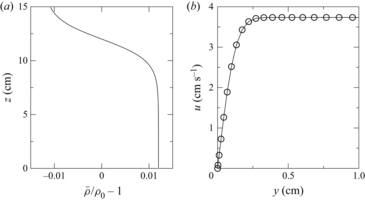
Figure 2. (a) The background stratification. (b) Along-channel velocity near the sidewall at the surface,  $z=15\ \textrm {cm}$, and the crest of the wave once the boundary layer has fully developed for a 2 cm amplitude wave.
Although the wavelength is partially constrained by the size of the domain, this constraint has minimal influence on the wave. We concern ourselves with waves of amplitude and wavelength which adequately fit within this DJL computational domain. Comparison between waves of amplitude 2 cm formed in a 1 m and 4 m long domain showed that the wave amplitude, speed and wavelength changed by 2 %,  $1\,\%$ and 6 %, respectively. Since the wave was only marginally affected by the choice of domain, we have used the shorter length to minimize computational costs.
We define the Reynolds number as  $Re = c L_w /\nu$. Except for § 3.2.5 which looks at the Reynolds number dependence of the interaction of the wave and constriction, we have used a consistent value of viscosity,
 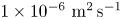 $1\times 10^{-6}\ \textrm {m}^2\,\textrm {s}^{-1}$, for all simulations. Due to the dependence of wave speed and wavelength on the wave amplitude, the Reynolds number varied between
  $2.4\times 10^4$ and
  $3.1\times 10^4$.
For large amplitude ISWs, a global instability may arise in the adverse pressure gradient within the BBL when the bottom boundary condition is no slip (Bogucki & Redekopp Reference Bogucki and Redekopp1999; Stastna & Lamb Reference Stastna and Lamb2008; Aghsaee et al. Reference Aghsaee, Boegman, Diamessis and Lamb2012; Sakai, Diamessis & Jacobs Reference Sakai, Diamessis and Jacobs2020). Although our bottom condition is free slip, this instability could still form along the no-slip sidewalls. Carr, Davies & Shivaram (Reference Carr, Davies and Shivaram2008) and Diamessis & Redekopp (Reference Diamessis and Redekopp2006) demonstrated that the instability only formed above a critical wave amplitude dependent on the Reynolds number. For comparison to these authors who used the water depth and linear wave speed in the definition of the Reynolds number, we find the Reynolds number to be  $1.1\times 10^4$. Because the wave amplitudes used here are below the critical value for this Reynolds number, no global instability is expected nor is it observed in our numerical experiments.
With the intention of limiting the diffusion of the moderately sharp background stratification, the diffusivity was fixed at  $1\times 10^{-7}\ \textrm {m}^2\,\textrm {s}^{-1}$, giving a Schmidt number
  $Sc = \nu /\kappa = 10$.
Computations were completed with a resolution of  $N_x \times N_y \times N_z = 1024 \times 96 \times 128 \approx 1.3\times 10^7$ points. The along-tank and vertical grid cells were equispaced with widths
  $\Delta x \times \Delta z = 0.20\ \mathrm {cm} \times 0.12\ \mathrm {cm}$. Because the across-tank dimension used a Chebyshev grid, the grid cells varied in size with a maximum width of
 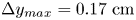 $\Delta y_{max} = 0.17\ \mathrm {cm}$. For a typical wave, the estimated boundary layer thickness,
  $\delta \sim L_w / \sqrt {Re} \approx 0.24\ \textrm {cm}$, agreed well with the thickness observed in the simulation (figure 2b). Because the Chebyshev grid clusters points near the boundary there are approximately ten grid points within this boundary layer, a suitable resolution for a pseudo-spectral DNS. Although there are no initial boundary layers in the solution of the DJL equation, boundary layers along the no-slip sidewalls form within a couple time steps and do not adjust the ISW significantly until the passage of the wave past the constriction.
Simulations were completed on Compute Canada's high performance system Graham using 16 processors. A typical simulation took approximately 4000 steps with an average time step of  $\Delta t \approx 6\ \textrm {ms}$. At this average rate, simulations routinely took a wall-clock time of 48 h for moderate wave amplitude. This is an excellent efficiency, especially for maintaining spectral accuracy with the resolution and the low number of processors.
We estimate the viscous dissipation rate as  $\epsilon =u_*^3/\ell$, where
  $u_*$ is the sidewall shear velocity and
  $\ell =3\ \textrm {cm}$ is the upper layer depth. From this, the Kolmogorov length scale can be estimated as
  $\eta _k = (\nu ^3/\epsilon )^{1/4} = (\nu ^3 \ell /u_*^3)^{1/4}$. A typical simulation has
  $u_*\sim 0.3\ \textrm {cm}\,\textrm {s}^{-1}$, giving a Kolmogorov length scale of 0.1 cm. This is well within an order of magnitude of the grid resolution, which has been proposed as sufficient resolution for a simulation to be called a DNS (Arthur & Fringer Reference Arthur and Fringer2014). Furthermore, the majority of the dissipation occurs within the boundary layer near the crest of the constriction where the lateral resolution is greatest.
Two passive tracers were included to measure lateral cross-side-boundary transport near the constriction, and vertical transport of pycnocline fluid. These tracers are called the wall tracer,  $T_w$, and pycnocline tracer,
  $T_p$, respectively. The diffusivity of the tracers was the same as that of the density field,
  $\kappa$. Their initial conditions are
 \begin{gather} T_w = \frac{1}{2} \left[ 1 + \tanh\left( \frac{y - (L_y - S(x) - d_w)}{h_w} \right) \right], \end{gather}
 \begin{gather}T_p = \frac{1}{2} \left[ \tanh\left( \frac{z-(z_0-d_p+\eta)}{h_p} \right) - \tanh\left( \frac{z-(z_0+d_p+\eta)}{h_p} \right) \right], \end{gather}
where  $\eta$ is the solution of the DJL equation. Parameters
  $d_w=1.5\ \textrm {cm}$ and
  $h_w=1.5\ \textrm {cm}$ define the thickness of the wall tracer and the transition length for
  $T_w$.
  $T_p$ has similar parameters setting the thickness,
  $d_p=1\ \textrm {cm}$, and transition thickness,
  $h_p=1.5\ \textrm {cm}$.
3. Results
3.1. Qualitative results
3.1.1. DJL cases
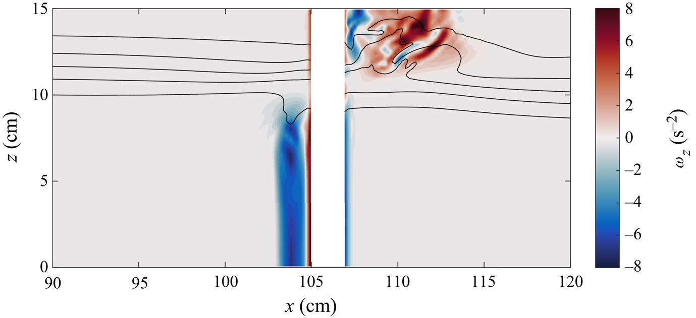
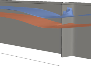
The typical behaviour of the interaction of an ISW with the sidewall constriction is shown in figure 3 for the base case. The base case consisted of an ISW with amplitude of 2 cm, and a constriction with amplitude of 3 cm and width of 2 cm. The wave travelled from the left to the right and induced a change in the isopycnals near the crest of the constriction. As the ISW began to pass the constriction, isopycnals within the wave were deflected vertically (figure 3a,b). In the upper portion of the pycnocline, the isopycnals were deflected upwards in a corkscrew shape on the upstream side of the constriction (in a reference frame moving with the wave). This is reversed in the lower portion of the pycnocline which was deflected downwards on the downstream side of the constriction. As the wave passed the constriction and the wave-induced velocities increased near the crest of the wave, the corkscrews broadened in width and height with the upper corkscrew nearly reaching the surface of the tank (figure 3c). As the wave left the constriction behind, the vertical isopycnal deflection began to return to equilibrium depth (figure 3d), although this isopycnal deflection persisted until the wave was well past the constriction. Although the constriction was on one side of the channel, the wave front remained perpendicular to the along-channel axis and did not rotate due to possible enhanced drag at the constriction.

Figure 3. Snapshots of the 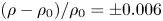 $(\rho -\rho _0)/\rho _0={\pm }0.006$ isopycnals as viewed from an angle for the base case with
  $a=2\ \textrm {cm}$,
  $A=3\ \textrm {cm}$ and
  $\sigma =2\ \textrm {cm}$ as the wave travels from left to right. As the wave passed the constriction, the upper portion of the pycnocline was drawn up into a large vortex on the upstream side of the constriction. To a smaller extent, the lower portion of the pycnocline was drawn down into a weaker vortex on the downstream side of the constriction. Movie available online.
  $(a)\ t = 6\ {\rm s},\, (b)\ t = 8\ {\rm s},\, (c)\ t = 10\ {\rm s},\, (d)\ t = 12\ {\rm s}.$
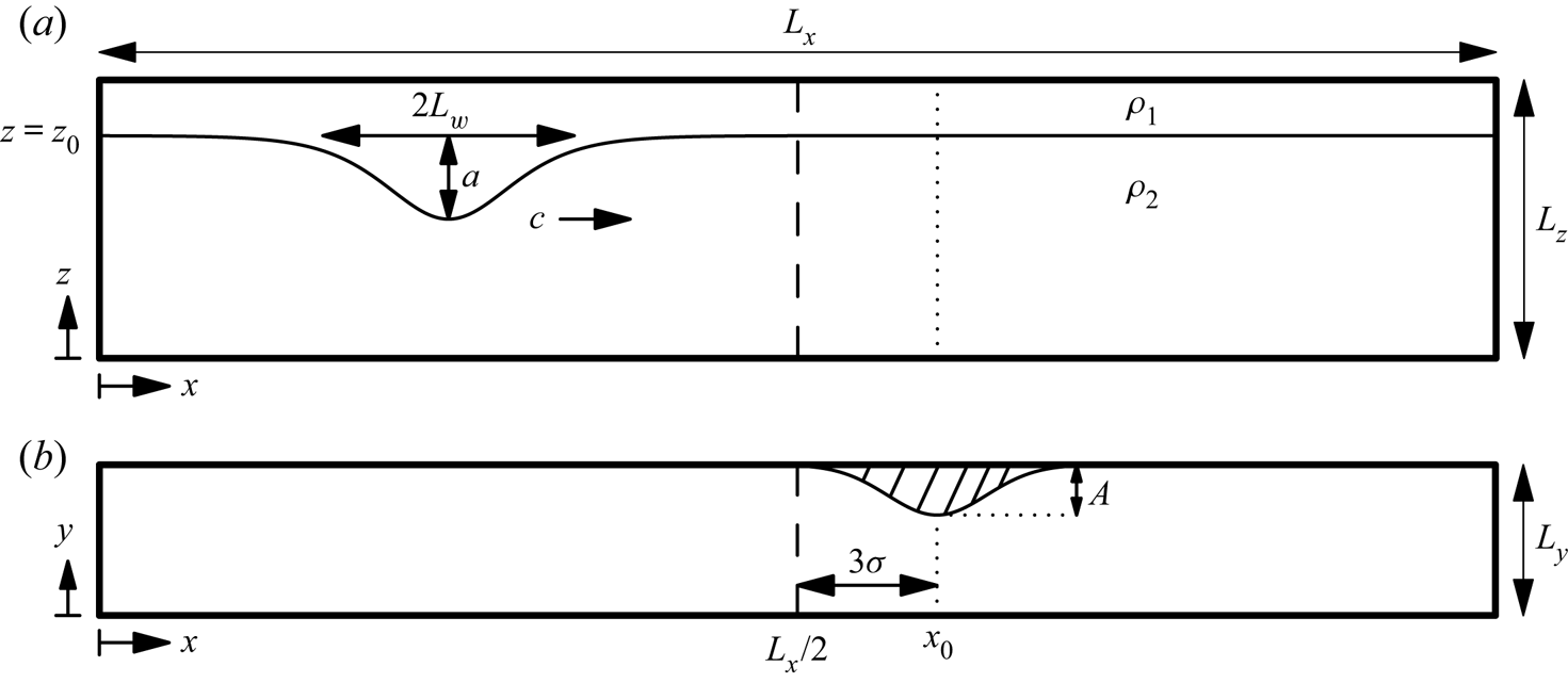
The corkscrew pattern is indicative of strong vertical vorticity, as confirmed by the cross-section in figure 4. Two vortices were generated when the wave passed the constriction; a strong vortex in the upper layer and a moderate strength vortex in the lower layer. Because the upper vortex is strong, constrained in a shallower layer and induced greater vertical isopycnal transport, it did not remain as coherent as the lower layer vortex. Based on the conservation of mass, the along-channel velocities associated with the ISW are larger in the upper layer than the lower because of the relative depths of each layer. Consequently, the magnitude of the vortices is also proportional to these layer velocities. For the base case shown in figure 3, the ratio of maximum absolute wave-induced velocities between the layers is approximately 2 whereas the ratio of the maximum absolute vertical vorticity (neglecting the boundary layer) is approximately 1.5.

Figure 4. Cross-section of vertical vorticity,  $\omega _z$, at
  $y=7.5\ \textrm {cm}$ after the wave has passed the constriction for the case shown in figure 3. Black density contours are overlaid with values
  $(\rho -\rho _0)/\rho _0=0,{\pm }0.004,{\pm }0.008$. The upper vortex is larger in width and is associated with the elevation of isopycnals. The lower vortex is weaker and does not draw down isopycnals as far as the upper vortex.
The vortex locations differed by layer. As a result of the opposing horizontal wave induced velocities in each layer, the upper layer vortex was upstream of the constriction, whereas the vortex was downstream in the lower layer. Since flow separation occurred near the crest of the hill, the vorticity was advected in opposite directions in each layer. For the same reasons, the orientation of the vertical vorticity was different in each layer.
A full description of the resultant flow features from the wave–constriction interaction are evident in the space–time plot of figure 5. The incident wave, initialized from the solution of the DJL equation, travelled at a constant speed towards the constriction. Upon reaching the constriction, the narrow channel width caused the wave-induced velocities to temporarily increase in magnitude before the wave continued its propagation down the channel. In general, the wave speed and wavelength remained constant throughout a simulation, while the wave amplitude decreased by up to 10 %.
Figure 5. Space–time plot of the along-channel velocity along the centre of the channel at the surface (i.e.  $z=15\ \textrm {cm}$ and
  $y=2\ \textrm {cm}$).
Two distinct responses are generated at the constriction. The first is the boundary-induced vorticity already discussed, while the second is small amplitude reflected waves. These waves typically have amplitudes that are 5 %–10 % of the incident ISW amplitude, although this ultimately depends on the properties of the constriction. Because the energy within these waves is often small compared to the vortices, we will not discuss them again until the discussion on energy in § 3.2.4. We will note that, on larger scales, secondary internal waves were observed in simulations of an internal surge in Cayuga Lake (a 60 km long, 5 km wide, channel-like lake) after interaction with sidewall features (Dorostkar et al. Reference Dorostkar, Boegman and Pollard2017).
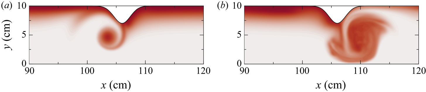
The vortices formed by the passage of the ISW significantly affected the two passive tracers,  $T_w$ and
  $T_p$, even for cases of low wave amplitude. Although not shown, the pycnocline tracer was advected vertically in a similar form to that seen in the density contours in figure 4. The wall tracer after the wave passed the constriction shows that the vortices scoured material from the sidewall into the interior of the channel (figure 6). It is clear that the amount and areal extent of the wall tracer scoured in the lower layer was less than that in the upper layer. The temporal evolution of
  $T_w$ reveals that the lower layer vortex remained coherent for the duration of the simulation, while the upper layer vortex had more variability (as also seen in figure 4).

Figure 6. Wall tracer,  $T_w$, for the case shown in figure 3 after the wave has passed the constriction (
 $t=20\ \textrm {s}$) in (a) the lower layer at
  $z=1\ \textrm {cm}$ and (b) the upper layer at
  $z=14\ \textrm {cm}$.
3.1.2. Forced flow
The complicated dynamics between the vortex, the ISW and the shear associated with the ISW can be simplified by removing the ISW and forcing the shear layer by a body force. Secondary simulations were completed, where the background stratification was advected by an added body force and no solitary wave field was prescribed. To approximate the vertical shear associated with the passage of an ISW, the body force was chosen to create a shear flow centred on the pycnocline. In this case, the  $u$-momentum equation of the Navier–Stokes equations, (2.3a), has the additional term
 \begin{align} F(z,t) = \frac{M_f}{\sqrt{\rm \pi}\varDelta} \exp\left[ -\left( \dfrac{t-t_c}{\varDelta} \right)^2 \right] \left\{ \tanh\left( \frac{z-z_0}{h} \right) + \frac{h}{L_z}\ln\left( \frac{\cosh{\dfrac{-z_0}{h}}}{\cosh\dfrac{L_z-z_0}{h}} \right) \right\}, \end{align}
where  $M_f$ determines the strength of the forcing,
  $t_c$ is the time of maximum forcing and
  $\varDelta$ is the transition time of the forcing. The right-most term in the curly brackets is included to remove the mean flow. For comparison, a purely barotropic current is initialized with a forcing of
 \begin{equation} F(z,t) = \frac{M_f}{\sqrt{\rm \pi}\varDelta} \exp\left[ -\left( \frac{t-t_c}{\varDelta} \right)^2 \right]. \end{equation}
 When no lateral boundaries are present, the resultant shear flow can be calculated from the time integral of (3.1). When the forcing has been switched off ( $t\gg t_c$) the resultant shear flow is
 \begin{equation} u(z) = M_f \left\{ \tanh\left( \frac{z-z_0}{h} \right) + \frac{h}{L_z}\ln\left( \frac{\cosh{\dfrac{-z_0}{h}}}{\cosh\dfrac{L_z-z_0}{h}} \right) \right\}. \end{equation}
Although this set-up is suitable for the study of shear instabilities such as Kelvin–Helmholtz or Holmboe instabilities, these instabilities are not of interest to the present work and we will ensure that their generation is limited. These instabilities form when the ratio of stratification to background shear is low, as characterized by the gradient Richardson number,
 \begin{equation} Ri = \frac{N^2}{u_z^2}. \end{equation}
Using (2.2) and (3.3), the minimum Richardson number is calculated to be
 \begin{equation} Ri_{min} = \frac{g h \Delta\rho}{2 M_f^2 \rho_0}. \end{equation}
Using representative values which form a similar shear flow to that of the ISW in figure 3 gives  $Ri_{min} = 10.9$. Because this value is well above the necessary condition, shear instabilities are not expected within these forced flow simulations or those with an ISW, nor were they observed.
The domain for this simulation was ( $L_x,L_y,L_z$) = (50 cm, 15 cm, 10 cm), and had the constriction located at
  $x_0 = 25\ \textrm {cm}$. Similar resolution to the DJL suite of simulations was used (
 $N_x \times N_y \times N_z = 512 \times 96 \times 128\approx 6.3\times 10^6$).
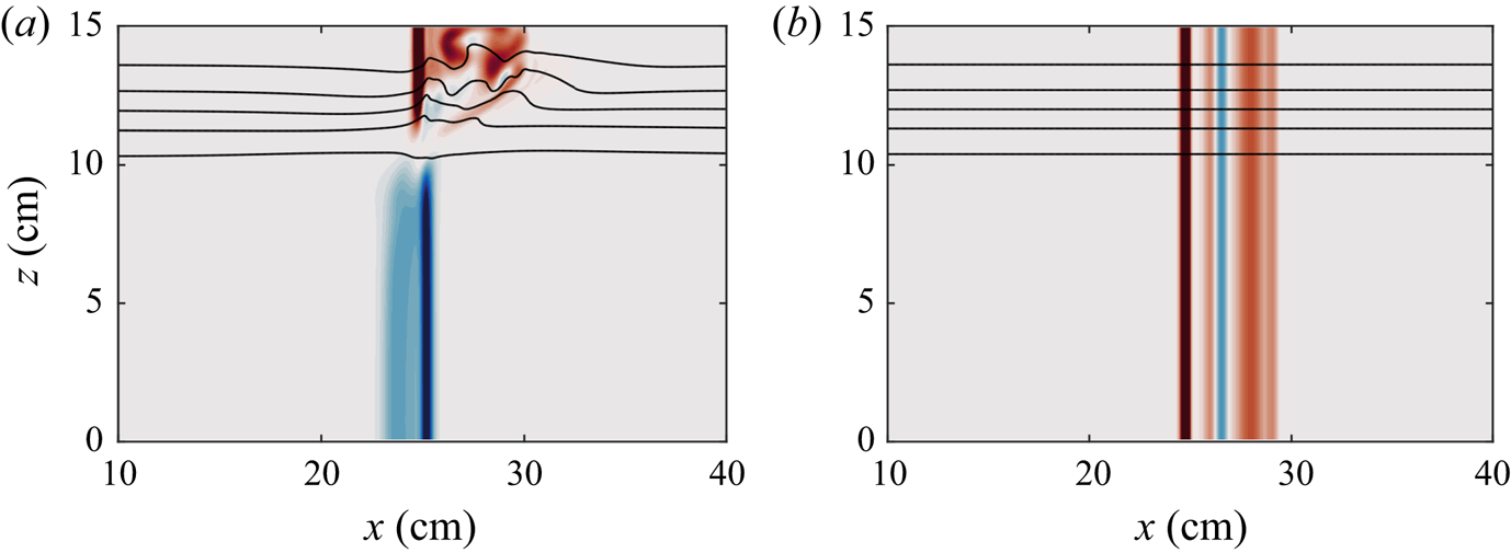
Figure 7(a) shows the vertical vorticity after the shear layer has developed for a background stratification equivalent to the ISW case just presented. Having matched the maximum horizontal velocity and thus the shear, the isopycnal deflection and the vorticity structure are comparable to that of figure 4. Most telling is the tilt in the vortex structure within the pycnocline.


We emphasize the importance of the shear as the source of the isopycnal deflection. The shear caused each vortex to rapidly change direction and magnitude at the interface. This vertical gradient in vorticity and velocity must be balanced with a lateral pressure gradient which is maintained by lateral density gradients. The inherent presence of shear within an ISWs necessitates this vertical transition, regardless of the form of stratification or sidewall constriction. That said, a stratification with a higher vertical density gradient will exhibit waves with greater shear along that gradient which will then induce a greater vertical gradient in the vorticity. This will in turn induce greater vertical isopycnal deformation.
Comparing this shear flow to a uniform-in-depth flow (figure 4b) shows that the barotropic current passing a constriction creates a depth-invariant vortex which leaves the pycnocline completely unaffected. Although there was no vertical deflection of the density or pycnocline tracer, the vortices formed by the barotropic current still scoured material from the sidewall into the interior, as in the shear case.
This barotropic flow is what is commonly observed as a tidal current past a headland (Signell & Geyer Reference Signell and Geyer1991; Canals et al. Reference Canals, Pawlak and MacCready2009). Comparison of these results is made to the study by Canals et al. (Reference Canals, Pawlak and MacCready2009), which demonstrated that a tilted vortex caused isopycnals to rise and fall due to vertical shear in azimuthal velocity around the vortex core. To be clear, their shear was significantly weaker than the rapid transition seen in figure 7 because the vortex was tilted only  $5^\circ$ compared to
  $23^\circ$ for the upper vortex. A key distinction between our results and the authors’ findings are that we find that isopycnals are only deflected in one direction for each layer's vortex as opposed to the predicted rising and lowering within each vortex. It is the very rapid change in the vertical vorticity at the interface due to the tilting of vortex lines towards the constriction which induces a vertical pressure gradient which drives the isopycnal motion.
3.2. Quantitative results
Here, we quantify and relate the characteristics of each vortex, such as their magnitude and motions, to the isopycnal deflection, resultant density overturning and tracer transport as they depend on wave amplitude, constriction width and constriction amplitude.
3.2.1. Vertical isopycnal deflection
The most striking feature of the previous section is the vertical transport of the interface by the vertical gradient in vorticity. From figure 4, the interface is seen to approach the upper surface due to the upper layer vortex.
The magnitude of the isopycnal deflection due to the vortex within the upper layer is defined as the maximum elevation of the  $\rho =\rho _0$ isopycnal from the spanwise median of that same isopycnal,
 \begin{equation} h_u = \max\left\{ M_{BL} \left( \eta - \tilde{\eta} \right) \right\}, \end{equation}
where  $\eta$ is the depth of the
  $\rho =\rho _0$ isopycnal,
  $\tilde {\eta }$ is the spanwise median of
  $\eta$ and
  $M_{BL}$ is a mask to remove the boundary layer along the sidewalls. The mask removed the volume within 1 cm of the flat sidewalls, but did not follow the constriction because this is where the vorticity which deforms the isopycnals originates. The spanwise median of
  $\eta$ measured the deformation of the density due to the wave and was independent of effects due to the constriction and the boundary layers. The amplitude of the lower layer isopycnal deflection is calculated similarly as the maximum descent of the
  $\rho =\rho _0$ isopycnal from the spanwise median,
 \begin{equation} h_l = \max\left\{ M_{BL} \left( \tilde{\eta} - \eta \right) \right\}. \end{equation}
 The temporal evolution of the isopycnal deflections due to the upper and lower vortices is shown in figure 8. The left column shows the deflection for different wave amplitudes when the constriction shape remains constant. In the upper layer, the waves with larger amplitude induced greater isopycnal displacements relative to their incident amplitude. However, even the small 0.5 cm amplitude wave-induced vertical transport that was nearly 50 % of the initial wave amplitude. Although the maximum vertical isopycnal displacement within the upper layer is  $a+h_1$, where
  $h_1$ is the depth of the upper layer, we observe a maximum closer to
  $a$. Within the upper layer, the maximum isopycnal deflection occurred when the wave was centred on the constriction, but occurred 2–3 s later in the lower layer due to the weaker vorticity. The weaker velocities in the lower layer caused the maximum isopycnal descent within the lower layer to be approximately three times less than the maximum elevation in the upper layer.
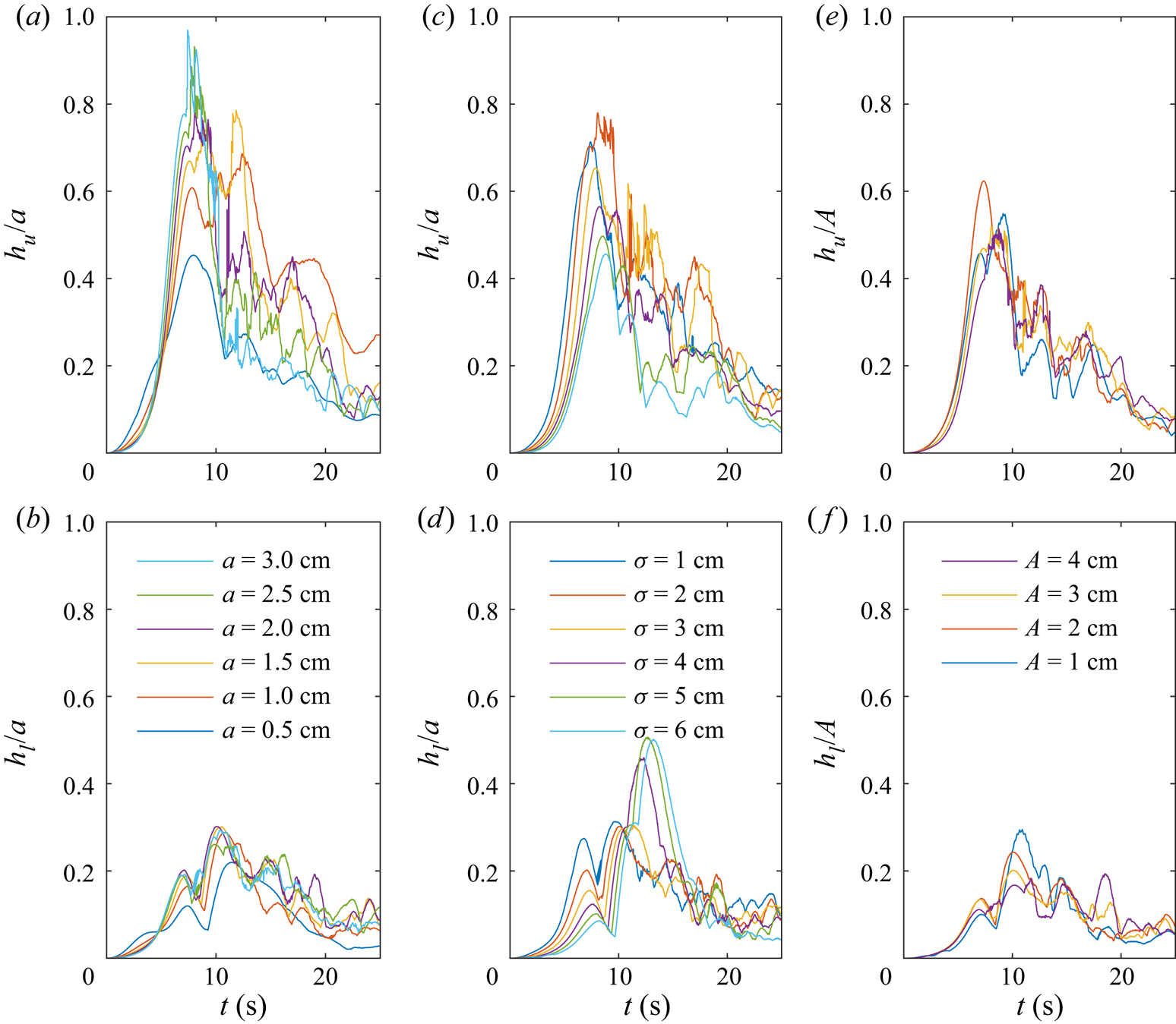
Figure 8. Height of the isopycnal deflection as a function of time in the (a,c,e) upper layer and (b,d,f) lower layer for (a,b) various wave amplitudes with  $A=3\ \textrm {cm}$ and
  $\sigma =2\ \textrm {cm}$, (c,d) various constriction widths with
  $a=2\ \textrm {cm}$ and
  $A=3\ \textrm {cm}$ and (e,f) various constriction amplitudes with
  $a=2\ \textrm {cm}$ and
  $\sigma =2\ \textrm {cm}$. Note that (e,f) are scaled by constriction amplitude,
  $A$, rather than wave amplitude,
  $a$.
$a$.
An increase in the width of the constriction caused a reduction in the upper layer deflection, but an increase in the lower layer (figure 8c,d). The first is expected since an increase in the constriction width would cause a decrease in the strength of the flow separation which is responsible for the vortex formation, as well as the isopycnal displacement. The latter is a boundary layer effect along the crest of the constriction. Since the boundary layer mask leaves the crest within the measurement domain, the wider constriction cases behave more like a flat wall. As the wave passed, the upper layer fluid that was brought down with the wave remained attached near the sidewall crest when the isopycnals returned to their equilibrium depth in the aft of the wave. The increase in the lower layer isopycnal deflection is a boundary layer effect rather than a result of the vertical vorticity.
Figure 8(e,f) demonstrates that the isopycnal deflection in the upper layer is proportional to the constriction amplitude when all else is held fixed. Combined with the observations for constrictions of different widths, the isopycnal deflection is greatest for narrow and large amplitude constrictions for which the strongest vorticity forms.
We have argued that the vortices are directly responsible for the vertical isopycnal deflection because of the rapid vertical gradient in velocity. This argument has been previously applied in the context of stratified vortices by Beckers et al. (Reference Beckers, Verzicco, Clercx and Van Heijst2001) and Canals et al. (Reference Canals, Pawlak and MacCready2009) who observed vertical isopycnal motion in the context of pancake-like vortices and tilted vortices, respectively. An expression demonstrating the connection between vorticity and the vertical isopycnal displacement arises in the idealized flow around a vortex core. Using cylindrical coordinates, assuming azimuthal symmetry, zero radial velocity, the steady Euler equations under the Boussinesq approximation in a non-rotating reference frame are
 \begin{gather} \frac{u_\theta^2}{r} = \frac{1}{\rho_0}\frac{\partial p'}{\partial r}, \end{gather}
 \begin{gather}\frac{\partial p'}{\partial z} ={-}\rho' g, \end{gather}
 \begin{gather}\frac{u_\theta}{r}\frac{\partial \rho'}{\partial \theta} ={-}\frac{\partial \rho'}{\partial z} u_z, \end{gather}
where the prime denotes perturbations from the background state. That is, the density and pressure can be decomposed such that  $\rho = \rho _0 + \bar {\rho }(z) + \rho '$ and
  $p = p_0(z) + p'$. Respectively, (3.8) describe the cyclostrophic balance, hydrostatic balance and conservation of mass. Combining (3.8a) and (3.8b) gives
 \begin{equation} \frac{\partial \rho'}{\partial r} ={-}\frac{\rho_0}{g} \frac{\partial}{\partial z}\left( \frac{u_\theta^2}{r} \right), \end{equation}
which is comparable to the expression for the thermal wind in a rotating stratified flow. More applicably, it becomes clear that a vertical gradient in the azimuthal velocity (i.e. the vorticity) is balanced by a lateral gradient of the density. Although, the isopycnals have horizontal gradients within the wave, these gradients are formed by the balance of nonlinear steepening and dispersion. Thus, the vertical shear of the vorticity must induce a local vertical transport of the interface.
The strength of the vertical gradient will depend on both the magnitude of the vorticity and the thickness of the interface. Because the thickness has remained fixed for all simulations, the height of the isopycnal deflection will depend primarily on the magnitude of the vorticity. The strength of the vortex in the upper and lower layers are defined using the vertical component of enstrophy normalized by the layer volume,
 \begin{gather} \varOmega_{u} = \frac{1}{2 V_u} \int_{V_u} \left( \omega_z M_{BL} \right)^2 \,\textrm{d}V, \end{gather}
 \begin{gather}\varOmega_{l} = \frac{1}{2 V_l} \int_{V_l} \left( \omega_z M_{BL} \right)^2 \,\textrm{d}V, \end{gather}
where  $V_u$ and
  $V_l$ are the volumes above and below the
  $\rho = \rho _0$ isopycnal, respectively.
If we assume the vorticity within a layer is proportional to the ratio of the azimuthal velocity,  $u_\theta$, and the width of the vortex,
  $R$, then the strength of the vortex is
 \begin{equation} \varOmega_u \sim \frac{u_\theta^2}{R^2}. \end{equation}
If we further assume that the vertical and radial gradients in (3.9) are approximately constant over the depth of the stratification,  $h$, and the width of the vortex, then combining (3.11) and (3.9) reveals
 \begin{equation} \frac{\Delta \rho'}{R} ={-}\frac{\rho_0 u_\theta^2}{gRh} \sim{-}\frac{\rho_0 R \varOmega}{gh}. \end{equation}
The density difference can be approximated by the background stratification over a particular depth. In the upper layer this would be
 \begin{equation} \Delta \rho' ={-}\left| \frac{\partial\rho}{\partial z} \right| h_u, \end{equation}
which when used in (3.12) gives
 \begin{equation} h_u \sim \left| \frac{\partial\rho}{\partial z} \right|^{{-}1} \frac{\rho_0 R^2 \varOmega_u}{gh}. \end{equation}
Comparison between the maximum isopycnal deflection and the maximum of the vertical component of enstrophy within each layer is shown in figure 9. In both the upper and lower layers, the height of the isopycnal deflection is dependent on the vorticity. Differences between constrictions of different widths are evident, and we speculate that this is related to the radius of the vortex. Unfortunately, it was impossible to systematically measure this radius, both because it increased over time and because during the early stages of vortex development the vortices did not have circular cross-sections.
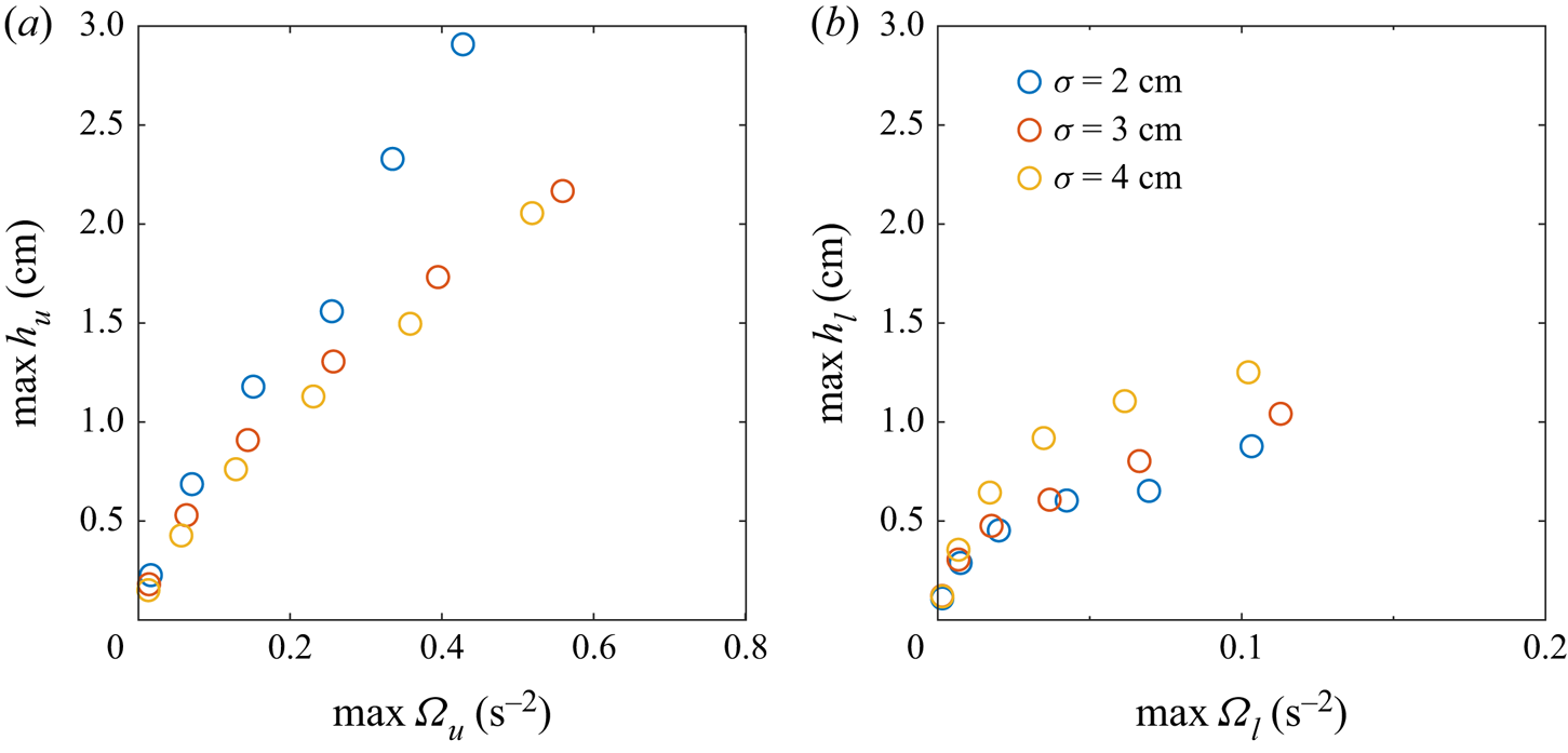
Figure 9. The dependence of the maximum isopycnal deflection on the maximum vertical component of enstrophy within the (a) upper and (b) lower layers. The constriction amplitude and width remained fixed at  $A=3\ \textrm {cm}$ and
  $\sigma =2\ \textrm {cm}$, respectively. Note the difference in the horizontal axes.
3.2.2. Vortex paths
The position of the vortices give indication as to the spatial range of the isopycnal deflection and an estimate of the spread of the wall tracer. Strong vertical motion was initially seen along the crest of the constriction, eventually moving into the interior of the channel as the vortex developed.
The position of the vortices was calculated from the centroid of the vertical vorticity within each layer. For the upper vortex, this is
 \begin{gather} x_u = \frac{1}{2 \varOmega_u V_u} \int_{V_u} x \left( \omega_z M_{BL} \right)^2 \,\textrm{d}V, \end{gather}
 \begin{gather}y_u = \frac{1}{2 \varOmega_u V_u} \int_{V_u} y \left( \omega_z M_{BL} \right)^2 \,\textrm{d}V, \end{gather}
Similar expressions for the centroid of the vortex in the lower layer,  $x_l$ and
  $y_l$, can be found using the volume below the
  $\rho =\rho _0$ isopycnal.
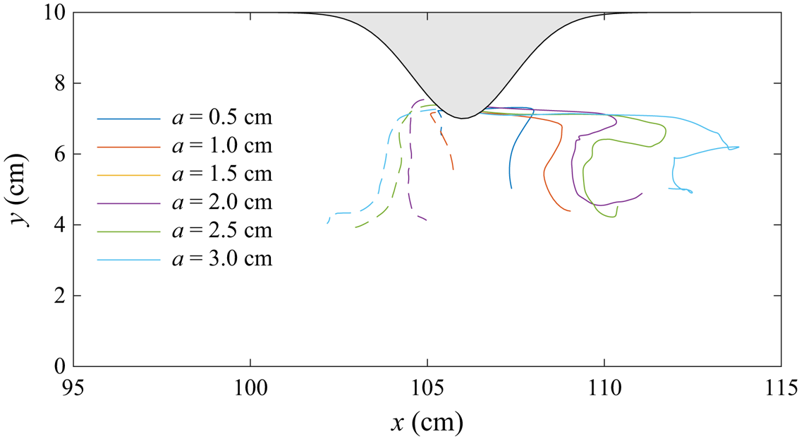
The vortex paths for a range of wave amplitudes with a fixed constriction is shown in figure 10. Tracks of the upper layer vortex (solid lines) and lower layer vortex (dashed lines) indicate that the vortices formed on either side of the constriction crest. The displacement of the upper layer vortex from the constriction increased with wave amplitude (and thus wave-induced velocities) due to the vortex being partially carried by the wave. Because this vortex was not fully caught within the wave, it left the rear of the wave and reversed its direction of travel from right to left. The vortex paths observed by Canals et al. (Reference Canals, Pawlak and MacCready2009) for tidal flow past a headland similarly showed directionality with the background tidal current. The lower layer vortex does not experience this Lagrangian drift because of the change in orientation of the wave-induced velocity. Although the cross-stream velocities from the wave are small, the vortices still travel to the mid-plane of the channel.

Figure 10. Tracks of the upper layer vortex (solid line) and the lower layer vortex (dashed line) for the cases shown in figure 8.
As seen in figure 6, the induced vortices scoured a portion of the sidewall tracer into the interior of the channel. The amount of tracer within the interior is quantified as,
 \begin{equation} T_{sc} = \int_V T_w M \,\textrm{d}V, \end{equation}
where  $M$ is a mask to remove the initial tracer near the constricting sidewall. This is an effective measurement of the lateral transport capabilities of the vortices.
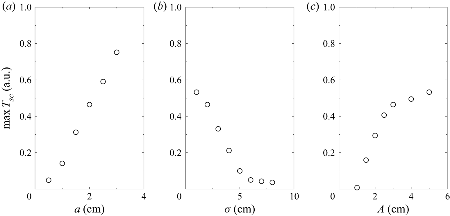
Figure 11 shows the maximum amount of wall tracer transported into the interior of the channel by the vortices. Larger wave amplitudes and narrow constrictions lead to significant tracer transport due to the strong vorticity. In contrast, limited tracer transport occurs for wide constrictions, where  $\sigma = 6\ \textrm {cm}$ is a critical value.

Figure 11. Maximum wall tracer,  $T_w$, scoured into the interior of the channel for (a) various wave amplitudes with
  $A=3\ \textrm {cm}$ and
  $\sigma =2\ \textrm {cm}$, (b) various constriction widths with
  $a=2\ \textrm {cm}$ and
  $A=3\ \textrm {cm}$ and (c) various constriction amplitudes with
  $a=2\ \textrm {cm}$ and
  $\sigma =2\ \textrm {cm}$.
The tracer transport increased with constriction amplitude and can be characterized by two critical values. First, is the minimum amplitude for significant vortex generation necessary to transport material away from the sidewall. This value is close to  $A=1\ \textrm {cm}$ for a 2 cm amplitude wave. As the vortices grew in magnitude with increasing constriction amplitude, they reached a magnitude where all neighbouring tracer was cleared into the interior of the channel. This second critical amplitude is approximately
  $A=3\ \textrm {cm}$.
It is well known that cross-boundary layer transport and resuspension of bottom material exists within the footprint of an ISW (Bogucki & Redekopp Reference Bogucki and Redekopp1999; Quaresma et al. Reference Quaresma, Vitorino, Oliveira and da Silva2007; Harnanan, Soontiens & Stastna Reference Harnanan, Soontiens and Stastna2015). Resuspension within the BBL, however, will remain trapped below the stratified region unless the wave shoals along a sloping boundary, thereby changing form and possibly creating nepheloid layers of resuspended material (Bourgault et al. Reference Bourgault, Morsilli, Richards, Neumeier and Kelley2014; Masunaga et al. Reference Masunaga, Arthur, Fringer and Yamazaki2017) or a bolus (Arthur & Fringer Reference Arthur and Fringer2016). However, within long fjords and lakes, the shoaling will primarily occur at the ends of the channel. Thus the vortex generation mechanism described herein is a means for tracer transport from the boundaries into the interior at any point along the lake with significant shoreline features (e.g. headlands). Such was the case in Upper Lake Constance where coherent vertical isopycnal displacements along with enhanced mixing and density overturning was observed in the near-shore region of an ISW travelling perpendicular to the shore (Preusse & Peeters Reference Preusse and Peeters2014).
3.2.3. Density overturning
The generated vorticity and its influence on the tracer and density fields is evident in cases of large wave amplitude, constriction amplitude, or narrow constriction width. Although the vortices locally raised and lowered the isopycnals, they often did so in a chaotic manner due to inherent instability caused by both the shear and the nearby boundary. This instability is able to cause the isopycnals to overturn, thereby inducing local mixing.
We define the overturning height as
 \begin{equation} h_{ot} = \max_{(x,y)}\left\{ z_1(x,y) - z_2(x,y) \right\}, \end{equation}
where  $z_1$ and
  $z_2$ are the maximum and minimum heights of the
  $\rho =\rho _0$ isopycnal at a horizontal position. Although this overturning length scale overestimates the Thorpe scale, it will suffice as a simple proxy for the mixing potential.
Figure 12 shows the maximum overturning height for the base case. Density overturning occurred rapidly when the wave reached the constriction and persisted until after the wave passed. Compared to the amplitude of the wave (2 cm), the maximum overturning height is comparable ( $h_{ot}=1.5\ \textrm {cm}$).
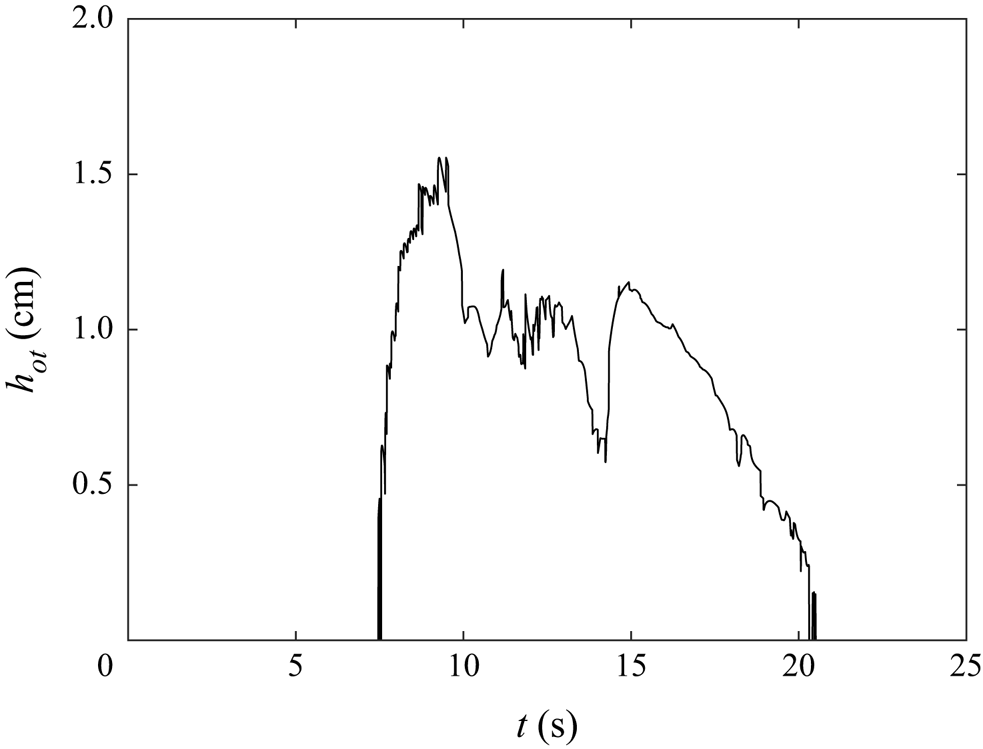
Figure 12. Overturning height for the base case ( $a=2\ \textrm {cm}$,
  $\sigma =2\ \textrm {cm}$ and
  $A=3\ \textrm {cm}$).
The maximum overturning height for various configurations is shown in figure 13. Overturning is found to increase with wave amplitude and constriction amplitude. It was anticipated that the density overturning would increase with decreasing constriction width because the vortices would be more energetic as the constriction approached a knife edge. However, the opposite was true. As the constriction width decreased the widths of the vortices increased which created a broader isopycnal deformation. This makes the overturning of density more difficult as it requires a greater lateral displacement to achieve an equivalent overturning height. Thus, there is an intermediate region where the constriction is narrow enough to induce significant vorticity, but wide enough to form thin vortices. No overturning was observed for constrictions wider than 6 cm. As this is considerably narrower than the wavelength of the wave ( $44\ \textrm {cm}$) the flow is expected to remain stable for most constrictions.
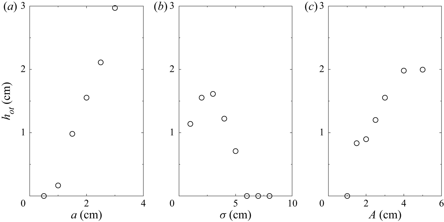
Figure 13. Maximum density overturning height for (a) various wave amplitudes with  $A=3\ \textrm {cm}$ and
  $\sigma =2\ \textrm {cm}$, (b) various constriction widths with
  $a=2\ \textrm {cm}$ and
  $A=3\ \textrm {cm}$ and (c) various constriction amplitudes with
  $a=2\ \textrm {cm}$ and
  $\sigma =2\ \textrm {cm}$.
The trends in overturning magnitude are comparable to those seen in figure 11 for the wall tracer carried by the vortices into the interior of the fluid. Because both of these features are a direct consequence of the induced vortices, it is unsurprising to see these similarities. The vertical mixing due to the overturning is therefore directly linked with the lateral spreading of sidewall material.
3.2.4. Energy extracted from incident ISW
The vortices are the primary response to the transit of the ISW past the constriction. Since the only source of available mechanical energy (sum of kinetic and available potential energy) is within the incident ISW, a transfer of energy from the wave into the vortices must occur.
Following the energy budget formulation of Winters et al. (Reference Winters, Lombard, Riley and D'Asaro1995), the total kinetic and potential energy within the fluid domain, denoted with volume  $V$, is
 \begin{gather} E_k = \frac{\rho_0}{2}\int_V (u^2 + v^2 + w^2) \,\textrm{d}V, \end{gather}
 \begin{gather}E_p = \int_V \rho g z \,\textrm{d}V. \end{gather}
In the absence of boundary fluxes, the components of the rate of change of kinetic and potential energy are
 \begin{gather} \frac{\textrm{d}^{} E_k}{\textrm{d} t^{}} ={-}\phi_z - \epsilon, \end{gather}
 \begin{gather}\frac{\textrm{d}^{} E_p}{\textrm{d} t^{}} = \phi_i + \phi_z, \end{gather}
where  $\phi _z$ is the reversible vertical buoyancy flux rate,
  $\epsilon$ is the viscous dissipation rate and
  $\phi _i$ is the irreversible rate of conversion from internal energy to potential energy through diffusion. These are defined as
 \begin{gather} \phi_z = \int_V \rho g w \,\textrm{d}V, \end{gather}
 \begin{gather}\epsilon = \int_V 2\mu e_{ij} e_{ij}\,\textrm{d}V, \end{gather}
 \begin{gather}\phi_i = g \kappa \int_{A} \rho(z=0) - \rho(z=L_z) \,\textrm{d}A, \end{gather}
where  $e_{ij} = ({\textrm {d}u_i}/{\textrm {d}x_j} + {\textrm {d}u_j}/{\textrm {d}x_i})/2$ is the strain rate tensor.
The potential energy may be partitioned into the available potential energy,  $E_{a}$, and the background potential energy,
  $E_{b} = \int _V \rho (z_*) g z_* \,\textrm {d}V$, where
  $E_p = E_a + E_b$. Conceptually, the background potential energy is the minimum potential energy of the system through an adiabatic redistribution of density, where
  $z_*$ denotes the vertical position of the sorted density field over the entire fluid domain;
  $E_a$ is then realized as the energy available to be converted into kinetic energy.
Using this partition of potential energy, the total available mechanical energy is
 \begin{equation} E_{TA} = E_k + E_a = E_k + E_p - E_b, \end{equation}
with a rate of change of
 \begin{equation} \frac{\textrm{d}^{} E_{TA}}{\textrm{d} t^{}} ={-}(\phi_d - \phi_i) - \epsilon, \end{equation}
where  $\phi _d = {\textrm {d}E_b}/{\textrm {d}t}$ includes increases in the background potential energy due to irreversible mixing.
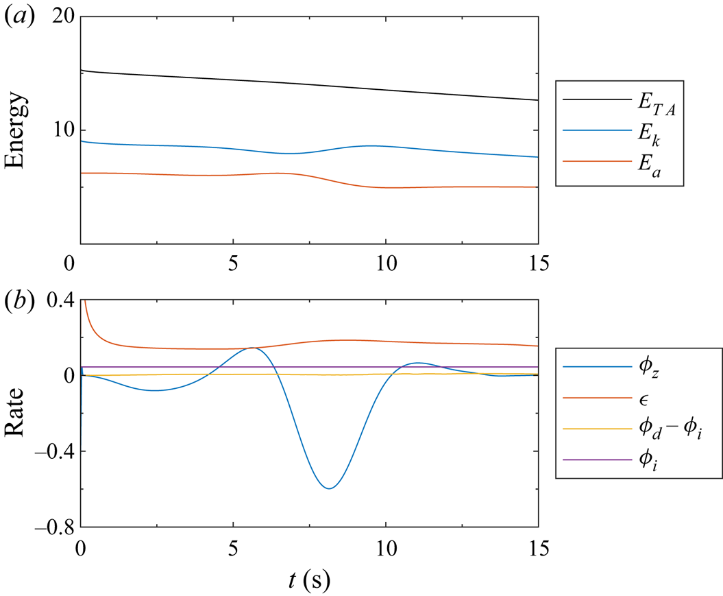
The energy components and instantaneous rates of change for the base case give an indication as to the source of the energy within the vortices. Figure 14(a) shows that the total available energy decreases consistently due to viscous dissipation and, to a negligible extent, through mixing and diffusion of the interface (figure 14(b) compares the instantaneous rates). However, these do not influence the formation of the vortices or the reflected waves, which can be seen in the conversion between the kinetic and potential energies. The potential energy remained relatively constant until the wave reached the constriction around  $t=6\ \textrm {s}$, at which time potential energy began to convert into kinetic energy in the form of the vortices and reflected waves. There will be some increase in the potential energy due to the isopycnal deflection, but this contribution will be overwhelmed by the kinetic energy within the vortices. After the wave passed the constriction, the potential energy remained constant again, albeit 20 % lower in value. The loss of potential energy is in agreement with the decrease of 10 % in the wave amplitude when comparing the wave before and after the constriction.

Figure 14. (a) Time evolution of total available, kinetic and available potential energies. (b) Instantaneous rates of energy transfer. The units are arbitrary.
The amount of potential energy within the wave that is converted into the kinetic energy of the vortices and the reflected waves will depend on a number of factors, the most significant are the incident wave amplitude, and the amplitude and width of the constriction. The percentage of kinetic energy within the vortex and reflected waves relative to the kinetic energy in the transmitted wave is shown in figure 15. The kinetic energy within the reflected waves is less than that within the vortex except when the constriction width is large, in which case only weak vortices formed. The kinetic energy within the vortices and the reflected waves show little dependence on the incident wave amplitude. This indicates that the flow separation causing the vortices increased in tandem with the kinetic energy within the wave. Unsurprisingly the constriction amplitude had the greatest influence on the kinetic energy within the vortices and the reflected waves. As the constriction amplitude approached half the domain width ( $A=5\ \textrm {cm}$) the waves and vortex accounted for 23 % of the residual kinetic energy. However, this is a sizeable constriction amplitude relative to the channel width with little likelihood of being realized in geophysical flows.

Figure 15. Ratio of kinetic energy within the vortices to the kinetic energy within the wave for (a) various wave amplitudes with  $A=3\ \textrm {cm}$ and
  $\sigma =2\ \textrm {cm}$, (b) various constriction widths with
  $a=2\ \textrm {cm}$ and
  $A=3\ \textrm {cm}$ and (c) various constriction amplitudes with
  $a=2\ \textrm {cm}$ and
  $\sigma =2\ \textrm {cm}$.
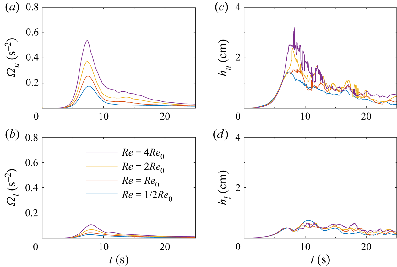
3.2.5. Reynolds number dependence
In the field, the relative size of the viscous boundary layer to the constriction amplitude is small. To extrapolate the results of the above laboratory scale to situations with larger length scales, we adjusted the boundary layer thickness through its dependence on the Reynolds number ( $\delta \propto Re^{-1/2}$). Four cases are compared by varying the viscosity by factors of two. To ensure proper resolution of the boundary layer the number of grid cells in the spanwise (Chebyshev) direction was increased from 96 to 160 in the largest Reynolds number case. Using the scaling for the law of the wall,
  $y^+ = y u_\tau / \nu$ where
  $u_\tau = \sqrt {\nu (\partial {u}/\partial {y})|_{y=0}}$, the tenth grid point decreased from 7 to 6 wall units from the wall. Although the Kolmogorov length scale decreased by a factor of 3 in this case, the resolution remained within the classification of a DNS. Inspection of the energy budget showed no significant energy extraction by non-physical elements of the numerical model.
With increasing Reynolds number, the flow separation is easier to induce due to less viscous traction along the boundary. This then leads to the formation of stronger vortices at higher  $Re$ (figure 16a,b). Comparison between the vortices in all cases shows them to be approximately the same size. As a result, the isopycnal displacement also increases with Reynolds number due to (3.14).

Figure 16. Vertical component of enstrophy (a,b) and the height of isopycnal deflection (c,d) in the upper layer (a,c) and lower layer (b,d). The base Reynolds number was  $Re_0 = 2.4\times 10^4$.
Extending to field scales, the Reynolds number based on the molecular diffusivity is orders of magnitude larger than those within a laboratory due to the larger length and velocity scales. However, the eddy diffusivity is likely more suitable at these larger scales. In the open ocean, the eddy diffusivity of ISWs is of the order of  $10^{-5}\ \textrm {m}^2\,\textrm {s}^{-1}$ but can be in the range
  $10^{-2}\text {--}10^{-1}\ \textrm {m}^{2}\,\textrm {s}^{-1}$ when shoaling (Bogucki, Dickey & Redekopp Reference Bogucki, Dickey and Redekopp1997; Van Haren & Gostiaux Reference Van Haren and Gostiaux2012). In the case of Bogucki et al. (Reference Bogucki, Dickey and Redekopp1997) the Reynolds number using the eddy diffusivity is approximately 600, significantly smaller than the values used above.
4. Discussion and conclusions
In this work we demonstrated that vortices were generated above and below the pycnocline when an ISW passed a narrow (relative to the wavelength) sidewall constriction. Each vortex provided a means of coherent transport of material away from the near-sidewall region as well as vertical displacement of the interface due to a pressure drop in the interior of the vortices. In the upper layer, the vortex was found to raise pycnocline fluid near to the surface for large amplitude, narrow constrictions or large amplitude waves. Below the deformed pycnocline the vortex was weaker and remained coherent far longer, although both the coherent transport of material away from the near-sidewall region and the vertical isopycnal displacement were consistent with what was observed above the pycnocline.
The formation of the vertical isopycnal displacement was a consequence of the shear within the along-channel velocity component and thus the vertical vorticity. The height of the isopycnal displacement was proportional to the strength of the vertical vorticity. Although we have investigated vorticity, shear and isopycnal displacement due to ISWs, other mechanisms such as wake vortices (Bonnier, Eiff & Bonneton Reference Bonnier, Eiff and Bonneton2000), vortices due to mixing (Lelong & Sundermeyer Reference Lelong and Sundermeyer2005) and tidal flow through straits (Imasato et al. Reference Imasato, Fujio, Zhang, Awaji and Akitomo1994) may independently contribute to their formation.
Most laboratory and numerical studies of ISWs assume homogeneity of the wave along the wave crest. This is a valid assumption for waves within the open ocean where, although the wave fronts are often curved, the radius of curvature is large compared to the amplitude and wavelength of the wave. While the ISWs considered here initially agree with this assumption, the geometry of the boundaries created localized vorticity which broke this symmetry. Observations within Lake Constance showed that an ISW had substantial lateral variability as a result of increased mixing along the shore (Preusse & Peeters Reference Preusse and Peeters2014).
With this in mind, it is important to note the inherent three-dimensionality of the present situation. In contrast to many internal wave studies on breaking or BBL processes induced by such waves, the present situation does not begin as a two-dimensional primary instability (e.g. billows in the case of shear instability (Xu et al. Reference Xu, Stastna and Deepwell2019), or a separation bubble beneath shoaling internal waves Boegman & Stastna Reference Boegman and Stastna2019). In contrast to these instabilities, which typically have their vorticity oriented in a plane with constant density, the vorticity here is primarily directed normal to isopycnals. Instead of a localized instability, the wave interacts with the constriction across the entire water column over which the horizontal velocity varies. In this respect, the shear along the pycnocline acts to de-couple the two vortices which then evolve nearly independently of each other.
Comparison of the present situation can be made to that of Harnanan et al. (Reference Harnanan, Soontiens and Stastna2015) and Harnanan et al. (Reference Harnanan, Stastna and Soontiens2017), who considered near-bed instabilities caused by the passage of an ISW over a bump of similar form to our sidewall constriction. They observed two different instabilities which led to localized cross-boundary layer transport. The first of these instabilities was a roll-up of the trailing prograde jet formed by the adverse pressure gradient on the no-slip boundary, while the second is the more typical flow separation for topography with large slope. We have not observed the first instability, although it could be initiated at higher Reynolds number when the boundary layer thickness is thinner, or for a conjugate flow limited (i.e. flat-crested) wave. The localized material transport due to the flow separation is more comparable to our observations, however, the horizontal transport of near-wall material is substantial (see figure 6b) compared to the vertical transport of a few boundary layer widths in Harnanan et al. (Reference Harnanan, Soontiens and Stastna2015). Harnanan et al. (Reference Harnanan, Stastna and Soontiens2017) found that a near-bed stratification increased the three-dimensionalization and cross-boundary layer transport compared to a situation without near-boundary stratification. A sidewall, however, necessarily intersects the pycnocline, or in other words the dominant region of stratification. Thus, any instability formed by the wave will have a portion of which that exists within a stratified region. This region of stratified instability is then likely to have elevated three-dimensionality which was observed in the levels of density overturning.
Unlike typical vortex generation due to ISWs discussed in the literature for which the vorticity vector is aligned with isopycnals, such as shear instabilities in the main water column or global instabilities within the BBL, the vorticity generated here was necessarily perpendicular to the stratification. This produced energetic vortex tubes over a large vertical extent, and these coherent structures acted to transport passive and active scalars. Moreover, the coherent vortices evolved in fundamentally different ways to shear or BBL instability, which are far more localized in depth.
Significant literature exists on the instabilities of stratified vortices due to tilting (Boulanger, Meunier & Le Dizés Reference Boulanger, Meunier and Le Dizés2007; Boulanger, Meunier & Le Dizès Reference Boulanger, Meunier and Le Dizès2008), background shear (Basak & Sarkar Reference Basak and Sarkar2006; Billant & Bonnici Reference Billant and Bonnici2020) or of vortex pairs (Billant & Chomaz Reference Billant and Chomaz2000a,Reference Billant and Chomazb). Each of these instabilities could lead to a change in the dynamics of the vortices we have simulated. More physically relevant sidewalls with tilted boundaries would likely lead to enhanced vertical motion due to the enhanced shear caused by the tilt (similar to that of Canals et al. Reference Canals, Pawlak and MacCready2009). Depending on the strength, orientation and location of a background shear, vortices caused by ISWs could either be enhanced or diminished. Because ISWs often exist as members of a train of rank ordered ISWs, leading ISWs would create vortices which could interact with trailing ISWs and their induced vortices in ways possibly similar to Billant & Chomaz (Reference Billant and Chomaz2000a). Throughout this work it has been assumed that the background stratification has remained consistent, however, a thicker pycnocline or a stratified lower layer would create conditions with closer links to the above literature (which was largely concerned with linearly stratified fluids).
The choice of vertical sidewalls led to strong and clear vortex generation. However, headlands exist with sloping boundaries which add an additional source of vertical shear. Future studies on how the slope of the boundary influences ISWs and tidal currents will be more relevant to field scales, but will be substantially more complicated dynamically and numerically.
Supplementary movie
Supplementary movie is available at https://doi.org/10.1017/jfm.2021.25.
Acknowledgements
This project began while D.D. and C.C. were graduate and undergraduate students, respectively, at the University of Waterloo.
Funding
D.D. was funded by a QEII scholarship while at the University of Waterloo, and through an NSERC Discovery grant to Bruce Sutherland while a postdoctoral fellow at the University of Alberta. M.S. was funded by an NSERC Discovery grant RGPIN-311844-37157.
Declaration of interests
The authors report no conflict of interest.