


INTRODUCTION
Tropical rain forests greatly impact global climate by regulating exchange of greenhouse gases (GHGs) between terrestrial ecosystems and the atmosphere such as carbon dioxide (CO2), methane (CH4) and nitrous oxide (N2O), however, whether tropical rain forests function as a sink or a source for these GHGs needs further investigation. Many studies have investigated fluxes of these gases in tropical rain-forest soil (Davidson et al. Reference DAVIDSON, KELLER, ERICKSON, VERCHOT and VELDKAMP2000a, Reference DAVIDSON, ISHIDA and NEPSTAD2004, Reference DAVIDSON, ISHIDA and NEPSTAD2008; Vasconcelos et al. Reference VASCONCELOS, ZARIN, CAPANU, LITTELL, DAVIDSON, ISHIDA, SANTOS, ARAUJO, ARAGAO, RANGEL-VASCONCELOS, OLIVEIRA, MCDOWELL and CARVALHO2004) that have distinct dry and wet seasons, where the effect of drought stress on gas exchange is an important issue (Asner et al. Reference ASNER, NEPSTAD, CARDINOT and DAVID2004). However few have examined South-East Asian rain forests (Ishizuka et al. Reference ISHIZUKA, TSURUTA and MURDIYARSO2002, Katayama et al. Reference KATAYAMA, KUME, KOMATSU, OHASHI, NAKAGAWA, YAMASHITA, OTSUKI, SUZUKI and KUMAGAI2009, Saner et al. Reference SANER, LIM, BURLA, ONG, SCHERER-LORENZEN and HECTOR2009), some parts of which do not experience distinct dry and wet seasons (Tani et al. Reference TANI, ABDUL RAHIM, OHTANI, YASUDA, SAHAT, BAHARUDDIN, TAKANASHI, NOGUCHI, ZULKIFLI, WATANABE, Okuda, Niiyama, Thomas and Ashton2003). There must be some differences in the effects of soil water status on GHGs production and consumption between tropical forest with and without distinct dry and wet seasons with considering its importance on biogeochemical reactions.
Soil CO2 flux is the largest component of the net forest CO2 flux (Ohkubo et al. Reference OHKUBO, KOSUGI, TAKANASHI, MITANI and TANI2007). Many studies have reported the effects of environmental variables such as soil temperature, soil water status, and microbial and root biomass on temporal and spatial variation in soil CO2 flux, especially outside of tropical regions (Davidson et al. Reference DAVIDSON, BELK and BOONE1998, Hanson et al. Reference HANSON, WULLSCHLEGER, BOHLMAN and TODD1993, Prasolova et al. Reference PRASOLOVA, XU, SAFFIGNA and DIETERS2000, Scott-Denton et al. Reference SCOTT-DENTON, SPARKS and MONSON2003). In contrast, some studies in tropical forests have found no relationship between soil temperature and CO2 flux (Davidson et al. Reference DAVIDSON, KELLER, ERICKSON, VERCHOT and VELDKAMP2000a). Instead, soil water status is considered a key factor controlling CO2 flux in tropical forests (Davidson et al. Reference DAVIDSON, KELLER, ERICKSON, VERCHOT and VELDKAMP2000a, Hashimoto et al. Reference HASHIMOTO, TANAKA, SUZUKI, INOUE, TAKIZAWA, KOSAKA, TANAKA, TANTASIRIN and TANGTHAM2004). However, information on the relationship between soil water status and CO2 flux in South-East Asian rain forests is still not adequately understood. More data are needed for rain forests in this area to better understand the production and consumption of GHGs in the tropics.
Measurements from temperate regions have found that the temporal and spatial variability of both CH4 and N2O fluxes are also determined by several variables such as temperature and soil water status (Blankinship et al. Reference BLANKINSHIP, BROWN, DIJKSTRA, ALLWRIGHT and HUNGATE2010, Davidson et al. Reference DAVIDSON, MATSON, VITOUSEK, RILEY, DUNKIN, GARCÍA-MÉNDEZ and MAASS1993, Ishizuka et al. Reference ISHIZUKA, SAKATA and ISHIZUKA2000, Kiese et al. Reference KIESE, HEWETT, GRAHAM and BUTTERBACH-BAHL2003). For N2O, some have described a positive relationship between nitrification and N2O emissions (Kiese et al. Reference KIESE, HEWETT and BUTTERBACH-BAHL2008), while others have alleged that denitrification is the dominant source of N2O emissions with high water content (Davidson et al. Reference DAVIDSON, MATSON, VITOUSEK, RILEY, DUNKIN, GARCÍA-MÉNDEZ and MAASS1993). Higher CH4 and N2O emissions have been reported during wet periods in Amazonian rain forests (Davidson et al. Reference DAVIDSON, ISHIDA and NEPSTAD2004, Reference DAVIDSON, ISHIDA and NEPSTAD2008; Vasconcelos et al. Reference VASCONCELOS, ZARIN, CAPANU, LITTELL, DAVIDSON, ISHIDA, SANTOS, ARAUJO, ARAGAO, RANGEL-VASCONCELOS, OLIVEIRA, MCDOWELL and CARVALHO2004). Recently, automated gas sampling in tropical rain forests revealed very detailed time-course fluctuation of these GHG fluxes (Kiese & Butterbach-Bahl Reference KIESE and BUTTERBACH-BAHL2002, Kiese et al. Reference KIESE, HEWETT, GRAHAM and BUTTERBACH-BAHL2003, Werner et al. Reference WERNER, KIESE and BUTTERBACH-BAHL2007). However, the spatial distribution of these gas fluxes across a wider area of tropical rain forest remains unclear.
At our study site in the Pasoh Forest Reserve of Peninsular Malaysia, Kosugi et al. (Reference KOSUGI, MITANI, ITOH, NOGUCHI, TANI, MATSUO, TAKANASHI, OHKUBO and RAHIM2007) reported that seasonal variation in CO2 flux was positively correlated with seasonal variation in the volumetric soil water content (VSWC), while spatial variation in CO2 flux was negatively correlated with VSWC in a 50 × 50 m plot. However, we still have minimal information not only on CO2 but CH4 and N2O fluxes for tropical rain-forest soils in Peninsular Malaysia.
In the present study, we measured environmental factors to clarify whether they affect CO2, CH4 and N2O fluxes from the surface of tropical rain-forest soils in Peninsular Malaysia. Intensive multipoint sampling was conducted to elucidate the factors controlling spatial patterns of these gas fluxes. Our main hypothesis was that changes in soil water status control temporal and spatial variations in GHG fluxes even in the tropical rain forest without distinct dry and wet seasons by affecting the physical and biogeochemical processes in soils such as gas diffusion, soil redox conditions and decomposer (ants and termites) activities.
MATERIALS AND METHODS
Study sites
This study was conducted in the Pasoh Forest Reserve (2°59ʹN, 102°18ʹE, 120–150 m asl; Figure 1a) in Peninsular Malaysia. This forest is a lowland mixed tropical rain forest consisting of various taxa: Shorea spp., Dipterocarpus spp. and Leguminosae spp. (Manokaran & Kochummen Reference MANOKARAN and KOCHUMMEN1993, Niiyama et al. Reference NIIYAMA, KAJIMOTO, MATSUURA, YAMASHITA, MATSUO, YASHIRO, RIPIN, KASSIM and NOOR2010). The height of the continuous canopy is approximately 35 m, but some emergent trees exceed 45 m. The soil type around our observation plot is Haplic Acrisol according to the FAO classification. The A horizon is thin (0–5 cm; Yamashita et al. Reference YAMASHITA, KASUYA, WAN, SUHAIMI, QUAH, OKUDA, Okuda, Niiyama, Thomas and Ashton2003), and lateritic gravels are abundant below 30 cm (Soepadmo Reference SOEPADMO1978, Yamashita et al. Reference YAMASHITA, KASUYA, WAN, SUHAIMI, QUAH, OKUDA, Okuda, Niiyama, Thomas and Ashton2003). The soil gas flux observation site has been described by Kosugi et al. (Reference KOSUGI, MITANI, ITOH, NOGUCHI, TANI, MATSUO, TAKANASHI, OHKUBO and RAHIM2007).

Figure 1. Location of the Pasoh Forest Reserve of Peninsular Malaysia (a); Topographic map of the observation site in the Pasoh Forest Reserve; the contour interval is 1 m (b). Locations of the flux measurement towers, chambers, and soil gas samplers in the 2 ha study plot (c).
Mean annual rainfall is 1865 ± 288 (SD) mm (2003–2009) (Kosugi et al. Reference KOSUGI, TAKANASHI, TANI, OHKUBO, MATSUO, ITOH, NOGUCHI and ABDUL RAHIM2012), less than in other areas of Peninsular Malaysia (Noguchi et al. Reference NOGUCHI, ABDUL RAHIM, TANI, Okuda, Niiyama, Thomas and Ashton2003). The site experiences a constant rainy period through November and December, and sometimes has a mild dry period of varying intensity between January and March, and from July to October. Kosugi et al. (Reference KOSUGI, TAKANASHI, OHKUBO, MATSUO, TANI, MITANI, TSUTSUMI and ABDUL RAHIM2008) reported rainfall peaks from March to May and October to December. The mean annual air temperature from 2005 to 2009 was 25.3 °C ± 0.1 °C (SE), and the lowest and highest monthly average temperatures were 23.9 °C (December 2007) and 26.7 °C (January 2005), respectively.
Sampling points and dates
A 100 × 200 m plot (2-ha plot) was established near the flux tower within the 6-ha long-term ecological research plot established by Niiyama et al. (Reference NIIYAMA, KASSIM, IIDA, KIMURA, AZIZI, APPANAH, Okuda, Niiyama, Thomas and Ashton2003) (Figure 1b). The 2-ha plot slopes gently from the flux measurement tower (south-east) to the north-west (Figure 1b). Flux measurements were made at 15 points inside and along the edges of the 2-ha plot on 19 August 2006, and at 39 points from March 2007 to September 2009 via adding 24 sub-points by adding four chambers at points 1, 3, 5, 11, 13 and 15 (Figure 1c).
Measurements of soil CO2, CH4 and N2O fluxes were taken ten, nine and seven times, respectively, from August 2006 to September 2009 (30 mo). Gas flux measurements, soil temperature and the VSWC were measured at all points between approximately 09h00 and 13h00 local time. No rainfall occurred during the point observations.
CO2 flux measurements
CO2 flux was measured with an infrared gas analyser (IRGA, LI-820 or LI-840; Li-Cor, Lincoln, NE, USA) equipped with a closed dynamic chamber system made of PVC, using methods as described in Kosugi et al. (Reference KOSUGI, MITANI, ITOH, NOGUCHI, TANI, MATSUO, TAKANASHI, OHKUBO and RAHIM2007). The collars of the chambers had an internal diameter of 13 cm and a height of 16 cm and were inserted 3–5 cm into the soil, and were left throughout the study period. After the chamber was closed and the increased CO2 concentration in the chamber had stabilized (approximately 30 s after the chamber top had been placed on the soil collar), the CO2 concentration was recorded for about 90 s, and the soil CO2 flux was calculated from the increase in CO2 concentration using a linear regression of the linear section of the record. Note that CO2 flux which we measured in this study is considered to be the combination of autotrophic and heterotrophic respiration.
CH4 and N2O flux measurements
CH4 and N2O fluxes were measured in the field using a static closed-chamber method. We used the same chamber collars used for measuring CO2 flux. Gas samples for measuring CH4 and N2O concentrations were taken almost simultaneously with CO2 flux measurements. The lid of the chamber was closed during gas sampling. Each chamber was equipped with a silicone septum to allow samples to be taken using a syringe. Samples for CH4 and N2O analysis were collected four times within 30 min from each chamber. The samples were immediately transferred to a 10-mL injection vial which was evacuated and crimp-sealed with a butyl rubber stopper.
CH4 concentrations were determined using a gas chromatograph (GC) equipped with a flame ionization detector (FID). For N2O samples, concentrations were measured using a GC equipped with a 63Ni electron capture detector (ECD). The CH4 and N2O fluxes were calculated from linear regressions of chamber concentration versus time. Positive fluxes indicated the emission of gas from the soil to the atmosphere. Negative fluxes indicated a net uptake of gas from the atmosphere by the soil.
Gas concentrations in the soil profile
To measure the soil gas concentrations of CO2, CH4 and N2O, triplicate soil gas samples were collected from 3 March 2007 to 9 March 2009, at five points in the 2-ha plot (Figure 1c) (depth: 10, 20, 30 and 50 cm). Soil gas sampling was usually conducted on the same day that gas fluxes were measured. Ambient gases were also sampled in triplicate. The soil gas sampling tubes, made of stainless steel (outer diameter: 2.5 mm, inner diameter: 1 mm), were inserted vertically into the soil at each soil depth, and the top end of each tube was closed with a rubber septum. Each sample was taken using a syringe, immediately transferred to a 30-mL injection vial which was evacuated and crimp-sealed with a butyl rubber stopper. The CH4 and N2O concentrations were measured using GCs. The CO2 concentrations were measured with a GC equipped with a Thermal Conductivity Detector (TCD).
Environmental conditions
Soil temperature was measured at the same time as gas fluxes with a thermistor (Thermo Recorder RT-10 or RT-11; Espec Mic Corp., Aichi, Japan) at a depth of 2 cm adjacent to each chamber. The VSWC was measured with a HydroSense Soil Water Content Measurement System (CS-620; Campbell Scientific, Logan, UT, USA) at a depth of 0–12 cm, at three points very close to each chamber (within 10 cm), but not within the chamber to prevent disturbance (hereafter C-VSWC). In addition to these manual measurements, the VSWC was also measured continuously at three points near the flux tower (hereafter F-VSWC) at 10-min intervals from 2003, at depths of 0–10 cm, with water content reflectometers (CS-616; Campbell Scientific). These data were recorded using a data logger (CR-10X; Campbell Scientific).
Soil pH (H2O) was measured once on March 2007 at 15 points (the central sampling points) at a depth of 0–5 cm using a glass electrode and a 1 : 2.5 soil to water ratio. Mineral soil samples were collected at depths of 0–5 cm at all sampling times at the gas flux measurement points (the central 15 points in August 2006 and March 2007 and otherwise at all 39 points). Soils were sieved through a 2-mm mesh sieve to remove coarse fragments and were then homogenized. Total N and C concentrations in the soil samples were measured using the combustion method in a CN-analyser (Sumigraph NCH-22; Sumika Chemical Analysis Service Ltd., Osaka, Japan). Root biomass samples were collected over four periods during the study (March, June and October 2008 and September 2009) at the 39 gas flux measurement points. Roots were sorted from the cores by hand. Live plant roots were placed into two diameter classes: coarse-root biomass (diameter >1 mm) and fine-root biomass (<1 mm).
We also collected undisturbed soil samples at depths of 0–5 cm at points 1–15 using thin-walled steel samplers with a volume of 100 cm3 (inner diameter: 5 cm, height: 5.1 cm). Soil water retention curves were measured via pressure plate methods (Jury et al. Reference JURY, GARDNER, GARDNER, Jury, Gardner and Gardner1991). The observed water retention curves were fitted using the lognormal model for soil retention (Kosugi Reference KOSUGI1996), and measurements of hydraulic properties such as θs (saturated water content; cm3 cm−3) were obtained. We used the mean value of θs (50.8%) for the top 0–5 cm of the 15 central sampling points as the representative value of topsoil porosity at our site. In this sense, the VSWC used in the subsequent analyses had a linear relation to water-filled pore space (WFPS), which has been used in other studies. To compare our results with those of other studies, we calculated the WFPS as follows:
 \begin{equation}
{\rm WFPS} \,{\rm (\% )} = \frac{\rm VSWC}{{\rm \utheta}_{\rm s}} \times {\rm 100}.
\end{equation}
\begin{equation}
{\rm WFPS} \,{\rm (\% )} = \frac{\rm VSWC}{{\rm \utheta}_{\rm s}} \times {\rm 100}.
\end{equation}
As we did not have θs values for all of the sampling points, we relied on values of the VSWC for most of this study and only used values of the WFPS as an occasional reference to represent the degree of saturation.
Statistical analysis
To determine the spatial structure of the fluxes and soil properties, calculation of semivariances from field data and fitting the models to semivariograms was performed using the geostatistics software GS+ (Gamma Design Software, Plainwell, MI, USA). For semivariogram calculations, the lag class distance interval of 14.1 m and the effective range of 220 m were used, which are equal to minimum and the maximum lag, respectively. A semivariogram model with the smallest residual sum of squares was used for estimating related parameters. We used two indices of spatial dependence: the Q value, calculated as (sill−nugget)/sill, indicating the degree of spatial dependence at the sampling scale (Robertson et al. Reference ROBERTSON, KLINGENSMITH, KLUG, PAUL, CRUM and ELLIS1997) and the range indicating the limit of spatial dependence. The Q value ranges from 0 to 1, and as it approaches 1, the spatial structure is highly developed and more of the spatial variation can be explained by the semivariogram model at the analysis scale used (Gorres et al. Reference GORRES, DICHIARO, LYONS and AMADOR1998).
Correlation analyses were applied to examine relationships between gas fluxes and measured environmental variables. Spatially averaged variables such as VSWC, and soil N and C concentrations in the chamber at each sampling occasion were included in the analyses to detect temporal variation. Effects of VSWC on CO2, CH4 and N2O, respectively, were also analysed by adjusting confounding effects of time, location and interaction between time and location in repeated-measure mixed models; this procedure was done by using the PROC MIXED of the SAS 9.2 (SAS Institute, Cary, USA).
Spatial patterns were also identified using a temporally averaged VSWC and soil N and C concentrations at all sampling times after classifying all sampling dates as dry, wet and entire periods. Statistical analyses with P < 0.05 were considered significant (95% confidence interval).
RESULTS
Environmental conditions
Annual rainfall fluctuated between 1450 and 2235 mm during the 4 y. We observed rather dry periods in mid-2006 and 2009, and wet periods at the end of 2007 and in the latter half of 2008 (Figure 2a). Daily mean F-VSWC ranged from 0.23 to 0.37 m3 m−3 including the lowest 5% (F-VSWC < 0.23 m3 m−3) and the highest 5% (F-VSWC > 0.37 m3 m−3) of recorded values during the 7 y of measurement (2003–2009; Kosugi et al. Reference KOSUGI, TAKANASHI, TANI, OHKUBO, MATSUO, ITOH, NOGUCHI and ABDUL RAHIM2012 and this study; Figure 2b). During this period, the median and mean values of daily average F-VSWC were both 0.28 m3 m−3. Therefore, the observation days were grouped according to their F-VSWC as follows: observation days in which the daily F-VSWC values > 0.28 m3 m−3 were designated as ‘wet’ periods. All other days were designated as ‘dry’ periods (F-VSWC < 0.28 m3 m−3).

Figure 2. Temporal variation in monthly rainfall (a), soil temperature and soil volumetric water content (0–10 cm depth) at three points near the flux observation tower (F-VSWC) (b), CO2 flux (c), CH4 flux (d), and N2O flux (e) over time in Pasoh Forest Reserve of Peninsular Malaysia. For CO2, CH4 and N2O fluxes, black points indicate measured flux at each sampling chamber. White circles and error bars indicate mean values and SE for all sampling chambers, respectively. The numbers besides the VSWC line are the values of mean of C-VSWC, measured beside all chambers at all sampling times. Sampling times with bold C-VSWC values were categorized into the wet period and the others into the dry period.
The mean ± SD value of the VSWC measured at each gas sampling chamber (C-VSWC) was highest in December 2007 (0.39 ± 0.06 m3 m−3, range: 0.27–0.51 m3 m−3 for the 39 sampling points) and lowest in March 2008 (0.16 ± 0.04 m3 m−3, range: 0.09–0.26 m3 m−3). Soil temperature was almost constant regardless of the rainfall pattern, and spatially averaged (± SE) soil temperatures measured at all flux chambers ranged from 24.0 °C ± 0.05 °C to 26.6 °C ± 0.11 °C for all flux measurement dates. The mean soil pH (H2O) at 0–5 cm depth was 3.86 ± 0.03 (SE) for the 15 points. Mean values of C and N concentrations in surface soil (0–5 cm) for each sampling occasion ranged narrowly from 2.6% to 4.5% and from 0.21% to 0.31%, respectively. The semivariograms of C-VSWC had moderate spatial dependency in wet, dry and entire periods, the ranges and sills observed were not precisely determined because the ranges were more than the effective range of 220 m (Table 1). N concentration also had moderate spatial dependency in wet and entire periods within 96.7 m and 37.2 m, respectively, while no spatial dependency was found in dry period (Table 1).
Table 1. Geostatistical parameters of CO2, CH4 and N2O fluxes, C-VSWC and soil N concentration in Pasoh Forest Reserve of Peninsular Malaysia. Data for N2O fluxes were log-transformed. ND = not determined.

Temporal variation in GHG fluxes and soil gas concentrations
Spatially averaged CO2 flux in the 2-ha plot was low in dry periods and high in wet periods, ranging from 3.97 ± 0.28 (7 March 2007) to 5.67 ± 0.91 μmol CO2 m−2 s−1 (12 December 2007), with a mean (± SE) value of 4.70 ± 0.19 μmol CO2 m−2 s−1 (Figure 2c). Temporal variation in spatially averaged CH4 flux (Figure 2d) showed that CH4 flux was usually negative (uptake) across the study site. Spatially averaged CH4 flux ranged from –1.31 (7 March 2007) to 0.02 mg CH4 m−2 d−1 (12 December 2007), with a mean value of –0.49 ± 0.15 mg CH4 m−2 d−1 (Figure 2e). The spatially averaged N2O flux ranged from 4.88 (7 August 2006) to 309 μg N m−2 h−1 (12 December 2007), with a mean value of 98.9 ± 40.7 μg N m−2 h−1 and were high in the wettest period (December 2007; Figure 2e).
Soil gas CO2 concentration increased to a soil depth of 50 cm and was higher in wet periods than in dry periods (Figure 3a). Soil CH4 concentration decreased with soil depth and was usually below 1 ppmv (parts per million by volume) at 30 or 50 cm. CH4 concentrations decreased with depth to 10 cm, and then increased in the 20–50-cm layer during the wettest period (Figure 3b). Soil gas CH4 concentrations were the highest during the wettest period in December 2007. Soil gas N2O concentration was usually highest at 50 cm and its magnitude was much larger in the wettest period than driest period (Figure 3c). N2O concentrations were high in the wettest period (December 2007; Figure 3c).

Figure 3. Vertical profiles of soil CO2 (a), CH4 (b) and N2O concentrations (c) averaged over the entire sampling period and those for the driest and wettest sampling date in Pasoh Forest Reserve of Peninsular Malaysia. Data are the mean values of five sampling points for each sampling depth. Error bars indicate SE of concentrations observed at all sampling points.
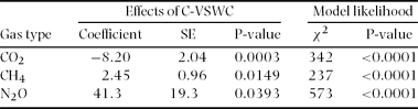
Temporal variation in CO2 flux was not related to that of soil C and N concentration (Table 2). Also, no significant relationship was observed between spatially averaged CO2 flux and spatially averaged C-VSWC across all sampling points (Figure 4a). Although no significant relationship was observed between C-VSWC and CH4 flux when considered for the entire period (Figure 4b), we found that the variation in negative CH4 flux was larger in dry periods (with a low C-VSWC) and became stable near zero in wetter periods (Figure 4b). Figure 4c shows a significant positive relationship (r = 0.97, P < 0.0005) between the spatially averaged N2O flux and C-VSWC at all sampling points on each sampling occasion. From the analysis by adjusting confounding effects of time, location and interaction between time and location in mixed models, C-VSWC has a negative effect on CO2 flux and positive effects on CH4 and N2O fluxes (Table 3).
Table 2. Pearson correlation coefficients and their levels of significance resulting from a regression between temporally averaged gas fluxes and the environmental factors monitored in the flux chambers on each sampling occasion (spatial variation) in Pasoh Forest Reserve of Peninsular Malaysia. All sampling occasions were divided into dry or wet periods (Figure 2b). The values of volumetric soil water content were measured at each flux chamber immediately after the flux measurement (C-VSWC). *P < 0.05, **P < 0.01, and ***P < 0.001.
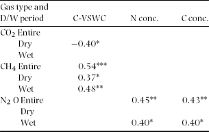

Figure 4. Relationships between the spatially averaged C-VSWC and spatially averaged CO2 flux of all sampling plots and of hot-spot points (HS1 and HS2) (a), CH4 flux (b) and N2O flux (c) in Pasoh Forest Reserve of Peninsular Malaysia. Error bars indicate SE.
Table 3. Effects of volumetric soil water content measured at each gas sampling chamber (C-VSWC) on each of the gas fluxes in Pasoh Forest Reserve of Peninsular Malaysia after adjusting for time, location and time-location interactions in repeated-measure mixed models
Spatial variation in GHG fluxes
When we classified all sampling times as dry, wet and entire periods, semivariogram analysis showed that CO2 flux had no spatial dependence and was randomly distributed in wet, dry, and entire periods (Table 1). As shown in Table 2, the spatial distribution of CO2 flux was not significantly related to any environmental factor other than the VSWC. Fine, coarse and total root biomass were not spatially related to CO2 flux for each sampling occasion. The spatial distribution of CO2 flux was significantly and negatively related to C-VSWC during dry periods (Table 2, Figure 5a). In contrast, no significant linear relationship was found during wet periods, or when using data for the entire period (Table 2, Figure 5a, b). In wet periods, extremely high CO2 emissions (>25 μmol CO2 m−2 s−1) were frequently observed at two sampling plots as shown in Figure 1c. These two plots, 15 and 13, referred to as HS1 and HS2, respectively, were referred as hot spots. Note that C-VSWC values at these two hot spots were not very high and were lower than saturated conditions (WFPS: 57.5–83.0%) even during wet periods (Figure 5a, b).

Figure 5. Relationships between the temporally averaged C-VSWC and temporally averaged CO2 flux(a), CH4 flux (b) and N2O flux (c) during dry/wet periods, and between the temporally averaged C-VSWC and CO2 flux(d), CH4 flux (e), and N2O (f) flux during entire sampling period in the Pasoh Forest Reserve of Peninsular Malaysia. Error bars indicate SE.
The semivariograms of CH4 flux showed moderate spatial dependency only in wet periods, the ranges and sills observed were not precisely determined because the ranges were more than the effective range (Table 1). For dry and entire periods, CH4 flux had no spatial dependence. Among the environmental factors, C-VSWC showed the best correlation with the spatial variation in CH4 flux for the dry, wet and entire period (Table 2, Figure 5c, d). However, larger CH4 emissions (> 5 mg CH4 m−2 d−1; as high as 17.9 mg CH4 m−2 d−1 in March 2007) were occasionally observed in dry periods (Figure 5c), which obscured the linear relationship between CH4 flux and C-VSWC for dry periods. Temporally averaged CH4 flux for all sampling points was not significantly related to those of soil N and C concentrations (Table 2).
N2O flux had spatial dependence in wet, dry and entire periods with Q values of 0.84, 0.98 and 0.83 and ranges of 39.9, 40.1, 39.9 m, respectively (Table 1). Although spatial variation in N2O showed no significant relationship to C-VSWC for both dry and wet periods, a significant positive relationship was revealed when the entire study period's data were considered (Table 2, Figure 5e, f). As for soil N concentration, the spatial variation in N2O flux was significantly related to that of soil N concentration for wet periods and the entire period (P < 0.001; Table 2, Figure 6a, b). In contrast, in dry periods, N2O emissions were significantly lower than in wet periods, even at sampling points with high soil N concentrations. These dry-period patterns resulted in no significant relationship between N2O flux and soil N concentration (Table 2, Figure 6a). Temporally averaged N2O flux was the highest at point 11, where the soil N2O concentration was the highest at deeper (30 and 50 cm) depths (of the five sampling points, data not shown), and C-VSWC and soil C and N concentrations were also high.

Figure 6. Relationships between the temporally averaged soil N concentration and temporally averaged N2O flux during dry/wet periods (a) and during entire sampling period (b) in the Pasoh Forest Reserve of Peninsular Malaysia. Error bars indicate SE.
DISCUSSION
CO2 flux
Mean CO2 flux in this study was lower than those reported from Amazonian tropical rain forest sites (mean: 6.45 μmol CO2 m−2 s−1; Doff Sotta et al. Reference DOFF SOTTA, MEIR, MALHI, NOBRE, HODNETT and GRACE2004) and that of Borneo, Malaysia (mean 5.7 ± 1.9 (SD) μmol CO2 m−2 s−1; Katayama et al. Reference KATAYAMA, KUME, KOMATSU, OHASHI, NAKAGAWA, YAMASHITA, OTSUKI, SUZUKI and KUMAGAI2009), consistent with tropical rain forests in French Guiana (mean: 4.26 μmol CO2 m−2 s−1; Epron et al. Reference EPRON, BOSC, BONAL and FREYCON2006) and higher than those of Indonesian primary forests (mean: 1.47 or 2.17 μmol CO2 m−2 s−1; Ishizuka et al. Reference ISHIZUKA, TSURUTA and MURDIYARSO2002) and a Kenyan rain forest (range: 1.36–2.04 μmol CO2 m−2 s−1; Werner et al. Reference WERNER, KIESE and BUTTERBACH-BAHL2007).
The lack of significant relationships between the temporal variation in CO2 flux and either soil C or N concentration implies that the temporal variation in soil C and N concentrations (2.6–4.5% and 0.21–0.31%, respectively) at our study site were not driving soil CO2 flux. As for soil water status, Kosugi et al. (Reference KOSUGI, MITANI, ITOH, NOGUCHI, TANI, MATSUO, TAKANASHI, OHKUBO and RAHIM2007) reported a significant positive relationship between temporal variation of CO2 flux and VSWC for a smaller area than ours (50 × 50 m plot). Results from other tropical rain-forest sites also showed positive relationships (Butterbach-Bahl et al. Reference BUTTERBACH-BAHL, KOCK, WILLIBALD, HEWETT, BUHAGIAR, PAPEN and KIESE2004; Davidson et al. Reference DAVIDSON, KELLER, ERICKSON, VERCHOT and VELDKAMP2000a; Werner et al. Reference WERNER, KIESE and BUTTERBACH-BAHL2007). Some of these results suggest that continuing wet periods stimulate respiration. In contrast, Schwendenmann et al. (Reference SCHWENDENMANN, VELDKAMP, BRENES, O'BRIEN and MACKENSEN2003) reported a parabolic relationship between soil water content and seasonal variation in soil respiration rates. They suggested that CO2 emissions were reduced due to lower diffusion rates under conditions of high soil water content. In our case, neither significant positive nor negative relationships were observed between spatially averaged CO2 flux and C-VSWC if we do not consider the interaction between time and space.
Some environmental factors controlling the spatial variation in CO2 flux have been reported previously at our study site, such as fine-root biomass (Adachi et al. Reference ADACHI, BEKKU, RASHIDAH, OKUDA and KOIZUMI2006) and soil N content (Kosugi et al. Reference KOSUGI, MITANI, ITOH, NOGUCHI, TANI, MATSUO, TAKANASHI, OHKUBO and RAHIM2007). However, the spatial distribution of CO2 flux in this study was not significantly related with soil N content, except during the dry period (Table 2). This may be attributed to spatial dependence of N content except dry period with range of 96.7 (wet period) and 37.2 m (entire period; Table 1). When we classified all sampling times as dry, wet and entire periods, a significant relationship between the spatial distribution of CO2 flux and C-VSWC was found only for the dry period (Table 2). However, CO2 flux was certainly affected by C-VSWC with eliminating the confounding effects of time, location and interaction between them (Table 3). Such a significant negative relationship between CO2 flux and C-VSWC gave similar results to those from the two previous studies. A decrease in gas diffusivity with high wet-period VSWC probably contributed to low O2 concentrations that inhibited aerobic microbial activity (Davidson et al. Reference DAVIDSON, BELK and BOONE1998, Linn & Doran Reference LINN and DORAN1984). During the wet period, however, higher CO2 emissions occasionally occurred at hot spots, which obscured any significant relationships (thus none was found).
Considering that much higher soil CO2 concentrations occurred in wet periods (Figure 3a), our results imply that correspondingly high CO2 emissions during wet periods were partly due to CO2 displacement in the soil through the preferential flow of rainwater (Singh & Gupta Reference SINGH and GUPTA1977). Noguchi et al. (Reference NOGUCHI, ABDUL RAHIM, KASRAN, TANI, SAMMORI and MORISADA1997) found in other Peninsular Malaysia tropical rain-forest sites that decayed and even living roots can provide vertical channels that act as pipes to affect preferential water flow paths. Tunnel networks excavated by termites may also serve as a macropore water-transfer system (Matsumoto et al. Reference MATSUMOTO, IKEDA and SHINDO1991). The preferential flow of high concentrations of soil CO2 through these pores during the wet period (Figure 3) may cause high emissions from the soil surface. Also, we cannot rule out CO2 emissions from animal respiration. Among the few studies that explored the spatial distribution of CO2 emissions in tropical rain forests, Ohashi et al. (Reference OHASHI, KUME, YAMANE and SUZUKI2007) suggested that CO2 hot spots may represent as much as 10% of the total soil respiration and that they are possibly the contribution of animal activity (e.g. termites and ants). Such hot-spot emissions were also reported in tropical rain forests of the Brazilian Amazon (Davidson et al. Reference DAVIDSON, KELLER, ERICKSON, VERCHOT and VELDKAMP2000a) and Thailand (Hashimoto et al. Reference HASHIMOTO, TANAKA, SUZUKI, INOUE, TAKIZAWA, KOSAKA, TANAKA, TANTASIRIN and TANGTHAM2004). Hot-spot CO2 emissions observed at HS1 and HS2 during the wet period (Table 2) contributed to both the large variation and weak correlation in a regression plot of C-VSWC vs. CO2 flux. Moreover, CO2 emissions observed at hot-spots (HS1 and HS2) showed a temporary significant positive correlation with the VSWC (Figure 4a; r = 0.91, P < 0.001). These flux might be related to termite activity with previous reports of Matsumoto (Reference MATSUMOTO1976) and Yamada et al. (Reference YAMADA, INOUE, WIWATWITAYA, OHKUMA, KUDO, ABE and SUGIMOTO2005) which showed the importance of termites on carbon mineralization and of Brümmer et al. (Reference BRÜMMER, PAPEN, WASSMANN and BRÜGGEMANN2009) showing that CO2 emissions from termites peak at soil temperatures of below 32 °C and soil moisture above 60%. Such hot-spot emission of CO2 may attribute to lack of spatial dependence of CO2 flux in our site (Table 1). In the future, to clarify large spatial and temporal variations of CO2 flux in the wet period, more information is needed for both biological and geographical characteristics. Recently, Katayama et al. (Reference KATAYAMA, KUME, KOMATSU, OHASHI, NAKAGAWA, YAMASHITA, OTSUKI, SUZUKI and KUMAGAI2009) reported significant positive correlation between the soil respiration and forest structural parameters such as the mean diameter at breast height (dbh), suggesting that the effects of spatial distribution of emergent trees should be taken into account. In addition to the report, our results suggest that considering the effects of decomposer activities may help to explain the complex temporal and spatial patterns in CO2 flux.
CH4 flux
Our results showed that the soil at this site functioned as a small net sink for CH4. The mean value of CH4 flux observed at our site was consistent with the results from an Australian tropical rain forest (mean: −0.76 mg CH4 m−2 d−1; Butterbach-Bahl et al. Reference BUTTERBACH-BAHL, KOCK, WILLIBALD, HEWETT, BUHAGIAR, PAPEN and KIESE2004) and Indonesian primary forests (mean: −0.67 and 0.13 mg CH4 m−2 d−1 for two observation sites; Ishizuka et al. Reference ISHIZUKA, TSURUTA and MURDIYARSO2002), and larger (lower uptake) than a Kenyan rain forest (range: −2.82 to −1.25 mg CH4 m−2 d−1; Werner et al. Reference WERNER, KIESE and BUTTERBACH-BAHL2007).
The significant positive relationship between spatial variation in CH4 flux and C-VSWC for the dry, wet and entire period (Figure 5c, d) indicated that the spatial distribution of CH4 flux is mainly controlled by soil water condition. If we eliminate the confounding effects of time, location and interaction between them (Table 3), CH4 flux was certainly affected by C-VSWC. Blankinship et al. (Reference BLANKINSHIP, BROWN, DIJKSTRA, ALLWRIGHT and HUNGATE2010) reported that increased and reduced precipitation treatments decreased and increased, respectively, CH4 uptake in the mixed conifer forest mesocosm. Itoh et al. (Reference ITOH, OHTE and KOBA2009) found that CH4 production in periods of high temperature can exceed CH4 oxidation, even in unsaturated temperate forest soils of the Asian monsoon region. They indicated that CH4 emissions in the high VSWC range might be due to increased methanogen activity. Also, high soil gas CH4 concentrations were observed during the wettest period (Figure 3b), especially at points 1 and 11 where the soil was wetter than at other points. These support the idea that CH4 was produced under anaerobic conditions. This corresponds with previous reports from Australian tropical rain forests (Kiese et al. Reference KIESE, HEWETT, GRAHAM and BUTTERBACH-BAHL2003), suggesting that a higher CH4 flux during wetter periods is attributable to CH4 production under continuing wet soil conditions. Alternatively, the limitation of CH4 oxidation due to the lower gas diffusivity in wet periods (Born et al. Reference BORN, DÖRR and LEVIN1990, Dörr et al. Reference DÖRR, KATRUFF and LEVIN1993) may also have affected the positive relationship between VSWC and CH4 flux.
Moderate spatial dependence of CH4 flux and VSWC in wet periods (Table 1) suggests that the spatial variation in CH4 flux at our site was mainly affected by VSWC especially for wet periods. In contrast, no spatial dependence of CH4 flux in dry periods (Table 1) may be due to sporadic large CH4 emissions (e.g. March 2007). These high CH4 emissions were usually observed together with low-VSWC, when CH4 production by methanogenesis does not usually occur in forest soil. Considering that the study site was reportedly rich in termite species (Abe & Matsumoto Reference ABE and MATSUMOTO1979, Matsumoto Reference MATSUMOTO1976), we assume that CH4 production may have increased as a result of aerobic termite activity in dry periods (Sugimoto et al. Reference SUGIMOTO, INOUE, TAYASU, MILLER, TAKEICHI and ABE1998a, Reference SUGIMOTO, INOUE, KIRTIBUTR and ABE1998b). On 7 March 2007, we also collected gas samples from the mounds of Dicuspiditermes sp. during the flux measurement. We found that CH4 concentrations in the mounds were relatively high, which registered 6.5 ppmv at a depth of 10 cm, 37.7 ppmv at 20 cm and 17.4 ppmv at 30 cm. Furthermore, many publications have reported that worker termites produce CH4, from trace amounts up to 1.6 μmol g−1 h−1 (Nunes et al. Reference NUNES, BIGNELL, LO and EGGLETON1997, Sugimoto et al. Reference SUGIMOTO, INOUE, KIRTIBUTR and ABE1998a). However, Sanderson (Reference SANDERSON1996) reported that the contribution of CH4 by termites to global climate is minimal since the gross production by termites is below 20% of all global sources, with net production as low as 1% or less.
As a whole, even though hot spots due to termite activity may obscure the relationship between CH4 flux and environmental factors and should be considered in the future, our results indicate that spatial variation in CH4 flux in our site was controlled mainly by spatial variation in the soil water status for the entire period of this study.
N2O flux
N2O flux at our study site was much larger than those reported for an Australian tropical rain forest (range: 0–101 μg N m−2 h−1, mean: 25.6 μg N m−2 h−1; Butterbach-Bahl et al. Reference BUTTERBACH-BAHL, KOCK, WILLIBALD, HEWETT, BUHAGIAR, PAPEN and KIESE2004), an Indonesian primary forest (mean: 1.47 or 4.43 μg N m−2 h−1; Ishizuka et al. Reference ISHIZUKA, TSURUTA and MURDIYARSO2002), and a Kenyan rain forest (range: 1.1–325 μg N m−2 h−1, mean: 42.9 μg N m−2 h−1; Werner et al. Reference WERNER, KIESE and BUTTERBACH-BAHL2007).
When we eliminate the confounding effects of time, location and interaction between them, N2O flux was positively affected by C-VSWC (Table 3). Segregation of sampling times into dry, wet and entire period suggest that, spatially, N2O flux was highest where high VSWC values were maintained throughout the entire sampling period. These significant positive relationships between N2O flux and C-VSWC indicate that N2O flux was controlled by variation in soil water conditions at a longer temporal scale than each dry or wet period, and that the range of such temporal variation was much wider than the range of spatial variation in each dry and wet period. Spatial variation in N2O flux was also positively related to soil N concentration for both the wet and the entire period. However, segregation and analysis of just the dry period did not reveal such a relationship. These results suggest that the spatial distribution of N2O flux was controlled by both VSWC and soil N concentration, which must be related to available N sources for both nitrification and denitrification. Spatial dependences of N2O flux and soil N contents within almost the same ranges (N2O, 39.9 m; soil N, 37.2 m) in wet period and high soil gas N2O concentrations observed at point 11, especially during wet periods, also support this idea.
The question remains whether N2O emissions are caused by nitrification or denitrification. As reported by Bateman & Baggs (Reference BATEMAN and BAGGS2005), at lower soil water contents such as 35–60% WFPS, nitrification is considered to be the main process producing N2O. Some reports have shown a relationship between soil nitrification rate and N2O flux from tropical soils (as summarized by Ishizuka et al. Reference ISHIZUKA, TSURUTA and MURDIYARSO2002), suggesting that nitrification is a main factor in N2O emissions at such sites. However, these sites had much lower N2O flux than our site (maximum: 40 μg N m−2 h−1) under almost the same soil N conditions. Meanwhile, denitrification becomes increasingly dominant at >60% WFPS, i.e. under conditions in which soils are becoming predominantly anaerobic (Davidson et al. Reference DAVIDSON, KELLER, ERICKSON, VERCHOT and VELDKAMP2000b, Linn & Doran Reference LINN and DORAN1984). Additionally, Davidson et al. (Reference DAVIDSON, MATSON, VITOUSEK, RILEY, DUNKIN, GARCÍA-MÉNDEZ and MAASS1993) suggested that denitrification was the dominant source of N2O during the wet season in a dry tropical forest in Mexico. Although we do not have detailed data such as inorganic N soil fraction, a large N2O emission pulse was observed only in the wet period and at points with high soil N concentrations at our site. A significant positive relation of the spatially averaged N2O flux to that of C-VSWC indicate that temporal variation of N2O flux was controlled by temporal variation of soil water status. During the wettest period of sampling, the WFPS was 76.0% (range: 52.9–100%; 12 December 2007) and 70.7% (47.1–96.7%; 16 December 2007) in the top 0–5 cm of soil. These values may be high enough to allow denitrification to dominate (Davidson et al. Reference DAVIDSON, KELLER, ERICKSON, VERCHOT and VELDKAMP2000b). Under such wet conditions, we recorded individual N2O flux as high as 3132 μg N m−2 h−1. This value was much higher than any other reports from tropical rain forests (maximum 324.8 μg N m−2 h−1 in Werner et al. Reference WERNER, KIESE and BUTTERBACH-BAHL2007, 492.1 μg N m−2 h−1 in Breuer et al. Reference BREUER, PAPEN and BUTTERBACH-BAHL2000, and 570.8 μg N m−2 h−1 in Kiese & Butterbach-Bahl Reference KIESE and BUTTERBACH-BAHL2002). These correspond with results from other reports (Butterbach-Bahl et al. Reference BUTTERBACH-BAHL, KOCK, WILLIBALD, HEWETT, BUHAGIAR, PAPEN and KIESE2004, Davidson et al. Reference DAVIDSON, ISHIDA and NEPSTAD2004, Werner et al. Reference WERNER, KIESE and BUTTERBACH-BAHL2007), suggesting that denitrification was the main process causing high N2O emission at our site.
As a concluding remark, we found that soil water status was related to rainfall and controlled greenhouse gas (GHG) fluxes from the soil at the study site via several biogeochemical processes, including gas diffusion and soil redox conditions. Our results also suggest that considering the biological effects such as decomposer activities may help to explain the complex temporal and spatial patterns in CO2 and CH4 fluxes.
ACKNOWLEDGEMENTS
We thank the editor and anonymous reviewer for valuable comments on an earlier draft of this manuscript; the Forestry Department of Negeri Sembilan and the Director General of the Forest Research Institute Malaysia (FRIM) for granting us permission to work in the Pasoh Forest Reserve. We also thank a joint research project between FRIM, Putra University, Malaysia (UPM), and the National Institute for Environmental Studies (NIES), Japan. We additionally thank Drs S. Sudo, N. Matsuo, K. Tanaka, T. Nakaji and M. Dannoura, N. Makita, and Mr. R. Nakagawa and A. Kanazawa for their help with gas flux measurements and K. Nishina, K. B. Neoh and T. Furusawa for valuable comments. This work was supported by Grants-in-Aid for Scientific Research, Japan and by the program ‘Southeast Asia Studies for Sustainable Humanosphere’, MEXT, Japan.


