


1. Introduction
In hypersonic flight of a vehicle, the temperature downstream of the bow shock is high enough to cause the molecular components of the atmosphere to become vibrationally excited and to dissociate. This introduces two new phenomena: the equilibrium equation of state is changed, and the finite rates at which the vibrational excitation and dissociation proceed – collectively referred to as relaxation effects – add new length scales.
Such high-enthalpy real-gas effects can cause important changes to flight characteristics of hypersonic vehicles. For example, a near-disastrous situation was encountered during the first space shuttle flight in which they influenced the longitudinal stability of the vehicle to the limit of the elevator flap deflection, see e.g. Maus et al. (Reference Maus, Griffith, Szema and Best1984). This emphasizes the importance of perfecting ground testing and computational tools to enable precise design procedures.
While the equilibrium behaviour of gases at high temperature can be determined very accurately from theory, see e.g. Gordon & McBride (Reference Gordon and McBride1994), the rates of vibrational excitation and dissociation have required complex measurements in shock tubes and other devices, although recent developments employing sophisticated theoretical methods to obtain the relevant data have been quite successful, see e.g. Macdonald et al. (Reference Macdonald, Torres, Schwartzentruber and Panesi2020) and Chaudry et al. (Reference Chaudry, Boyd, Torres, Schwartzentruber and Candler2020). Nevertheless, the uncertainties associated with dissociation rates remain so high that they are usually quoted as error margins of  $\pm$0.2 or so in the power of 10.
The manifestations of finite rates in practical flows are often not very apparent. However, this is not universally the case, and there are some particular flows where they cause major changes. One of these is the location of a half-saddle point in the density field downstream of a curved bow shock, which has been shown to be very sensitive to the relaxation rate by Hornung (Reference Hornung2010) and confirmed by Candler (Reference Candler2010). However, experimental determination of this location requires field measurements such as optical interferometry.
Another is the detachment distance of the bow shock in symmetrical flow over a wedge. It was predicted on theoretical grounds by Hornung & Smith (Reference Hornung and Smith1979) that, in the range of wedge angles between the frozen (zero rates) and equilibrium detachment angles, the detachment distance is scaled by the relaxation length rather than by the geometric dimensions of the wedge. They followed up their prediction with a convincing experimental confirmation in high-enthalpy nitrogen and carbon dioxide flows performed in the T3 free-piston driven reflected shock tunnel. Much of this work was done by G. Smith for his fourth year honours thesis in the Physics Department of the Australian National University at Canberra. His thesis details meticulous records of the experiment that provide important input for our work.
A schematic sketch of two-dimensional flow over a wedge is shown in figure 1 in the non-relaxing and in the relaxing situation. This sketch defines the geometrical parameters wedge flank length  $w$, wedge angle
  $\theta$, shock stand-off distance
  $\varDelta$ and wedge height
  $H$. The real case of the experiment is, of course, three-dimensional. This introduces the length
  $L$ of the model in the transverse direction.
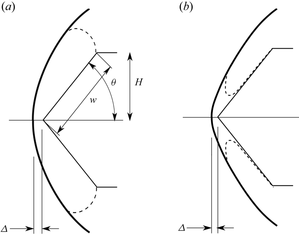
Figure 1. Schematic sketches of wedge flow with detached shock. (a) Perfect-gas or equilibrium flow showing definition of geometrical parameters. The sonic line is shown as a dashed line. (b) Relaxing flow in the range of wedge angles between the frozen and equilibrium detachment angles; note new location of the sonic line.
The experiments of Hornung & Smith (Reference Hornung and Smith1979) have been examined by two-dimensional computations, e.g. by Bondar et al. (Reference Bondar, Markelov, Gimelshein and Ivanov2005), who found only marginal agreement. However, since the transverse length  $L$ of the wedge in the experiment is only three times as large as the flank length
  $w$, it is clear that any computation to be compared with the experiment must be made in three dimensions.
The main aim of the present work is to compare the results of Hornung & Smith (Reference Hornung and Smith1979) with three-dimensional computations. However, to set the scene, the effect of relaxation on shock detachment is first discussed using two-dimensional computations of non-equilibrium nitrogen flow. Next, three-dimensional computations of ideal-gas and thermally perfect flows will be used to attempt to extend the powerful analytical expressions recently obtained for non-relaxing flow by Hornung (Reference Hornung2021) for  $\varDelta /w$, to three dimensions. Finally, three-dimensional non-equilibrium computations of nitrogen and carbon dioxide flows will be made at the conditions of the experiment.
1.1. Notation
We take  $x$,
$x$,  $y$ and
  $z$ as the streamwise, normal and spanwise coordinates with corresponding velocity components
  $u$,
$u$,  $v$ and
  $w$. The spanwise length of the wedge is
  $L$, and
  $p$,
$p$,  $\rho$,
  $T$ and
  $T_v$ denote pressure, density, translational and vibrational temperature;
  $M$ and
  $\gamma$ denote Mach number and specific heat ratio. The species mass fraction vector is denoted by
  $\boldsymbol {c}$ and its components are identified by their chemical formula as subscripts, e.g.
  $c_{N_2}$. The subscript
  $\infty$ is used to define free-stream values. The wedge angle
  $\theta _d$ is the value of
  $\theta$ above which the shock wave is detached.
2. Computational tools and implementation
The Eilmer flow simulation software is a derivative of the Navier–Stokes solver described by Jacobs (Reference Jacobs1991). It has been further developed over the years, especially for high-temperature hypersonic flows, and with some significant effort toward verification by Gollan & Jacobs (Reference Gollan and Jacobs2013). The description of the Eilmer code in this section is limited to the formulation of the inviscid gas dynamics, together with the thermal and chemical non-equilibrium modelling, since these are of primary interest in this study. A more complete description, including the handling of viscous effects, is available in Gibbons et al. (Reference Gibbons, Damm, Gollan and Jacobs2022).
2.1. Conservation equations
Eilmer is formulated around the integral form of the conservation equations, which can be written as
 \begin{equation} \frac{\partial}{\partial t} \int_{V} U \,{\rm d}V ={-} \oint_{S} \left ( \bar{F}_{c} - \bar{F}_{v} \right )\, {\cdot}\, \hat{n}\,{\rm d}A + \int_{V} Q\,{\rm d}V , \end{equation}
where  $S$ is the bounding surface and
  $\hat {n}$ is the outward-facing unit normal of the control surface. The symbol
  $V$ in (2.1) is the volume of a cell while
  $A$ is the area of the cell boundary. For a gas in thermal and chemical non-equilibrium governed by two temperatures, the vector of conserved quantities carried in a simulation is
 \begin{equation} U = \left [
\begin{array}{@{}c@{}} \rho \\ \rho v_{x} \\ \rho v_{y} \\ \rho
v_{z} \\ \rho E \\ \vdots \\ \rho_{s} \\ \vdots \\ \rho
e_{v} \end{array} \right ],
\end{equation}
\begin{equation} U = \left [
\begin{array}{@{}c@{}} \rho \\ \rho v_{x} \\ \rho v_{y} \\ \rho
v_{z} \\ \rho E \\ \vdots \\ \rho_{s} \\ \vdots \\ \rho
e_{v} \end{array} \right ],
\end{equation}
where the conserved quantities are respectively density,  $x$-,
$x$-,  $y$- and
  $z$-momentum per volume, total energy per volume, followed by
  $n_{sp}$ individual densities for the chemical species and the mixture vibroelectronic energy per volume.
The flux vectors are divided into convective and viscous-transport contributions. With the specific internal energy of the gas being  $e$ and the total specific energy being
  $E = e + v^2/2$, the convective component is
 \begin{equation} \bar{F}_{c} = \begin{bmatrix} \rho v_{x} \\ \rho v_{x}^{2} + p \\ \rho
v_{x} v_{y} \\ \rho v_{x} v_{z} \\ \rho E v_{x} + p v_{x}
\\ \vdots \\ \rho_{s} v_{x} \\ \vdots \\ \rho e_{v} v_{x}
\\ \end{bmatrix} \hat{i} + \begin{bmatrix}
\rho v_{y} \\ \rho v_{y} v_{x} \\ \rho v_{y}^{2} + p \\
\rho v_{y} v_{z} \\ \rho E v_{y} + p v_{y} \\ \vdots \\
\rho_{s} v_{y} \\ \vdots \\ \rho e_{v} v_{y} \\ \end{bmatrix}
\hat{j} + \begin{bmatrix} \rho v_{z} \\
\rho v_{z} v_{x} \\ \rho v_{z} v_{y} \\ \rho v_{z}^{2} + p
\\ \rho E v_{z} + p v_{z} \\ \vdots \\ \rho_{s} v_{z} \\
\vdots \\ \rho e_{v} v_{z} \\ \end{bmatrix} \hat{k}
. \end{equation}
\begin{equation} \bar{F}_{c} = \begin{bmatrix} \rho v_{x} \\ \rho v_{x}^{2} + p \\ \rho
v_{x} v_{y} \\ \rho v_{x} v_{z} \\ \rho E v_{x} + p v_{x}
\\ \vdots \\ \rho_{s} v_{x} \\ \vdots \\ \rho e_{v} v_{x}
\\ \end{bmatrix} \hat{i} + \begin{bmatrix}
\rho v_{y} \\ \rho v_{y} v_{x} \\ \rho v_{y}^{2} + p \\
\rho v_{y} v_{z} \\ \rho E v_{y} + p v_{y} \\ \vdots \\
\rho_{s} v_{y} \\ \vdots \\ \rho e_{v} v_{y} \\ \end{bmatrix}
\hat{j} + \begin{bmatrix} \rho v_{z} \\
\rho v_{z} v_{x} \\ \rho v_{z} v_{y} \\ \rho v_{z}^{2} + p
\\ \rho E v_{z} + p v_{z} \\ \vdots \\ \rho_{s} v_{z} \\
\vdots \\ \rho e_{v} v_{z} \\ \end{bmatrix} \hat{k}
. \end{equation}
Although the viscous components,  $F_{v}$, are available in the Eilmer code, they are not a major player in the present study.
The vector of source terms includes the species rates of reaction and thermal energy exchanges, which are discussed in the following section
 \begin{equation} Q = \begin{bmatrix} 0 \\ 0 \\ 0 \\ 0 \\ 0 \\ \vdots \\ M_s
\dfrac{{\rm d}[X_s]}{{\rm d}t} \\ \vdots \\
Q^{{vib\text{-}trans}} + Q^{{vib\text{-}chem}}\end{bmatrix}. \end{equation}
\begin{equation} Q = \begin{bmatrix} 0 \\ 0 \\ 0 \\ 0 \\ 0 \\ \vdots \\ M_s
\dfrac{{\rm d}[X_s]}{{\rm d}t} \\ \vdots \\
Q^{{vib\text{-}trans}} + Q^{{vib\text{-}chem}}\end{bmatrix}. \end{equation}
2.2. Equations of state and thermodynamic properties
The governing equations are closed using equations of state. In this work, a two-temperature model is used to account for thermochemical non-equilibrium. The two temperatures are a transrotational temperature,  $T$, and a vibroelectronic temperature,
  $T_v$. The thermal equation of state for the pressure of the gas mixture is obtained from Dalton's law of partial pressures. Each component in the mixture is assumed to obey the ideal-gas law (perfectly elastic collisions of point particles). The pressure for a mixture of
  $n_{sp}$ species is
 \begin{equation} p = \sum_{s=1}^{n_{sp}} \rho_s R_s T, \end{equation}
where  $\rho _s$ is the partial density of species
  $s$,
$s$,  $R_s$ is the specific gas constant of species
  $s$ and
  $T$ is the transrotational temperature.
The caloric equation of state relates the internal energy of the mixture to the temperatures in the gas. The mixture energy is expressed as a mass fraction weighted contribution from the internal energy of each component species as
 \begin{equation} e = \sum_{s=1}^{n_{sp}} c_s e_s(T, T_v). \end{equation}
 The calculation of  $e_i$ closely follows the approach described in the two-temperature model presented in Gnoffo, Gupta & Shinn (Reference Gnoffo, Gupta and Shinn1989). That approach is described here. It is convenient to work with specific heat,
  $C_p$, and enthalpy,
  $h$, since thermodynamic curve fits are commonly available in these forms.
The two-temperature gas model used in this work assumes one Boltzmann distribution of translation and rotational energy levels described by  $T$, and a second Boltzmann distribution of vibrational and electronic energy levels described by
  $T_v$. Under this assumption, the specific heat at constant pressure for species
  $s$ is
 \begin{equation} C_{p,s}(T, T_v) = C_{p_t,s}(T) + C_{p_r,s}(T) + C_{p_{v e},s}(T_v) . \end{equation}
For atomic species, there is no appreciable energy storage in rotational modes, so  $C_{p_r,{atoms}} = 0$. The vibroelectronic energy storage has been grouped in one term,
  $C_{p_{v e}}$. Note that storage in the electronic mode is small enough to be negligible at the temperatures of interest in this work. However, it is included here because it is faithful to the implementation used for the simulations.
Curve fits are available for  $C_p$ for individual species as a function of a single temperature. They are valid under an assumption of thermal equilibrium. However, these curve fits are convenient to use to compute the vibrational and electronic contributions to
  $C_p$ because the translational and rotational contributions are constant. These contributions are constant because these modes are assumed to be fully excited at the temperatures of interest for this work. Here, we use the equilibrium curve fits and data from the Chemical Equilibrium Applications program of Gordon & McBride (Reference Gordon and McBride1994), which has the form
 \begin{equation} C_{p,s}(T) = R_s (a_0 T^{{-}2} + a_1 T^{{-}1} + a_2 + a_3 T + a_4 T^2 + a_5 T^3 + a_6 T^4). \end{equation}
For all particles, under the assumption of fully excited translation
 \begin{equation} C_{p_t,s} = \frac{5}{2} R_s. \end{equation}
For linear molecules (N $_2$, O
 $_2$, CO) with fully excited rotation
 \begin{equation} C_{p_r,s} = R_s \end{equation}
and for nonlinear molecules (here: CO $_2$)
$_2$)
 \begin{equation} C_{p_r,s} = \frac{3}{2} R_s. \end{equation}
These constant contributions can be subtracted from (2.8) to compute the vibroelectronic specific heat as
 \begin{equation} C_{p_{iv e},s}(T_v) = C_{p,s}(T_v) - C_{p_t,s} - C_{p_r,s}. \end{equation}
 The calculation of enthalpy for each species follows the same idea as  $C_p$, that is, use a curve fit for enthalpy assuming thermal equilibrium and then subtract out the fully excited modes. The idea is shown here in equation form. The curve fits for enthalpy at thermal equilibrium following Gordon & McBride (Reference Gordon and McBride1994) are
 \begin{align} h_s(T) = (R_sT) \left({-}a_0 T^{{-}2} + a_1 T^{{-}1} \log{T} + a_2 + a_3 \frac{T}{2} + a_4 \frac{T^2}{3} + a_5 \frac{T^3}{4} + a_6 \frac{T^4}{5} + \frac{a_7}{T} \right). \end{align}
The constant  $a_7$ in (2.13) represents a reference enthalpy,
  $h_{{ref.}}$, which for the Gordon & McBride (Reference Gordon and McBride1994) curves is taken as the enthalpy of formation at 298.15 K. Using these curve fits, the vibroelectonic enthalpy is computed as
 \begin{equation} h_{v e,s}(T_v) = h_s(T_v) - (C_{p_t,s} + C_{p_r,s})(T_v - T_{{ref.}}) - h_{{ref.},s}. \end{equation}
The enthalpy in species  $s$ including all energy mode contributions is computed as
 \begin{equation} h_s(T, T_v) = (C_{p_t,s} + C_{p_r,s})(T - T_{{ref.}}) + h_{v e,s}(T_v) + h_{{ref.},s}. \end{equation}
As a final step, the energy in species  $s$ is (assuming the ideal-gas law)
 \begin{equation} e_s(T, T_v) = h_s - R_sT. \end{equation}
2.3. Chemistry modelling in thermal non-equilibrium
The chemistry source term is computed using the law of mass action. A collection of simple reversible reactions can be represented by
 \begin{equation} \sum_{s=1}^{n_f} \alpha_s X_s \rightleftharpoons \sum_{s=1}^{n_b} \beta_s X_s, \end{equation}
where  $\alpha _s$ and
  $\beta _s$ represent the stoichiometric coefficients for the reactants and products respectively, and
  $X_s$ represents gaseous species
  $s$. For a given reaction
  $r$, the rate of concentration change of species
  $s$ is given as,
 \begin{equation} \left( \frac{{\rm d}[X_s]}{{\rm d}t} \right)_r = \nu_s \left\{ k_f \prod_i [X_i]^{\alpha_i} - k_b \prod_i [X_i]^{\beta_i} \right\}, \end{equation}
where  $\nu _s = \beta _s - \alpha _s$. By summation over all reactions,
  $n_r$, the total rate of concentration change is
 \begin{equation} \frac{{\rm d}[X_s]}{{\rm d}t} = \sum_{r=1}^{N_r} \left( \frac{{\rm d}[X_s]}{{\rm d}t} \right)_r. \end{equation}
 The chemical rate equations require rate constants,  $k_{f,r}$ and
  $k_{b,r}$, for the forward and backward rates of each reaction. These are computed using the generalized Arrhenius form based on a rate-controlling temperature,
  $T_a$,
 $$\begin{gather} k_{f,r} = A T_a^{n} \exp{\left( \frac{-C}{T_a}\right)}, \end{gather}$$
 $$\begin{gather}k_{b,r} = A T_a^{n} \exp{\left(\frac{-C}{T_a}\right)}, \end{gather}$$
or when  $k_{b,r}$ rate constant data are unavailable, it is computed using the forward rate constant and the concentration equilibrium constant as
 \begin{equation} k_{b,r} = \frac{k_{f,r}}{K_{c,r}(T)}. \end{equation}
 To account for the effect of thermal non-equilibrium – in this case, we mean specifically vibrational non-equilibrium – a model is used to modify the chemical reaction rates. In this work, the two-temperature model of Park (Reference Park1988) is used. In this model, Park proposes that a weighted average of the translation and vibrational temperatures be used for the rate-controlling temperature in computing forward rate constants involving molecular species. The expression for rate-controlling temperature  $T_a$ is
 \begin{equation} T_a = T^s T_v^{1-s}, \end{equation}
where  $s$ is a parameter of the model and is taken as a value between 0.5 and 0.7. The parameter
  $s$ is usually calibrated against experiment. For a time, it was accepted practice to set
  $s = 0.5$ in expanding flows and
  $s = 0.7$ in compressive flows. However, more recently in Park (Reference Park2010), the conclusion is that there has been no clear demonstration of any advantage of using 0.7 over 0.5. In the simulations of this work, we use
  $s = 0.5$. Thus the rate-controlling temperature is a geometric average of the translational and vibrational temperatures,
  $\sqrt {TT_v}$.
In the simulations involving nitrogen, presented later, chemical rate constant parameters have been taken from two sources: Kewley & Hornung (Reference Kewley and Hornung1974) and Park (Reference Park1993). For the simulation with a carbon dioxide mixture, the reaction rates from Ebrahim & Hornung (Reference Ebrahim and Hornung1973) are used. All of the reaction rate parameters are given in the Appendix in tables 4–6.
2.4. Energy exchange models
The energy exchange source terms in (2.4) account for the exchange of energy between the vibroelectronic and transrotational modes,  $Q^{{vib\text {-}trans}}$, and the energy change in the vibroelectronic mode due to chemistry effects,
  $Q^{{vib\text {-}chem}}$.
The Landau–Teller model is used to compute the energy exchange between the vibroelectronic and transrotational modes. The model uses the assumption that only one level of jump in vibrational quantum number is allowed. Since the vibroelectronic energy of all molecular species are lumped together in the two-temperature model, the tally for energy exchange between vibroelectronic and transrotational modes occurs over all vibrators
 \begin{equation} Q^{{vib\text{-}trans}} = \sum_p^{{vib.}} \rho_p \sum_{q=1}^{N_s} \frac{e_{v_p}^{*} - e_{v_p}}{\tau_{{VT}}^{pq}}, \end{equation}
where  $p$ represents vibrators (i.e. molecules),
  $q$ represents all species in the mixture and
  $\tau _{{VT}}^{pq}$ is the vibrational relaxation time between species
  $p$ in a bath of species
  $q$.
$q$.
The vibrational relaxation time, introduced by Millikan & White (Reference Millikan and White1963), is computed in the form following Park et al. (Reference Park, Howe, Jaffe and Candler1994)
 \begin{equation} \tau_{{VT}}^{pq} = \frac{A}{p_q} \exp{(a (T^{{-}1/3} - b) - 18.42)}, \end{equation}
where  $A = 1$ atm s,
  $p_q$ is the partial pressure of species
  $q$ in atmospheres and
  $a$ and
  $b$ are parameters of the model. For some collisions, the parameters
  $a$ and
  $b$ are chosen to give a best fit to experimental data. In lieu of experiments,
  $a$ and
  $b$ can be estimated from molecular constants for the colliders
  $p$ and
  $q$ as
 $$\begin{gather} a = c_1 \mu^{1/2} \varTheta_{p}^{4/3}, \end{gather}$$
 $$\begin{gather}b = c_2 \mu^{1/4}, \end{gather}$$
with
 $$\begin{gather} c_1 = 0.00116\,\text{K}^{{-}1}, \end{gather}$$
 $$\begin{gather}c_2 = 0.015\,\text{K}^{{-}1/3}. \end{gather}$$
Here,  $\mu$ (in g mol
 $^{-1}$) is the reduced molecular weight of the colliders, computed as the product of the molecular weights divided by their sum. The symbol
  $\varTheta _p$ is the characteristic vibrational temperature for
  $p$, and the relaxation time parameters for the CO
 $_2$ mixture are taken from table 1 in Park et al. (Reference Park, Howe, Jaffe and Candler1994).
When molecules dissociate, this process may have a tendency to change the average vibrational energy of the mixture if there is a preference for high-lying molecules to dissociate. In a similar manner, during recombination, the molecules that form may have a vibrational energy content that differs from the bulk average. These effects of chemistry on the vibrational energy content are accounted for using the model of Knab, Frühauf & Messerschmid (Reference Knab, Frühauf and Messerschmid1995). The total change in vibroelectronic energy due to chemistry is a summation over all reactions involving molecular dissociation
 \begin{equation} Q^{{vib\text{-}chem}} = \sum_{r}^{{dissociations}} Q^{{vib\text{-}chem}}_r, \end{equation}
where
 \begin{align} Q^{{vib\text{-}chem}}_{r} &= k_{f,r} \varPi_n [X_n]^{\nu_{f,r}} \times \left[ \frac{R_u \varTheta_p}{\exp (\varTheta_p/T^{*}) -1} - \frac{D_r}{\exp (D_r/(R_u T^{*})) - 1} \right]\nonumber\\ &\quad - k_{b,r} \varPi_n [X_n]^{\nu_{b,r}} \frac{1}{2} \left[D_r - R_u \varTheta_p \right]. \end{align}
In (2.31),  $T^*$ is a pseudo-temperature computed as
  $T^* = (T T_v)/(T - T_v)$,
  $D_r$ is the energy of dissociation for reaction
  $r$ and
  $\varTheta _p$ is the characteristic vibrational temperature of molecule
  $p$ that undergoes dissociation in reaction
  $r$.
$r$.
2.5. Finite-volume mechanics
The conservation equations are applied to each finite-volume cell. In a three-dimensional simulation, the cells are hexahedral with quadrilateral boundary interfaces. In a two-dimensional simulation, the cells are assumed to be 1 unit deep (in the  $z$-direction) and the boundary interfaces, projected onto the (
 $x,y$)-plane, consist of four straight lines. Flux values are estimated at midpoints of the cell interfaces and the integral conservation equation (2.1) is approximated as the algebraic expression
 \begin{equation} \frac{{\rm d}U}{{\rm d}t} ={-} \frac{1}{V} \sum_{cell\text{-}surface} \left ( \bar{F}_{c} - \bar{F}_{v} \right )\, {\cdot}\, \hat{n} \, {\rm d}A + Q ,\end{equation}
where  $U$ and
  $Q$ now represent cell-average values.
The full flow domain is subdivided into blocks of finite-volume cells, arranged into structured grids. During a simulation, a halo of ghost cells around each block of cells facilitates the exchange of data between adjacent blocks and the application of boundary conditions. The exchange of data for adjacent blocks is a simple copy of the cell data, prior to the evaluation of the fluxes of conserved quantities across the cell interfaces. Solid-wall boundary conditions are approximated by reflecting the data for cells that are interior to the block, into the corresponding ghost cells. For the convective fluxes, components of velocity in the ghost cells are adjusted to be mirror images of the interior velocities. For solid-wall boundaries, the flux calculation ensures that normal velocity at the boundary face is zero. At the supersonic inflow boundary, constant flow data are copied into the ghost cells while, at the simple outflow boundary, interior-cell flow data are copied into the downstream ghost cells.
Calculation of the fluxes at each cell interface is preceded by an interpolation phase where cell-average quantities are reconstructed index direction by index direction. Having flow data available in the ghost cells allows all interfaces, including those on a boundary, to be treated by the flux calculator as internal interfaces. For each flow variable,  $w$, left and right values (
 $w_L$ and
  $w_R$ respectively) at a cell interface are evaluated as the corresponding cell-average value plus a limited higher-order interpolated increment. Given an array of cell centres
  $[L1,L0,R0,R1]$ with the interface of interest located between
  $L0$ and
  $R0$, we fit separate quadratic interpolants to subranges
  $[L1,L0,R0]$ and
  $[L0,R0,R1]$ and then evaluate
  $w_L$ and
  $w_R$ as
 \begin{equation} \left. \begin{gathered} w_L = w_{L0} + \alpha_{L0} \left[ \varDelta_{L+} \times \left( 2 h_{L0} + h_{L1} \right) + \varDelta_{L-} \times h_{R0} \right] s_L , \\ w_R = w_{R0} - \alpha_{R0} \left[ \varDelta_{R+} \times h_{L0} + \varDelta_{R-} \times \left( 2 h_{R0} + h_{R1} \right) \right] s_R,\\ \varDelta_{L-} = \frac{w_{L0} - w_{L1}}{\frac{1}{2} \left( h_{L0} + h_{L1}\right)},\\ \varDelta_{L+} = \frac{w_{R0} - w_{L0}}{\frac{1}{2} \left( h_{R0} + h_{L0} \right)} = \varDelta_{R-}, \\ \varDelta_{R+} = \frac{w_{R1} - w_{R0}}{\frac{1}{2} \left( h_{R0} + h_{R1} \right)},\\ \alpha_{L0} = \frac{h_{L0} / 2}{h_{L1} + 2 h_{L0} + h_{R0}} , \\ \alpha_{R0} = \frac{h_{R0} / 2}{h_{L0} + 2 h_{R0} + h_{R1}} , \end{gathered} \right\} \end{equation}
where  $h$ represents the width of a cell. The high-order increment is limited by
  $s_L$ and
  $s_R$ and, as described by van Albada, van Leer & Roberts (Reference van Albada, van Leer and Roberts1981), these limiter values are evaluated as
 \begin{equation} \left. \begin{gathered} s_L = \frac{\varDelta_{L-} \varDelta_{L+} + |\varDelta_{L-} \varDelta_{L+}| + \epsilon} {\varDelta_{L-}^2 + \varDelta_{L+}^2 + \epsilon} ,\\ s_R = \frac{\varDelta_{R-} \varDelta_{R+} + |\varDelta_{R-} \varDelta_{R+}| + \epsilon} {\varDelta_{R-}^2 + \varDelta_{R+}^2 + \epsilon} , \\ \epsilon = 1.0 \times 10^{{-}12}. \end{gathered} \right\} \end{equation}
Finally, minimum and maximum limits are also applied, so that the newly interpolated values lie within the range of the original cell-centred values. Unlimited, this reconstruction scheme has third-order truncation error.
With local flow data on the left and right of each face, fluxes are calculated with an adaptive calculator that selects the AUSMDV scheme (the version by Wada & Liou (Reference Wada and Liou1994) of the Advection Upwind Splitting Methods) away from shocks and Hänel's method (Wada & Liou Reference Wada and Liou1997) near shocks. The switching between the two flux calculators is governed by a shock detector that is a simple measure of the relative change in normal velocity at interfaces. Specifically, we indicate a strong compression at the interface when
 \begin{equation} \frac{v_{R0} - v_{L0}}{\min(a_{R0}, a_{L0})} < \textrm{Tol} , \end{equation}
where Tol is the compression tolerance and is typically set at  $-0.3$. This measure is applied to all interfaces in a block and then a second pass propagates the information to nearby interfaces. If a first cell interface is identified as having a strong compression, the equilibrium flux method is used for all interfaces attached to the cell containing that first interface.
Evaluation of the spatial derivatives of temperature and velocity, needed for the viscous fluxes, is performed via the use of the divergence theorem on secondary cells that are temporarily constructed around the midpoint of each interface.
Time integration of the discrete equations is performed with a second-order predictor–corrector method that updates the conserved quantities over time step  $\Delta t$ in stages
 \begin{equation} \left. \begin{gathered} U_1 = U_0 + \Delta t \left.\frac{{\rm d}U}{{\rm d}t}\right|_0 ,\\ U_2 = U_0 + \Delta t \frac{1}{2} \left( \left.\frac{{\rm d}U}{{\rm d}t}\right|_1 + \left.\frac{{\rm d}U}{{\rm d}t}\right|_0 \right). \end{gathered} \right\} \end{equation}
After each stage of the update, the new conserved quantities are used to compute the other flow quantities such as pressure, temperature and sound speed.
With the update process described above, the remaining components of the software set up an initial flow state for all cells across the domain, compute values for the conserved quantities in each cell and then repeatedly step in time, allowing the flow to evolve according to the conservation equations and the applied boundary conditions. This stepping is performed synchronously, with blocks of cells distributed across many message-passing tasks running in parallel on a cluster computer.
3. The detachment process in two-dimensional non-equilibrium nitrogen flow
The sensitivity of the detachment process to relaxation can be demonstrated effectively by presenting results for two-dimensional flow. To do this, a set of computations was made of inviscid nitrogen flow over a wedge with  $w=20$ mm at a free-stream speed
  $u_\infty =6\ \textrm {km}\ \textrm {s}^{-1}$, and using a 2-temperature, 2-species, 2-reaction gas model, see § 2. The complete free-stream conditions are given in table 1.
Table 1. Free-stream conditions for the two-dimensional relaxing flow computations.
The computational domain was divided into 32 blocks, see figure 3. A first run with a coarse grid of 20 $\times$20 per block was run for 50 flow times (
 $w/u_\infty$). The result was used as the initial condition in a grid of 40
 $\times$40 per block and run for 10 flow times, and a final run with a grid of 80
 $\times$80 per block using the intermediate result as starting condition was run for 2 flow times. In a few cases, the computation was run with the finest grid for 50 flow times in order to test the refinement scheme.
In order to change the effective reaction rates the computations were made for different free-stream pressures  $p_\infty = 2000$, 200, 20 and 2 Pa. This changes the forward (dissociation) reactions proportionately and the reverse reactions in proportion to
  $p_\infty ^2$. At the lowest pressure, the flow is effectively frozen. In addition, computations were made with thermally perfect and with equilibrium flow. The red curves anticipate (4.5) of § 4. Note how these agree accurately with the non-relaxing cases of frozen, vibrational equilibrium and equilibrium results. In the relaxing cases these curves were fitted to the asymptotic behaviour of the results by adjusting
  $\varepsilon$, see § 4.
The results presented in figure 2 show that a factor of 10 in reaction rate makes a difference of up to 6 $^\circ$ in wedge angle. However, the sensitivity to relaxation rate decreases significantly in the near-equilibrium case. Note that a feature that is particularly sensitive to the effect of relaxation is the slope of the
  $\theta -\varDelta /w$ curve at the detachment point.

Figure 2. Results of two-dimensional computations of wedge flow in vibrationally and dissociationally relaxing flow of nitrogen at different free-stream pressures, additionally showing frozen, vibrational equilibrium and equilibrium cases. The red curves are (4.5) of § 4. In the relaxing cases the red curves are fitted to the asymptote of the computational results by adjusting  $\varepsilon$.
In order to illustrate the evolution of the sonic line, a feature intimately related to the strong effect of relaxation on shock detachment, figure 3 shows temperature distributions at six values of  $\theta$. It is the size of the subsonic region that scales the detachment distance.

Figure 3. (a) Division of the computational domain into 32 blocks. (b–g) Temperature distributions (blue = 1000 K to red = 14 000 K) also showing the sonic line (white) for  $\theta =52$, 53, 54, 55, 56 and 57
 $^\circ$, at the conditions of figure 2 with
  $p_\infty =200$ Pa. Note the evolution of the sonic line.
4. Three-dimensional non-relaxing flow
The dimensionless detachment distance in two-dimensional non-relaxing wedge flow was recently shown by Hornung (Reference Hornung2021) to be very well approximated by
 \begin{equation} \frac{\varDelta}{H}=g(\varepsilon)\,f(\eta), \end{equation}
where  $\varepsilon$ is the inverse normal-shock density ratio
  $\rho _\infty /\rho _s$, which, for an ideal gas is
  $(\gamma -1+2/M_\infty ^2)/(\gamma +1)$, and
 \begin{equation} \eta=\frac{\theta-\theta_d}{{{\rm \pi}/2-\theta_d}}. \end{equation}
The functions  $g$ and
  $f$ are
 \begin{equation} g(\varepsilon)=\sqrt{\varepsilon}\left(1+\frac{3}{2}\varepsilon\right) \quad f(\eta)=2.2\eta-0.3\eta^2. \end{equation}
Although a precise expression for  $\theta _d$ exists, see e.g. Chapman (Reference Chapman2000), a very good approximation that depends only on
  $\varepsilon$ has been given by Hayes & Probstein (Reference Hayes and Probstein1959) as
 \begin{equation} \theta_d=2 \arctan\sqrt{\frac{1}{\varepsilon}}-\frac{\rm \pi}{2}. \end{equation}
Thus, for our variables, the equation for the detachment distance is
 \begin{equation} \frac{\varDelta}{w}=\sqrt{\varepsilon}(1+1.5\varepsilon)(2.2\eta-0.3\eta^2)\sin{\theta}, \end{equation}
which, with the definition of  $\eta$ and (4.4), makes the right-hand side a function of
  $\varepsilon$ and
  $\theta$.
Hornung (Reference Hornung2021) also speculates that (4.5) may hold for relaxing flow as well, if  $\varepsilon$ is replaced by
  $\bar {\varepsilon }=\rho _\infty /\bar {\rho }$, where
  $\bar {\rho }$ is the average density along the stagnation streamline. This speculation extrapolates from the success of a control volume argument (see Stulov Reference Stulov1969; Wen & Hornung Reference Wen and Hornung1995; Belouaggadia, Olivier & Brun Reference Belouaggadia, Olivier and Brun2008) in the case of sphere and circular cylinder flows. The control volume argument yields a relation for
  $\varDelta /R_s$, where
  $R_s$ is the shock radius of curvature on the stagnation streamline. In the case of spheres and circular cylinders and in cases of weak relaxation effects on other bodies, the ratio of
  $R_s$ to the body scale is almost constant. However, in the case of wedge flows with strong relaxation effects, the ratio
  $R_s/w$ is quite sensitive to
  $\bar {\varepsilon }$. Consequently this speculation must be abandoned for the flows considered here.
In order to examine the effect of the third dimension, three-dimensional wedge flow computations were made with a range of values of the aspect ratio  $\varLambda =L/w$ in ideal-gas nitrogen and argon flows as well as with thermally perfect carbon dioxide flows. These gas conditions were chosen to provide a wide range of
  $\varepsilon$:
  $0.09<\varepsilon <0.26$.
The computations were again performed in staged refinement. The coarse stage run for 50 flow times used 22 blocks of 10 $^3$ cells, followed by a second stage, using the results of the first as initial condition, and with 20
 $^3$ cells per block for 10 flow times, and finishing up with a finest grid of 40
 $^3$ cells per block for 2 flow times, in which the result of the intermediate stage was used as initial condition.
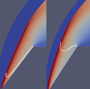
In the computation of three-dimensional flows of this kind a critical aspect is that the boundaries of the subsonic region embedded in the supersonic flow be well resolved. This is particularly important in the region of the ends of the wedge, where the sonic surface has complex features. For this reason, the grid of 1.4 million cells was clustered in all three directions toward the wedge corner. Figure 4 shows an example of the view of the edge of the wedge with the colours highlighting the trace of the sonic surface in the  $y$-normal symmetry plane and in the wedge surface.

Figure 4. View of the  $y$-normal symmetry plane and the inside of the wedge, near the outer edge of the wedge. The flow is from left to right and the colour shows subsonic areas blue, supersonic areas red. The slightly darker blue and red areas are the wedge flank surface. Note how the trace of the sonic surface on the left of the figure first follows the bow shock and then makes a tight curve to the outer corner of the wedge. Note also the trace of the sonic surface in the wedge flank surface. Here,
  $w=51$ mm,
  $\varLambda =3$,
  $\theta =50^\circ$, ideal nitrogen.
The quantity of interest in these computations is the slope  $\textrm {d}\varDelta /\textrm {d}\theta$, or
  $\varDelta _\theta$ near detachment. It was determined by performing two computations at values of
  $\theta$ close to
  $\theta _d$ for each aspect ratio
  $\varLambda =L/w$. In figure 5
  $\varDelta _\theta$, normalized by the value obtained from a two-dimensional computation is plotted against aspect ratio. This also shows that a fair approximation to the results is given by the function
  $\tanh (\varLambda /4.5)$. Also shown in the figure are experimental points from Hornung & Schoeler (Reference Hornung and Schoeler1985). These experimental points were recalculated using only measured points with larger detachment distance because those are considered more accurate. Unfortunately, this was not possible at the smallest of the three aspect ratios, for which the uncertainty is therefore much larger.

Figure 5. Normalized slope  $\textrm {d}\varDelta /\textrm {d}\theta$ at
  $\theta =\theta _d$ as a function of aspect ratio from three-dimensional computations. Open circles: ideal nitrogen flow at
  $M_\infty =5.66$,
  $\gamma =1.4$, open triangles: thermally perfect CO
 $_2$ flow,
  $M_\infty =7.4$, open squares: ideal argon flow at
  $M_\infty =8$,
  $\gamma =5/3$, filled circles: experiments of Hornung & Schoeler (Reference Hornung and Schoeler1985). The blue line is
  $\tanh (\varLambda /4.5)$.
The results enable us to write an analytical form for the detachment distance on a finite wedge as
 \begin{equation} \frac{\varDelta}{w}=\tanh(\varLambda/4.5)\sqrt{\varepsilon}(1+1.5\varepsilon)(2.2\eta-0.3\eta^2)\sin{\theta}. \end{equation}
As always, although approximate, such analytical forms are very powerful tools.
5. Three-dimensional non-equilibrium nitrogen flow
5.1. Nominal free-stream conditions
The free-stream conditions reported in Hornung & Smith (Reference Hornung and Smith1979) were determined by first determining the reservoir conditions from the measured initial shock tube pressure and temperature, the measured shock speed and the measured reservoir pressure, assuming equilibrium processes. The nozzle exit conditions were then found by a one-dimensional non-equilibrium nozzle-flow integration in which vibration was assumed to be in equilibrium. In order to improve on this, the nozzle flow was recomputed with viscous axisymmetric flow and with the same two-temperature reacting gas model as in § 3. The nozzle exit conditions obtained from this computation are shown in figure 6.

Figure 6. Profiles of flow variables across the exit plane of the T3 nozzle as computed from the data of Hornung & Smith (Reference Hornung and Smith1979) in axisymmetric flow with the reaction model of Park (Reference Park1993). Here,  $r$ is the radial coordinate in the nozzle exit plane.
The most important difference between these conditions and those given by Hornung & Smith (Reference Hornung and Smith1979) is that the vibrational temperature is much higher than the translational temperature. Although there are other minor differences between the two, the nominal conditions for our computations are taken to be as given in table 2.
Table 2. Nominal free-stream conditions for the nitrogen computations.
5.2. The effect of the boundary layer
In order to compare computational and experimental results in this case it is important to determine how important the viscous boundary layer is in the shock detachment distance. The resolution requirements for viscous flows are much more stringent than for inviscid flows and it would save substantial computational time if only the inviscid case needed to be computed. In the following we therefore test the effect of the boundary layer in a particular representative case.
To examine this question, a viscous and an inviscid flow were computed with  $\theta =60^\circ$. Figure 7 shows a comparison of the profiles of velocity magnitude
  $q$ and density
  $\rho$ as well as their product
  $\rho q$ plotted against distance normal to the wall
  $n$ at a point 30 mm from the wedge tip in the symmetry plane (
 $w=51$ mm). The distance of the grid point nearest to the wall in these computations was 2.5
  $\mathrm {\mu }$m from the wall, which is of order 1 viscous length. The integral of the difference between the viscous and inviscid values of
  $\rho q$ over
  $n$ is a measure of the displacement effect of the boundary layer. Although the viscous curve for
  $\rho q$ is somewhat noisy near the wall, and an accurate displacement thickness cannot be determined from the data, it is clear from the comparison that the displacement effect is very small.

Figure 7. Profiles of density, velocity magnitude and their product in the boundary layer at 30 mm from the wedge tip in the  $z$-normal symmetry plane. Two-temperature reacting nitrogen,
  $\theta =60^\circ$,
  $\varLambda =3$. The fat lines are for viscous flow and they are compared with thin lines for inviscid flow.
This may be tested further by a comparison of the temperature distributions in the immediate vicinity of the point where the stagnation streamline crosses the shock, see figure 8. It is clear from this figure that the effect of viscosity on  $\varDelta$ is small enough to be ignored, amounting to less than 1 %. We therefore consider that inviscid computations suffice for the comparison with the experiment.

Figure 8. Enlarged views of the temperature distribution in the region where the stagnation streamline crosses the shock wave in the two flows of figure 7. (a) Inviscid flow, (b) viscous flow. The two green lines are rulers measuring the distance from the stagnation point. These are separated in the  $y$-direction by a distance of 30
  $\mathrm {\mu }$m and measure 4.96 and 4.99 mm.
5.3. Computational results and comparison with experiment
As for the non-relaxing flows in § 4, three-dimensional computations were made with the two-temperature reacting flow model used in § 3, for a wedge with  $\varLambda =3$,
  $w=51$ mm, at the free-stream conditions of table 2. The results are shown in figure 9 in comparison with the experiments of Hornung & Smith (Reference Hornung and Smith1979). Also shown in the figure are computations of frozen and equilibrium flow at the same free-stream conditions. The striking feature about the figure is that the computational results, shown as filled squares, are quite precisely displaced to the right from the experiments (faster reaction) by
  $4^\circ$. This is a large discrepancy. It is interesting to note that the reaction rates measured by Hanson & Baganoff (Reference Hanson and Baganoff1972), using pressure measurements in a shock tube, and those measured by Kewley & Hornung (Reference Kewley and Hornung1974), using optical interferometry, agree well with each other and are slower than those of Park (Reference Park1993) in the high-temperature range (10 000–14 000 K) by as much as an order of magnitude. For this reason, additional computations were made with the Kewley & Hornung (Reference Kewley and Hornung1974) rates. The results are shown as filled circles in figure 9. However, as may be seen, the discrepancy is only reduced by a little less than
  $1^\circ$.

Figure 9. Comparison of three-dimensional computations with the experiments of Hornung & Smith (Reference Hornung and Smith1979) (HS),  $w=51$ mm,
  $\varLambda =3$, free stream: nitrogen, as table 2. Open squares: experiment. Filled squares: rates of Park (Reference Park1993), filled circles: rates of Kewley & Hornung (Reference Kewley and Hornung1974) (KH), filled black triangles: frozen flow, filled red triangles: equilibrium flow. The blue line is a smoothed fit to the experimental data. The thin red lines are (4.6) with
  $\varepsilon$ determined from the density ratios at these conditions, in very good agreement with the computations.
At this point it is important to relate this result to earlier experiments on dissociating nitrogen flow over circular cylinders performed in the same facility but with a conical nozzle by Hornung (Reference Hornung1972), in which good agreement with two-dimensional computations was observed, specifically between an experimental and computed interferogram of cylinder flow. Cylinder flows are, of course, much less sensitive to relaxation effects than shock detachment from a wedge. However, both source-flow (conical nozzle) and finite-span effects were shown in Hornung & Smith (Reference Hornung and Smith1979) to have the same effect on detachment distance as a faster reaction. Taking proper account of them in computing the cylinder flows would therefore cause a discrepancy of the same sign to be observed there too.
5.4. Tests of possible causes of the discrepancy
In order to examine possible reasons for the discrepancy between experiment and computation that is evident from figure 9, a number of additional computations were made by changing one parameter at a time.
By deliberately reducing all the reaction rates by a factor of 10, the computed detachment distance is brought into agreement with the experiment, see the filled squares in figure 10. This is a much greater change than is credible, since the uncertainty in the reaction rates is more like a factor of 2.

Figure 10. The effect of changing parameters one at a time on the discrepancy. For reference, the frozen and equilibrium results are repeated as in figure 9. Filled black squares: reactions reduced by a factor of 10. Filled red circles: free-stream speed reduced to 5 km s $^{-1}$. Filled green squares: free-stream atomic nitrogen mass fraction increased to 27 %. Filled blue squares: helium contamination mass fraction set to 3.4 %. HS denotes Hornung & Smith (Reference Hornung and Smith1979).
Next, the free-stream speed was reduced from 5.5 to 5.0 km s $^{-1}$. This yielded the results shown as filled red circles in figure 10. Again this step brings the results into line with the experiment, and again, the change is more than twice the uncertainty in
  $u_\infty$.
Another change was to increase the free-stream atomic nitrogen mass fraction to 27 %, with the results shown as filled green squares in figure 10. This change again brings the results into line with the experiment, but it is much larger than a credible uncertainty.
Finally, a gas model was constructed in which helium was added as a passive component. This was done in order to examine the effect that contamination of the test gas with helium driver gas would have on the measurements. The experiments of Sudani & Hornung (Reference Sudani and Hornung1998) showed that driver-gas contamination occurs in two stages, an early stage in which the concentration of driver gas is limited, followed by a massive increase at a later time. It is possible that the time of the Hornung & Smith (Reference Hornung and Smith1979) experiments occurred during the first stage of contamination. Results obtained with a helium mass fraction of 3.4 % are shown in figure 10 as filled blue squares. This effect reduces the discrepancy by a factor of approximately two.
One might argue that a combination of these four effects, each within a credible limit of uncertainty, could add up to explain the discrepancy. However, we would consider this to be too much of a coincidence. The problem can only be effectively resolved by a repeat of the experiment with more accurately characterized conditions, e.g. using spectroscopic methods such as have recently been applied at Caltech's T5 facility by Girard et al. (Reference Girard, Finch, Strand, Hanson, Yu, Austin and Hornung2021), giving free-stream velocity, temperature and species concentration.
6. Three-dimensional non-equilibrium carbon dioxide flows
The nozzle flow was again recomputed with a two-temperature reacting carbon dioxide model. In this case the vibrational degrees of freedom remained virtually in equilibrium in the nozzle expansion. The free-stream conditions agree well with those given by Hornung & Smith (Reference Hornung and Smith1979) and are given in table 3.
Table 3. Free-stream conditions for the carbon dioxide computations.
In figure 11 the results of three-dimensional computations with this gas model are compared with the carbon dioxide experiments of Hornung & Smith (Reference Hornung and Smith1979). In this case, the computations agree remarkably well with the experiments. However, as may be seen from the figure, the conditions in this carbon dioxide flow are very close to equilibrium, where the sensitivity of the detachment process to non-equilibrium effects disappears. Since driver-gas contamination would move the results to smaller  $\theta$, it appears that there is no evidence of it here.

Figure 11. Comparison of the carbon dioxide experiments with computations. The black and red triangular points again show computed results with frozen and equilibrium flows respectively, and the red curves are (4.6) with  $\varepsilon$ determined from the density ratios at these conditions, again showing very good agreement. HS denotes Hornung & Smith (Reference Hornung and Smith1979); 2T denotes two-temperature.
7. Conclusions
An extensive computational analysis was made of an experiment on the shock detachment process in high-enthalpy non-equilibrium flows of nitrogen and carbon dioxide over a wedge. The sensitivity of this kind of flow to relaxation was demonstrated with two-dimensional non-equilibrium computations. A new extension of an analytical expression for the dimensionless shock detachment distance to three-dimensional flow was found by performing and analysing new three-dimensional computations of non-relaxing flows. New three-dimensional computations of reacting nitrogen and carbon dioxide flows were made and compared with the experiments. In the case of the nitrogen flows a significant discrepancy was observed. Although the trend of the results in the  $\theta$ -
  $\varDelta /w$ plot followed the behaviour exhibited by the experiment, the computational results were displaced from the experiment by 4
 $^\circ$ to larger
  $\theta$, i.e. to faster reaction. Computations in the frozen and equilibrium limits agreed very well with the new analytical expression. Four possible effects that might explain the discrepancy were analysed quantitatively. In each case, the magnitude of the change needed for agreement was much larger than a credible uncertainty. We conclude that, to resolve the discrepancy, the experiment needs to be repeated in more accurately characterized conditions. The comparison in the case of reacting carbon dioxide flow showed very good agreement. However, since the conditions in that case were very close to equilibrium, where the sensitivity of the detachment process is very small, this result is expected.
Declaration of interests
The authors report no conflict of interest.
Appendix. Reaction rate parameters
Table 4. Nitrogen dissociation rates from Kewley & Hornung (Reference Kewley and Hornung1974).

Table 5. Nitrogen dissociation rates from Park (Reference Park1993).

Table 6. Carbon dioxide mixture reaction rates from Ebrahim & Hornung (Reference Ebrahim and Hornung1973).


