1. INTRODUCTION
In general navigation, position is often the only information needed. However, in some special applications, such as vehicle-mounted or airborne mobile mapping systems, in addition to the position, the attitude is needed to control the mapping system's cameras, laser scanners and other sensors (El-Sheimy and Schwarz, Reference El-Sheimy and Schwarz1998; Kukko et al., Reference Kukko, Kaartinen, Hyyppä and Chen2012).
As an Inertial Navigation System (INS) can provide high-sampling rate position and attitude information, it is always selected as the basic navigation system in mobile mapping systems. However, given the influence of gyro drift and accelerometer bias, the navigation errors of the INS gradually accumulate over time. Thus, long-term use will cause large position and attitude errors (Hwang et al., Reference Hwang, Oh, Lee, Park and Rizos2005).
To correct the navigation errors of the INS, other navigation systems are integrated with it, most commonly Global Navigation Satellite Systems (GNSS). Due to the high accuracy and reliability of Differential GNSS (DGNSS), DGNSS/INS integrated navigation has attracted research interest (Redmill et al., Reference Redmill, Kitajima and Ozguner2001; Zhao et al., Reference Zhao, Chen, Zhang and Farrell2014). The inconvenience of DGNSS/INS integrated navigation is that a base station must be built or be available. To ensure the system's accuracy, the mobile system can only work within tens of kilometres of the base station. Therefore, more base stations must be built for wide-range mobile mapping, which increases the complexity and the cost of the work (Liu et al., Reference Liu, Sun, Zhang, Li and Zhu2015).
In recent years, Precise Point Positioning (PPP) technology has undergone rapid development, and dynamic positioning accuracy has improved greatly (Kouba and Héroux, Reference Kouba and Héroux2001). To overcome the restriction imposed by the base station in mobile mapping systems, PPP/INS integrated navigation has been investigated (Du and Gao, Reference Du and Gao2010; Liu et al., Reference Liu, Sun, Zhang, Li and Zhu2015, Rabbou and El-Rabbany, Reference Rabbou and El-Rabbany2014). The results show that ambiguity-fixed PPP/INS integrated navigation can achieve position accuracy similar to that of DGNSS/INS (Liu et al., Reference Liu, Sun, Zhang, Li and Zhu2015). However, it is also found that when a low-accuracy INS is used, obvious attitude errors arise in the PPP/INS solution. In particular, when the vehicle is stationary or maintains uniform motion in one direction, the attitude errors increase significantly. Therefore, the attitude accuracy of PPP/INS does not meet the requirements of mobile mapping systems. A high-accuracy INS would ensure a highly accurate attitude, but they are often too expensive for civil systems. Hence, it is necessary to research other methods to improve attitude accuracy.
To solve this problem, the velocity heading of single-antenna GNSS has been used to provide yaw constraints for the INS (Lai and Jan, Reference Lai and Jan2011; Li et al., Reference Li, Efatmaneshnik and Dempster2012, Tenn et al., Reference Tenn, Jan and Hsiao2009), and this is a simple and convenient method. However, when the vehicle's speed is low, the velocity heading is noisy, and when the vehicle changes direction, the errors in the velocity heading increase.
The integration of double-antenna GNSS and INS has been researched, combining the yaw angle calculated from a single GNSS baseline and the pitch and roll angles calculated from the acceleration measurements with INS attitude to improve attitude accuracy (Wu et al., Reference Wu, Yao, Ma and Jia2013). Although this method improves the accuracy of the yaw angle, it is not very effective for pitch and roll angles. The pitch and roll angles are calculated on the assumption that the vehicle is moving with constant speed. When the vehicle is maneuvering, the accuracies of the pitch and roll angles will decrease, and aided methods are needed. In addition, the vibration of the vehicle adds large amounts of noise to the acceleration measurements, and the noise propagates to the pitch and roll angles.
Airborne Multi-Antenna GNSS (MAGNSS)/INS integrated navigation has also been investigated, making use of attitude measured by MAGNSS to correct the errors of INS attitude and improve the estimated attitude accuracy (Hwang et al., Reference Hwang, Oh, Lee, Park and Rizos2005). Due to the different observation conditions, the algorithms of MAGNSS/INS integrated navigation need to be redesigned for land vehicles. In addition, the attitude errors of an INS increase with time, and the attitude errors of the PPP/INS integration are related to the dynamic status of the vehicle due to poor observability. For evaluating the attitude errors, long-term datasets are best suited. With too short a measurement timespan it is difficult to investigate the differences between the attitude errors of PPP/INS and MAGNSS/INS integration.
In this paper, a MAGNSS/INS integrated navigation system without a base station is designed to provide high-accuracy position and attitude information for vehicle-mounted mobile mapping systems. Owing to the length restrictions of MAGNSS baselines for a normal-size vehicle and the fact that GNSS signals are easily influenced by trees and buildings, it is more difficult to implement MAGNSS/INS integrated navigation on land vehicles than on aircraft. Therefore, a reasonable initial alignment and navigation algorithm is developed, which simultaneously makes use of the PPP position, PPP velocity, and MAGNSS attitude as measurements in a Kalman filter to correct for INS errors.
To test the reliability and accuracy of the position and attitude of the MAGNSS/INS integrated navigation system, a tactical-grade INS was used for a vehicle test which lasted for three hours. The attitude and position solutions from the integration of the DGNSS and the navigation-grade INS were used as references. The attitude solutions of the MAGNSS, PPP/INS and MAGNSS/INS integration and the position solutions of the PPP/INS and MAGNSS/INS integration were evaluated. Detailed analyses of the experimental data were performed.
2. MAGNSS ATTITUDE DETERMINATION
Using differential carrier-phase measurements from MAGNSS mounted on a vehicle, the baseline vectors among the antennae can be calculated precisely and then the attitude of the vehicle can be determined from these baseline vectors (Aleshechkin, Reference Aleshechkin2011; Li and Murata, Reference Li and Murata2002; Lu, Reference Lu1995; Shuster and Oh, Reference Shuster and Oh1981). At least three antennae are needed to determine all three attitude angles of the vehicle simultaneously. In this paper, an attitude-determination method using three-antenna GNSS is introduced.
The antennae are mounted on the roof of the vehicle, and Antenna 1 is set as the main antenna. The baseline between Antenna 1 and Antenna 2 is parallel to the vehicle's longitudinal axis. A right-handed coordinate system is built, as shown in Figure 1. Under the condition of causing no mixes, this coordinate system is set as body frame O−X bY bZ b. The relationship between the Earth frame, navigation frame and body frame is illustrated in Figure 2. The coordinates of Antenna 1, Antenna 2 and Antenna 3 in the body frame are (0, 0, 0), (0, L 12, 0) and (L 13sinθ, L 13cosθ, 0). L 12 is the distance between Antenna 1 and Antenna 2, and L 13 is the distance between Antenna 1 and Antenna 3.
Figure 1. Attitude determination using three-antenna GNSS.
Figure 2. The relationship between the Earth frame, navigation frame and body frame.
At each epoch, the coordinates of Antenna 1 in WGS84 can be obtained from PPP, and the baseline vectors of Antenna 1 to Antenna 2 and Antenna 3 in WGS84 can be determined from differential carrier-phase observations. s12,e and s13,e are used to denote the two baseline vectors:
 $${{\bi s}}_{12,e}=\left[\matrix{x_{12,e} \cr y_{12,e} \cr Z_{12,e}} \right]=\left[\matrix{x_{2,e} & -x_{1,e} \cr y_{2,e} & -y_{1,e} \cr Z_{2,e} & -z_{1,e}} \right]$$
 $${{\bi s}}_{13,e}=\left[\matrix{x_{13,e} \cr y_{13,e} \cr Z_{13,e}} \right]=\left[\matrix{x_{3,e} & -x_{1,e} \cr y_{3,e} & -y_{1,e} \cr Z_{3,e} & -z_{1,e}} \right]$$
In the navigation frame, they are expressed as:
 $${{\bi s}}_{12,n}=\left[\matrix{x_{12,n} \cr y_{12,n} \cr Z_{12,n}} \right]={{\bi C}}_{e}^{n}{{\bi s}}_{12,e}$$
 $${{\bi s}}_{13,n}=\left[\matrix{x_{13,n} \cr y_{13,n} \cr Z_{13,n}} \right]={{\bi C}}_{e}^{n}{{\bi s}}_{13,e}$$
 ${{\bi C}}^{n}_{e}$ can be calculated from the WGS84 coordinates of Antenna 1:
 $${{\bi C}}_{e}^{n}=\left[\matrix{-\sin\lambda & \cos\lambda & 0 \cr -\cos\lambda \sin\varPhi & -\sin\lambda \sin\varPhi & \cos\varPhi \cr \cos\lambda \cos\varPhi & \sin\lambda \cos \varPhi & \sin\varPhi} \right]$$
where λ and  $\varPhi$ are the longitude and latitude of Antenna 1, which are obtained from PPP.
From Figure 1, we can see that the coordinates of the two baselines in the body frame are:
 $${{\bi s}}_{12,b}=\left[\matrix{0 \cr L_{12} \cr 0} \right]$$
 $${{\bi s}}_{13,b}=\left[\matrix{L_{13}\sin\theta \cr L_{13}\cos\theta \cr 0} \right]$$
The relationship of the coordinates of the baseline between Antenna 1 and Antenna 2 in the body frame and navigation frame is:
 $${{\bi s}}_{12,n}=({{\bi C}}_{n}^{b})_{{{\bi s}}_{12,b}}^{T}$$
 ${{\bi C}}^{b}_{n}$ in Equation (8) denotes the attitude matrix, which is used to transform coordinates from the navigation frame to the body frame. It can be transformed using the Euler angles:
 $$\eqalign{C_{n}^{b}&=R_{2}(\alpha)R_{1}(\beta)R_{3}(-\gamma) \cr &=\left[\matrix{\cos\alpha & 0 & -\sin\alpha \cr 0 & 1 & 0 \cr \sin\alpha & 0 & \cos\alpha} \right]\left[\matrix{1 & 0 & 0 \cr 0 & \cos\beta & \sin\beta \cr 0 & -\sin\beta & \cos\beta} \right]\left[\matrix{\cos\gamma & -\hbox{s}\dot{\hbox{m}}\gamma & 0 \cr \sin\gamma & \cos\gamma & 0 \cr 0 & 0 & 1} \right] \cr &=\left[\matrix{\cos\alpha \cos\gamma+\sin\alpha \sin\beta \sin\gamma & -\cos\alpha \sin\gamma+\sin\alpha \sin\beta \cos\gamma & -\sin\alpha \cos\beta \cr \cos\beta \sin\gamma & \cos\beta \cos\gamma & \sin\beta \cr \sin\alpha \cos\gamma-\cos\alpha \sin\beta \sin\gamma & -\sin\alpha \sin\gamma-\cos\alpha \sin\beta \cos\gamma & \cos\alpha \cos\beta} \right]}$$
These Euler angles are also called attitude angles, where α denotes the roll angle; β denotes the pitch angle; γ denotes the yaw angle and clockwise is positive. They are illustrated in Figure 2.
Substituting Equations (3), (6) and (9) into Equation (8):
 $$\left[\matrix{x_{12,n} \cr y_{12,n} \cr Z_{12,n}} \right]=\left[\matrix{\cos\beta & \sin\gamma \cr \cos\beta & \cos\gamma \cr \sin\beta &} \right]L_{12}$$
From Equation (10), the yaw angle is:
 $$\gamma=\arctan \left(\displaystyle{x_{12,n} \over y_{12,n}}\right) $$
The pitch angle is:
 $$\beta=\arctan\left(\displaystyle{Z_{12,n} \over \sqrt{x_{12n}^{2}+y_{12,n}^{2}}}\right)$$
The relationship of the coordinates of the baseline between Antenna 1 and Antenna 3 in the body frame and navigation frame is:
 $${{\bi s}}_{13,b}={{\bi C}}_{n}^{b}{{\bi s}}_{13,n}$$
Substituting Equations (4), (7) and (9) into Equation (13):
 $$\eqalign{&\left[\matrix{L_{13}\sin\theta \cr L_{13}\cos\theta \cr 0} \right]={{\bi R}}_{2}(\alpha){{\bi R}}_{1}(\beta){{\bi R}}_{3}(-\gamma)\left[\matrix{x_{13,n} \cr y_{13,n} \cr Z_{13,n}} \right] \cr &\quad=\left[\matrix{\cos\alpha & 0 & -\sin\alpha \cr 0 & 1 & 0 \cr \sin\alpha & 0 & \cos\alpha} \right] \left[\matrix{x_{13,n} \cos\gamma-y_{13,n}\sin\gamma \cr x_{13,n}\cos\beta \sin\gamma+y_{13,n} \cos\beta \cos\gamma+z_{13,n} \sin\beta \cr -X_{13,n}\sin\beta \sin\gamma-y_{13,n} \sin\beta \cos\gamma+z_{13,n} \cos\beta} \right]}$$
From Equation (14), the roll angle is:
 $$a=-\arctan \left(\displaystyle{-x_{13,n}\sin\beta\sin\gamma-y_{13,n}\sin\beta\cos\gamma+z_{13,n}\cos\beta \over x_{13,n}\cos\gamma-y_{13,n}\sin\gamma}\right) $$
From Equations (11), (12) and (15), the attitude can be determined using only the coordinates of the baseline vectors in the navigation frame, and the coordinates in the body frame are unnecessary. However, this method is only applied when three antennae are used; if more antennae are mounted, the least squares method is needed.
3. MAGNSS/INS INTEGRATED NAVIGATION
3.1. INS navigation algorithm
The vehicle's attitude, velocity and position can be determined by integrating the acceleration and angular rate sensed by the INS. Generally, Strapdown INS (SINS) is used, which measures the acceleration and angular rate in the body frame. The relationship of the acceleration and angular rate with the attitude, velocity and position can be expressed by the navigation equation. In the navigation frame, the navigation equations are:
 $$\dot{{{\bi C}}}_{b}^{n} ={{\bi C}}_{b}^{n}({\bf \omega}_{nb}^{b}\times)$$
 $$\dot{{{\bi v}}}^{n} ={{\bi f}}^{n}-(2{\bf \omega}_{ie}^{n}+{\bf \omega}_{en}^{n})\times {{\bi v}}^{n}+{{\bi g}}^{n}$$
 $$\dot{\varPhi} =\displaystyle{v_{N} \over R_{M}+h} \dot{\lambda}=\displaystyle{v_{E}\sec\varPhi \over R_{N}+h} \dot{h}=v_{U}$$
 Equation (16) is the attitude differential equation, where  ${{\bi C}}^{n}_{b}$ is the attitude matrix, and
  ${\bf \omega}^{b}_{nb}$ is the angular rate vector of the body frame with respect to the navigation frame resolved in the body frame. To avoid the singularity problem, the attitude can be computed by the quaternion update method, and the quaternion can be updated by a rotation vector (Qin, Reference Qin2006; Savage, Reference Savage1998a; Reference Savage1998b).
Equation (17) is the velocity differential equation, where vn is the velocity vector, fn is the specific force vector in the navigation frame,  ${\bf \omega}^{n}_{ie}$ is the angular rate vector of the Earth frame with respect to the inertial frame resolved in the navigation frame,
  ${\bf \omega}^{n}_{en}$ is the angular rate vector of the navigation frame with respect to the Earth frame resolved in the navigation frame and gn is the gravity vector in the navigation frame. To improve the accuracy of the velocity, compensation of rotation and the sculling effect is needed (Qin, Reference Qin2006; Savage, Reference Savage1998a; Reference Savage1998b).
Equation (18) is the position differential equation, where  $\varPhi$ is the latitude; λ is the longitude; h is the height; vE, vN and vU are the tri-axial velocities in the navigation frame; R M is the radius of curvature of the meridian and R N is the radius of curvature of the prime vertical. Here, Equation (18) describes a simplified method that neglects the compensation of rotation and scrolling effects but is still sufficiently accurate.
3.2. MAGNSS/INS integration
Due to the errors of gyros and accelerometers, the navigation solution from INS mechanisation may drift with time, and the drift rate depends on the accuracies of the gyros and accelerometers. To obtain a long-term stable solution, an external aiding system, such as GNSS, is needed to estimate the navigation errors. The error equations of the INS are expressed as the differential equations of the misalignment angle ψ, velocity error δ v and position error δ p. The tri-axial error equations are (Qin, Reference Qin2006):
 $$\eqalign{\dot{\psi}_{E}&=\psi_{N}\left(\omega_{ie}\sin\varPhi+\displaystyle{v_{E} \over R_{N}+h}\tan\varPhi \right) -\psi_{U} \left(\omega_{ie}\cos\varPhi+\displaystyle{v_{E} \over R_{N}+h}\right) \cr &\quad -\displaystyle{\delta v_{N} \over R_{M}+h}+\delta h\displaystyle{v_{N} \over (R_{M}+h)^{2}}-\varepsilon_{E}}$$
 $$\eqalign{\dot{\psi}_{N}&=-\psi_{E}\left( \omega_{ie}\sin\varPhi+\displaystyle{v_{E} \over R_{N}+h}\tan\varPhi\right) -\psi_{U}\displaystyle{v_{N} \over R_{M}+h}-\delta\varPhi\omega_{ie}\sin\varPhi \cr &\quad +\displaystyle{\delta v_{E} \over R_{N}+h}-\delta h\displaystyle{v_{E} \over (R_{N}+h)^{2}}-\varepsilon_{N}}$$
 $$\eqalign{\dot{\psi}_{U}&=\psi_{E}\left(\omega_{ie}\cos\varPhi+\displaystyle{v_{E} \over R_{N}+h}\right) +\psi_{N}\displaystyle{v_{N} \over R_{M}+h}+\delta\varPhi \left(\omega_{ie}\cos\varPhi+\displaystyle{v_{E} \over R_{N}+h}\sec^{2}\varPhi\right) \cr &\quad +\displaystyle{\delta v_{E} \over R_{N}+h}\tan\varPhi-\delta h\displaystyle{v_{E}\tan\varPhi \over (R_{N}+h)^{2}}-\varepsilon_{U}}$$
 $$\eqalign{\delta \dot{v}_{E}&=\psi_{U}f_{N}-\psi_{N}f_{U}+\delta v_{E}\displaystyle{v_{N}\tan\varPhi-v_{U} \over R_{N}+h}+\delta v_{N} \left(2\omega_{ie}\sin\varPhi+\displaystyle{v_{E} \over R_{N}+h}\tan\varPhi\right) \cr &\quad -\delta v_{U} \left(2\omega_{ie}\cos\varPhi+\displaystyle{v_{E} \over R_{N}+h}\right) +\delta\varPhi\left[ 2\omega_{ie}(v_{U}\sin\varPhi+v_{N}\cos\varPhi)+\displaystyle{v_{E}v_{N} \over R_{N}+h}\sec^{2}\varPhi \right] \cr &\quad +\delta h\displaystyle{v_{E}v_{U}-v_{E}v_{N}\tan\varPhi \over (R_{N}+h)^{2}}+\nabla_{E}}$$
 $$\eqalign{\delta \dot{v}_{N}&=-\psi_{U}f_{E}+\psi_{E}f_{U}-2 \left(\omega_{ie}\sin\varPhi+\displaystyle{v_{E} \over R_{N}+h}\tan\varPhi\right) \delta v_{E}-\delta v_{N}\displaystyle{v_{U} \over R_{M}+h} -\delta v_{U}\displaystyle{v_{N} \over R_{M}+h} \cr &\quad -\delta\varPhi\left( 2v_{E}\omega_{ie}\cos\varPhi+\displaystyle{v_{E}^{2} \over R_{N}+h}\sec^{2}\varPhi\right) +\delta h\left[\displaystyle{v_{N}v_{U} \over (R_{M}+h)^{2}}+\displaystyle{v_{E}^{2}\tan\varPhi \over (R_{N}+h)^{2}}\right] +\nabla_{N}}$$
 $$\eqalign{\delta \dot{v}_{U}&=\psi_{N}f_{E}-\psi_{E}f_{N}+2 \left(\omega_{ie}\cos\varPhi+\displaystyle{v_{E} \over R_{N}+h}\right) \delta v_{E}+\delta v_{N}\displaystyle{2v_{N} \over R_{M}+h}-2\delta\varPhi v_{E}\omega_{ie}\sin\varPhi \cr &\quad -\delta h\left[ \displaystyle{v_{N}^{2} \over (R_{M}+h)^{2}}+\displaystyle{v_{E}^{2} \over (R_{N}+h)^{2}}\right] +\nabla_{U}}$$
 $$\delta\dot{\varPhi} =\displaystyle{\delta v_{N} \over R_{M}+h}-\delta h\displaystyle{v_{N} \over (R_{M}+h)^{2}}$$
 $$\delta\dot{\lambda} =\displaystyle{\delta v_{E} \over R_{N}+h}\sec\varPhi+\delta\varPhi\displaystyle{v_{E} \over R_{N}+h}\tan\varPhi\sec\varPhi-\delta h\displaystyle{v_{E}\sec\varPhi \over (R_{N}+h)^{2}}$$
 $$\delta\dot{h} = \delta v_{U}$$
where ωie is the rotation rate of the Earth; εE, εN and εU are the gyro drifts and ∇E, ∇N and ∇U are the accelerometer biases.
Due to its high efficiency and good performance in practice, the Kalman filter is the most popular method in integrated navigation. The Kalman filter is a type of minimum-variance estimation that uses the state-space method to estimate the state vector in the time domain recursively. Two types of algorithms are used for the Kalman filter: the continuous algorithm and the discrete algorithm. The misalignment angles, velocity errors, position errors, gyro drifts and accelerometer biases are set as the state vector:
 $${{\bi x}}=(\psi_E\ \psi_N\ \psi_U\ \delta \nu_E\ \delta \nu_N\ \delta \nu_U\ \delta\varPhi\ \delta\lambda\ \delta h\ \varepsilon_E\ \varepsilon_N\ \varepsilon_U\ \nabla_E\ \nabla_N\ \nabla_U)$$
The state equation is:
 $$\dot{{{\bi x}}}={{\bi Fx}}+{{\bi W}}$$
The state matrix F can be obtained from Equations (19) to (27). As Equation (29) is a continuous differential equation, it must be discretised before designing the algorithm. W is the system noise, and its variance depends on the noise level of the INS.
The measurement equation is described by:
 $${{\bi z}}={{\bi Hx}}+{{\bi V}}$$
The measurement vector is:
 $${{\bi z}}=\left[\matrix{{\bf \psi}_m \cr \delta {\bf \nu}_m \cr \delta {{\bi p}}_m} \right]$$
where ψm is the measurement of the misalignment angle, which corresponds to the misalignment matrix Cψ. The misalignment matrix Cψ can be calculated by:
 $${{\bi C}}_\psi={{\bi C}}_s({{\bi C}}_b^n)_{GNSS}({{\bi C}}_b^n)_{INS}^T$$
 where CS denotes the systematic attitude offsets between the MAGNSS and the INS,  $({{\bi C}}^{n}_{b})_{INS}$ is the attitude matrix from INS mechanisation,
  $({{\bi C}}^{n}_{b})_{GNSS}$ is the attitude matrix determined from MAGNSS and T denotes the transposition of the matrix.
δ vm in the measurement vector is the difference of the velocities from INS mechanisation and PPP:
 $$\delta {\bf \nu}_m={\bf \nu}_{INS}+{{\bi C}}^n_b({\bf \omega}^b_{eb}\times {{\bi l}}^b)-{\bf \nu}_{GNSS}$$
where lb is the lever arm between the INS and Antenna 1, measured in the body frame,  ${\bf \omega}^{b}_{eb}$ is the angular rate vector of the body frame with respect to the Earth frame resolved in the body frame and
  ${{\bi C}}^{n}_{b}({\bf \omega}^{b}_{eb}\times {{\bi l}}^{b})$ denotes the velocity correction generated by the lever arm.
δ pm in the measurement vector is the difference of the positions from INS mechanisation and PPP:
 $$\delta {{\bi p}}_m={{\bi p}}_{INS}+{{\bi M}}_p{{\bi C}}^n_b{{\bi l}}^b-{{\bi p}}_{GNSS}$$
 where p is the position,  ${{\bi M}}_{p}{{\bi C}}^{n}_{b}{{\bi l}}^{b}$ is the position correction due to the lever arm, and:
 $${{\bi M}}_p=\left[\matrix{0&\displaystyle{1 \over R_M+h} & 0 \cr \displaystyle{\hbox{sec}\,\varPhi \over R_N+h}&0&0 \cr 0&0&1} \right]$$
The measurement matrix H in measurement Equation (30) is:
 $${{\bi H}}=\left[\matrix{{{\bi I}}_{3\times 3} & {{\bi 0}}_{3\times 3} & {{\bi 0}}_{3\times 3} & {{\bi 0}}_{3\times 6} \cr {{\bi 0}}_{3\times 3} & {{\bi I}}_{3\times 3} & {{\bi 0}}_{3\times 3} & {{\bi 0}}_{3\times 6} \cr {{\bi 0}}_{3\times 3} & {{\bi 0}}_{3\times 3} & {{\bi I}}_{3\times 3} & {{\bi 0}}_{3\times 6}} \right]$$
The V in measurement Equation (30) is the measurement noise, and its variance is determined by the accuracies of the position, velocity and attitude from PPP and MAGNSS.
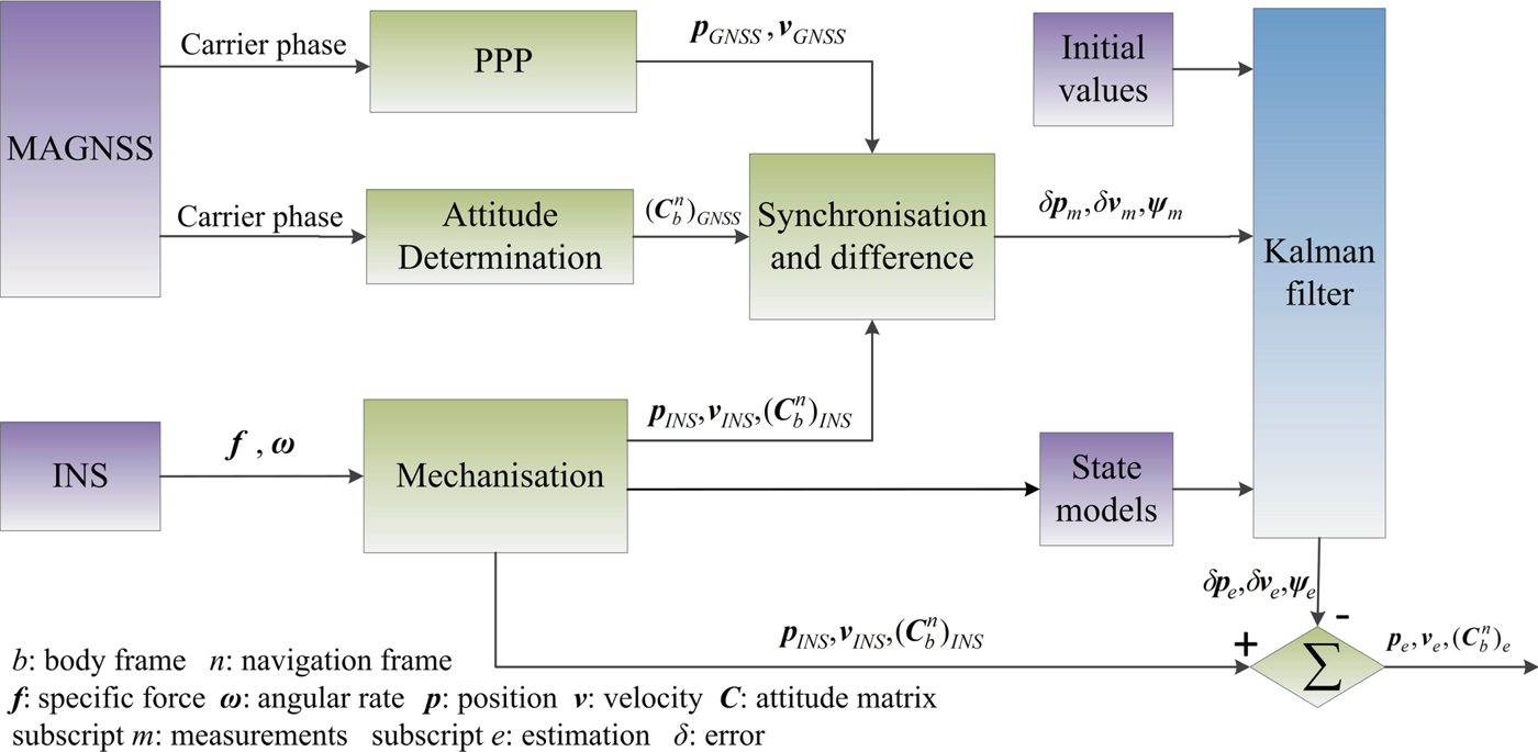
The flow chart of the MAGNSS/INS integrated navigation is shown in Figure 3.

Figure 3. Flow chart of MAGNSS/INS integrated navigation.
4. TEST AND RESULTS
A test was conducted on 28 December 2015 in Wuhan, China to evaluate MAGNSS/INS integrated navigation. A tactical-grade INS and four GNSS receivers were used. The DGNSS/INS solutions from a navigation-grade INS and DGNSS were used as references. The raw specific force increments and angle increments were logged from the INSs at 200 Hz. The raw dual-frequency phase and Doppler observations were logged from the GNSS receivers at 1 Hz. The installation of the GNSS antennae is shown in Figure 4. The test lasted approximately 3 hours, and the vehicle travelled at a speed of approximately 30 to 40 km/h. The horizontal routing and the location of the base station are shown in Figure 5. The vehicle was driven from starting point A past point B to terminal point C and then back to A. Trimble NetR9 receivers were used in the test. The kinematic differential positioning accuracies of the receivers are 8 mm + 0.5 ppm (horizontal) and 15 mm + 0.5 ppm (vertical). The specifications of the INSs are listed in Table 1.

Figure 4. Installation of the GNSS Antennae.
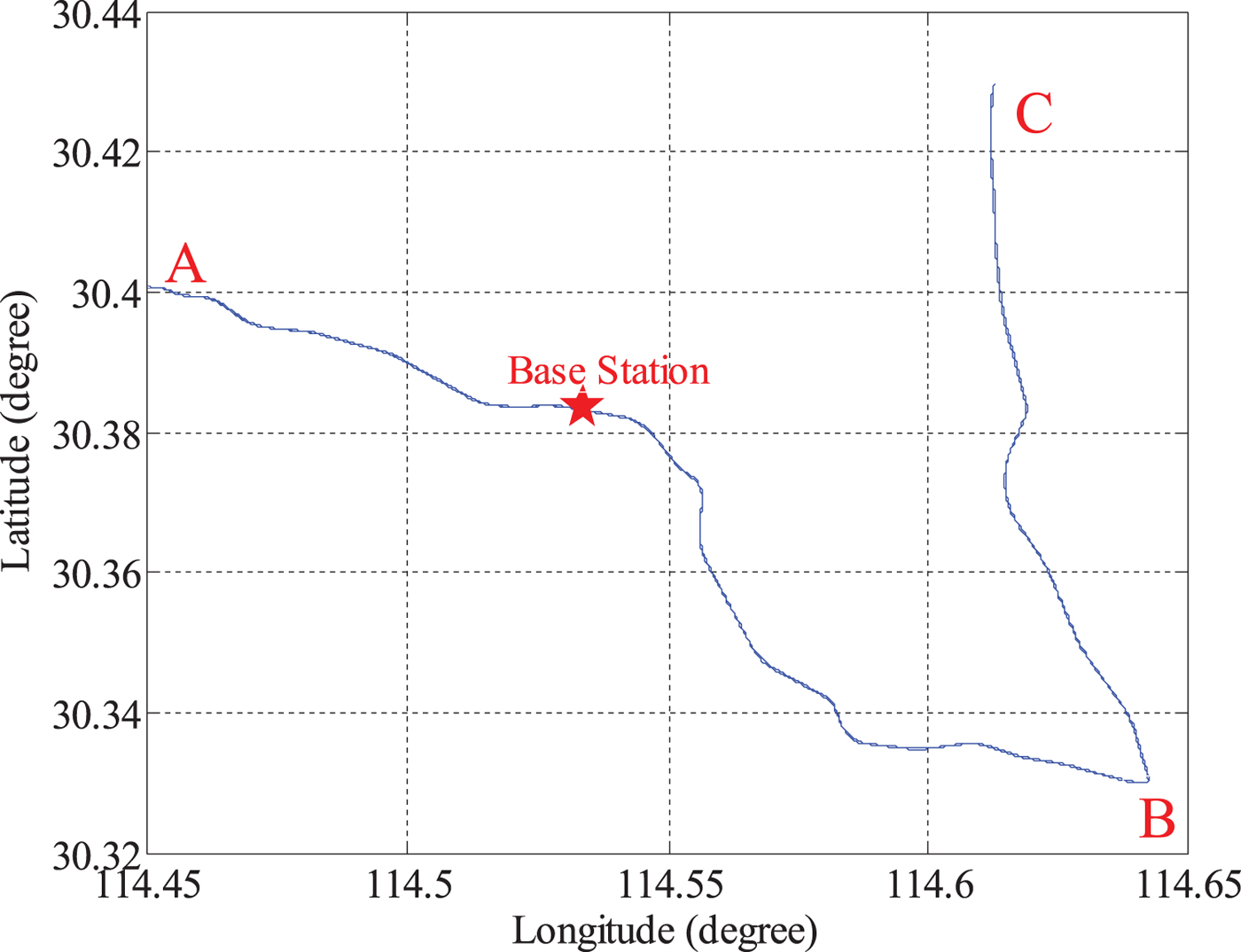
Figure 5. Horizontal routing of the test.
Table 1. Specifications of the Two INSs.
4.1. MAGNSS attitude determination
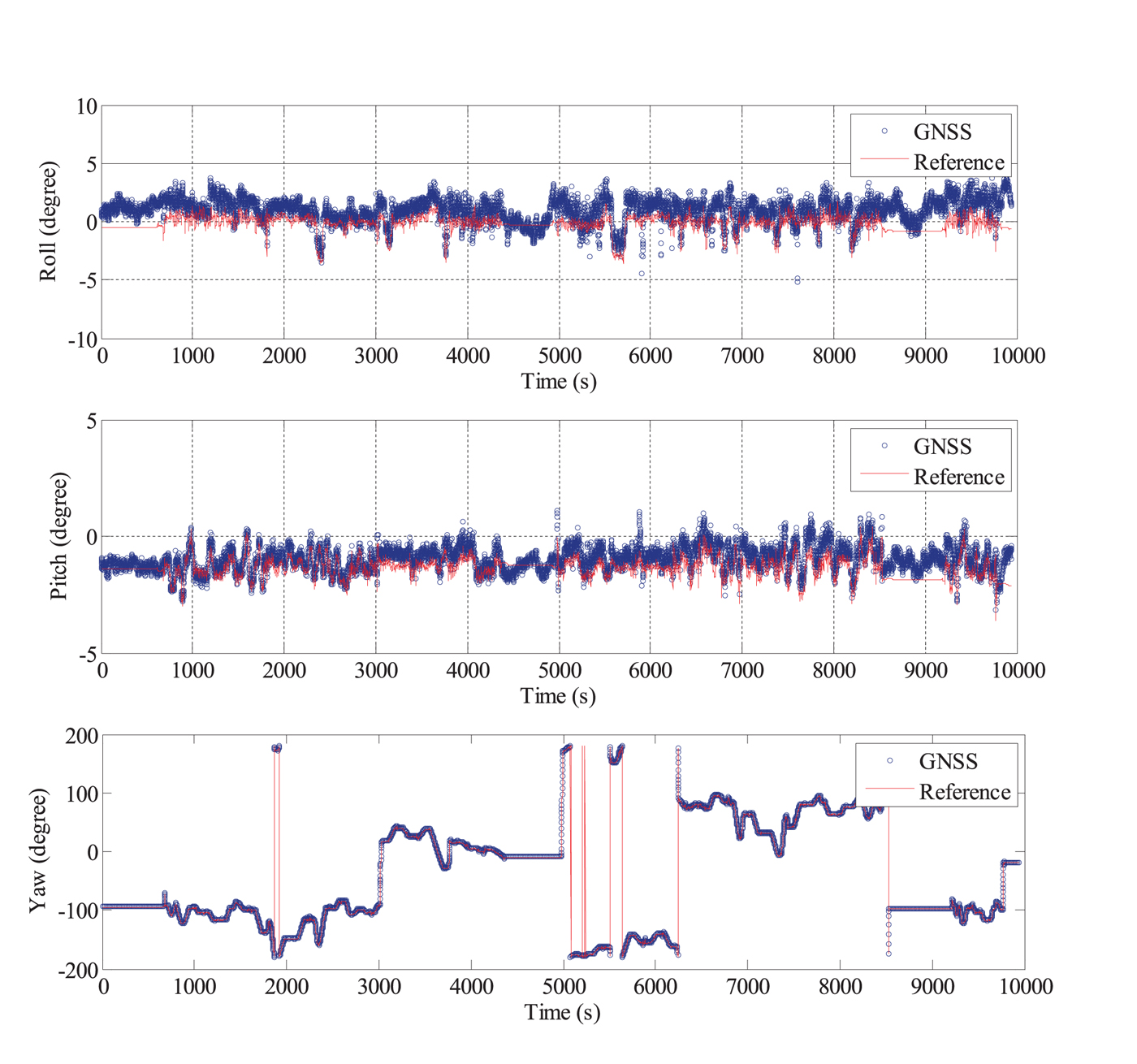
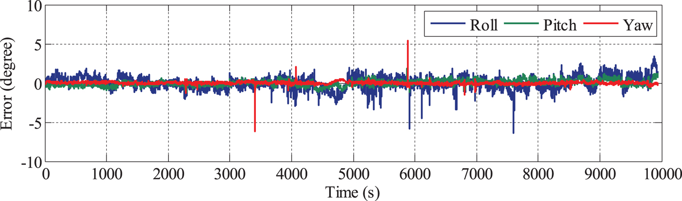
In the data processing, Global Positioning System (GPS) signals and Global Navigation Satellite System (GLONASS) signals were used. The data from Antenna 4 was incomplete and of poor quality due to a problem with a data wire, and thus, the carrier phase measurements from Antenna 1, Antenna 2 and Antenna 3 were used for the calculation of the dynamic baseline vectors s12,e and s13,e. The PPP solutions derived from the carrier phase and Doppler measurements from Antenna 1 were used for the calculation of  ${{\bi C}}^{n}_{e}$. Then, the attitude was derived using the method given in Section 2. The MAGNSS attitude and the reference value are shown in Figure 6. The MAGNSS attitude coincides well with the reference. Some systematic offsets arise between the MAGNSS attitude and the reference because of the misalignment of the MAGNSS and the INS. After removing these offsets, the errors in the MAGNSS attitude are as shown in Figure 7. As shown in Table 2, the standard deviations of the MAGNSS attitude are 0.803° in roll angle, 0.343° in pitch angle and 0.204° in yaw angle.

Figure 6. Comparison of the MAGNSS attitude and the reference value.

Figure 7. MAGNSS attitude error.
Table 2. Statistics of the MAGNSS Attitude Error.

4.2. MAGNSS attitude-aided INS alignment
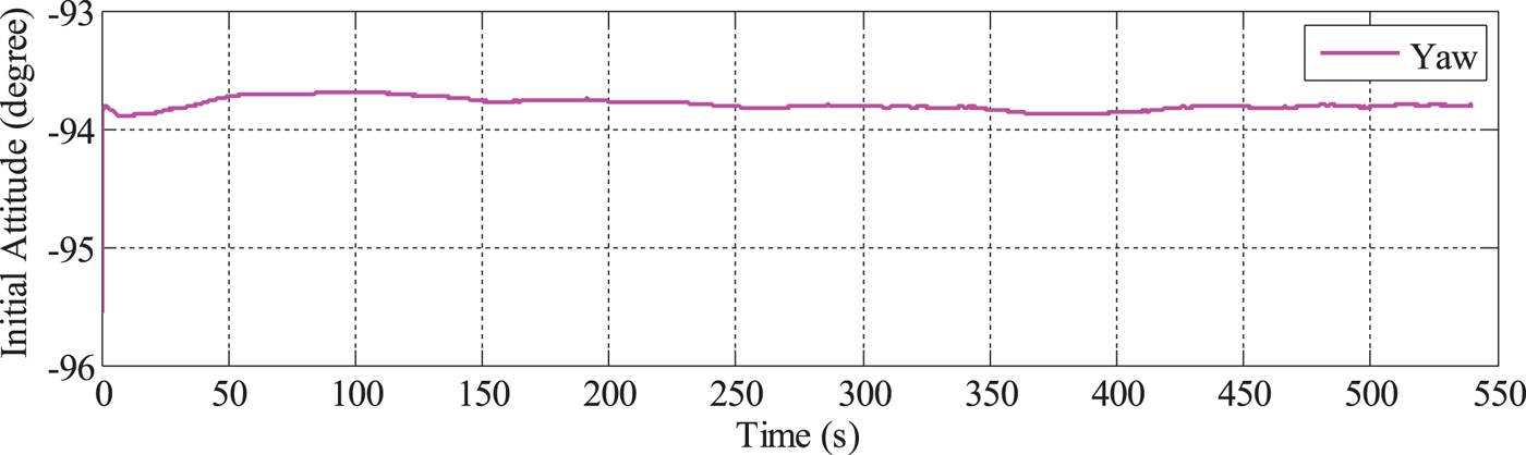
The error of the initial alignment of the low-accuracy INS is largely attributable to the low-grade sensors. Take the tactical-grade INS used in the test for example. The alignment, which lasted 540 s, is illustrated in Figure 8. The roll angle and pitch angle converge quickly, but the yaw angle cannot converge; instead, it fluctuates between −95° and −98°.
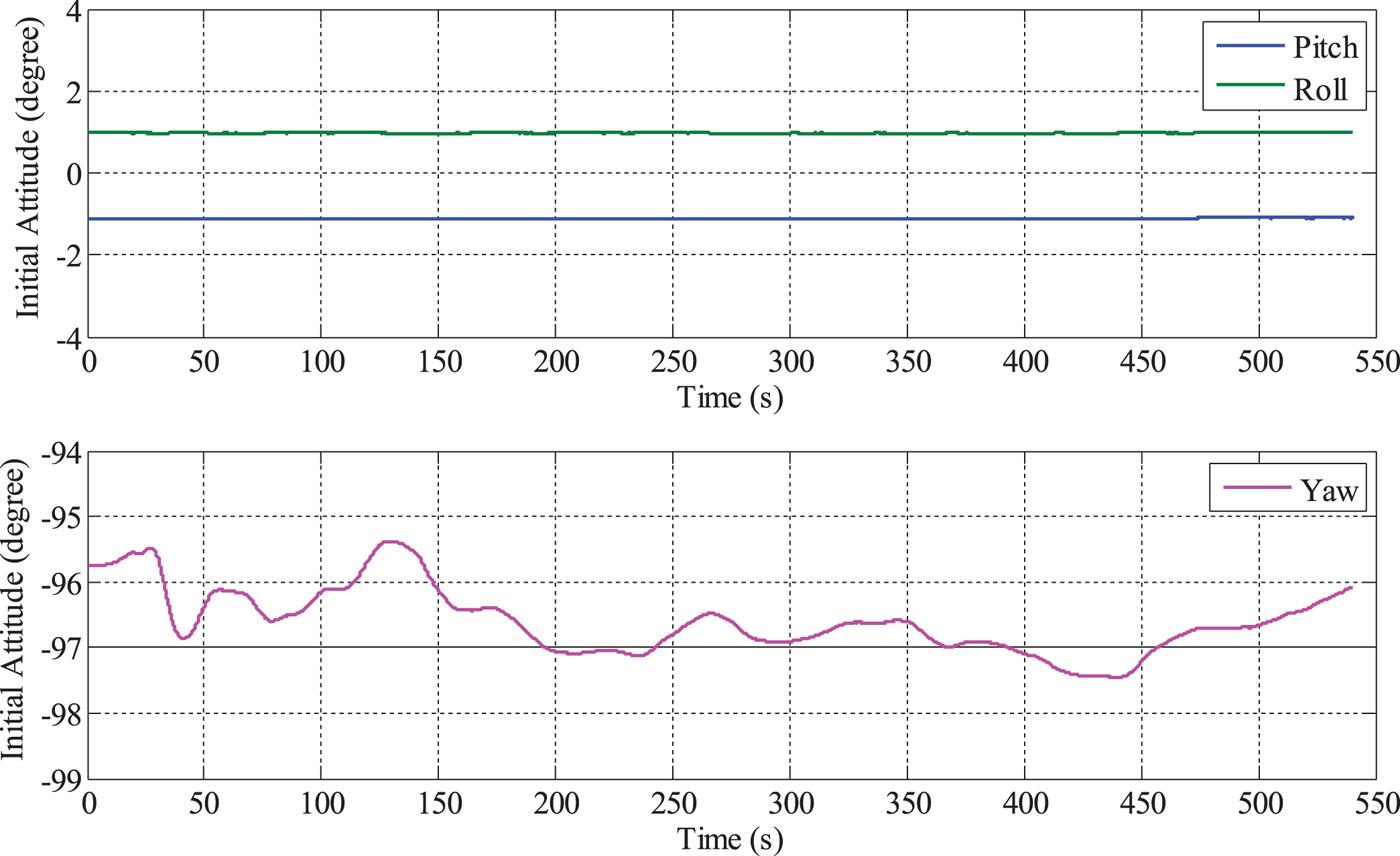
Figure 8. Alignment of the tactical-grade INS.
The initial attitude is the initial datum of INS mechanisation, and thus, the alignment error propagates to the INS mechanisation. In integrated navigation, when GNSS signals are of poor quality, the attitude solution depends more on the INS. To improve the attitude accuracy, the alignment accuracy must also be improved. To achieve this goal, MAGNSS attitude-aided alignment is proposed. As the roll and pitch angle can converge perfectly, in this paper, the alignment is only aided by the MAGNSS yaw angle. The improved yaw angle during the alignment is shown in Figure 9. When aided by the MAGNSS attitude, the yaw angle converges faster and with more accuracy.

Figure 9. Yaw angle during alignment aided by MAGNSS attitude.
4.3. MAGNSS/INS integrated navigation
The PPP solutions derived from the carrier phase and Doppler measurements from Antenna 1 were used for the PPP/INS integration. The attitude solutions of PPP/INS are compared with the reference, and the errors are depicted in Figure 10. It can be seen that the roll and pitch angle are accurate. However, the yaw error is much larger because of its poor observability. In the first 10 minutes, the yaw angle cannot converge because the vehicle does not move, but once the vehicle begins moving, the yaw angle converges. From 112,600 s to 116,150 s, the vehicle travelled in a south-east direction from point A to point B and north from point B to point C. During this period, the yaw errors were less than 0.5°. From 116,800 s to 118,750 s, the vehicle travelled south from point C to point B. During this period, the yaw errors were the largest, ranging from −0.4° to 0.9°. From 118,750 s to 120,180 s, the vehicle travelled north-west from point B to point A, and the yaw errors were less than 0.2°. From 116,150 s to 116,780 s and from 120,300 s to 121,000 s, the yaw errors remained constant because the vehicle did not move.
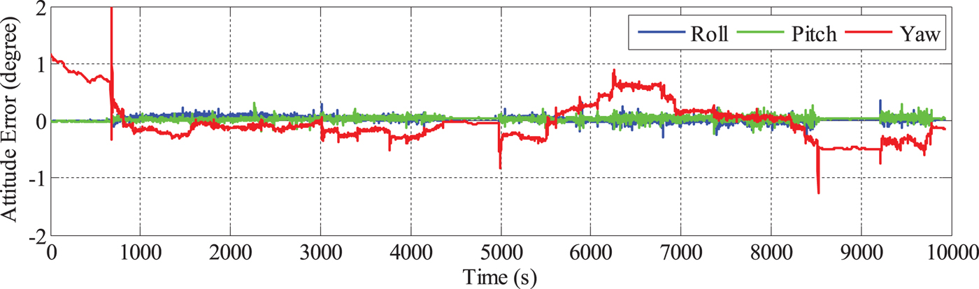
Figure 10. Attitude errors of PPP/INS integrated navigation.
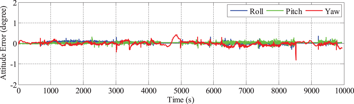
To improve the attitude accuracy of the PPP/INS, the solutions of the proposed MAGNSS/INS integrated navigation are calculated. The systematic errors between the MAGNSS attitude and the INS attitude must be removed. The attitude errors of the MAGNSS/INS solutions are shown in Figure 11. From Figure 11, it can be seen that the yaw accuracy is improved. From 116,150 s to 116,780 s, the errors were the largest, ranging from −0.1° to 0.4°. Figure 7 shows that during this period, the errors of the MAGNSS attitude were also large, which may be correlated with the low quality of the baselines. The MAGNSS attitude has less effect on the roll angle and pitch angle. The statistics of the attitude errors are shown in Table 3.

Figure 11. Attitude errors of MAGNSS/INS integrated navigation.
Table 3. Statistics of the attitude errors.
There is no ideal reference for the position evaluation. In order to investigate the differences of the position solutions between the PPP/INS and MAGNSS/INS integration, the position solutions from the integration of DGNSS and the navigation-grade INS are used as a reference. Due to the different locations of the navigation-grade INS and the tactical-grade INS on the vehicle, the lever arms between the INSs need be removed. The errors of the position solutions of PPP/INS and MAGNSS/INS integration are depicted in Figures 12 and 13.

Figure 12. Position errors of PPP/INS integrated navigation.
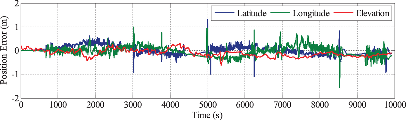
Figure 13. Position errors of MAGNSS/INS integrated navigation.
From Figures 12 and 13, it can be seen that the position solutions of the MAGNSS/INS are almost the same as for PPP/INS. The statistics of the position solutions are shown in Table 4. From the table, it can be seen that the MAGNSS attitude has little effect on the position solutions.
Table 4. Statistics of the position errors.
5. CONCLUSIONS AND DISCUSSION
In this study, the MAGNSS attitude determination method and the MAGNSS/INS integrated navigation are described in detail. A vehicle-mounted test was conducted to evaluate the performances of the proposed algorithms by comparing the solutions with the references derived from the integration of the DGNSS and the navigation-grade INS. The characteristics of the attitude errors of the PPP/INS integration and the advantages of the MAGNSS/INS integration in attitude determination have been demonstrated. The results indicate that when the tactical-grade INS is used, the PPP/INS integrated navigation can achieve high-accuracy position, roll and pitch but low accuracy yaw. The proposed MAGNSS/INS algorithm, using the attitude from MAGNSS, improves the yaw accuracy.
For mobile surveying over a large area, the proposed MAGNSS/INS integration can provide high-accuracy position and attitude using low-grade INS and MAGNSS without a base station. Thus, this method is an alternative to DGNSS/INS integration. As high-grade INS and local base stations are not required, its complexity and cost are significantly decreased.
The INS used in this study is tactical grade. If a lower accuracy INS is used, such as a Micro-Electro-Mechanical-System (MEMS) INS, the improvement of MAGNSS/INS integration relative to PPP/INS integration will be greater.
ACKNOWLEDGEMENT
The authors would like to thank the reviewers for the comments and suggestions that substantially improved this paper.
FINANCIAL SUPPORT
This work was supported by the China National Key R&D Program (Grant No. 2016YFB0501700, 2016YFB0501705) and the National Natural Science Foundation of China (Grant No. 41621091).