


1. Introduction
Nonlinear shear flow instabilities often lead to intermittency, a phenomenon that involves the coexistence of laminar and turbulent flow regions. The resulting turbulent–laminar patterns take either the form of localised turbulent patches surrounded by otherwise laminar flow or, surprisingly more orderly, of coherent stripes that exhibit sharp interfaces tilted with respect to the main direction of the flow. A well-known archetype for coherent intermittency in rotating shear flows is the so-called spiral turbulence (SPT) regime that appears in Taylor–Couette flow (TCF), i.e. the fluid flow between independently rotating coaxial cylinders. The SPT regime consists of a turbulent helix that forms a coil within the apparatus gap with a well-defined pitch and rotates at a fairly constant angular speed. This peculiar flow structure, first discovered in the 1960s (Coles & Van Atta Reference Coles and Van Atta1967) and declared a puzzling phenomenon by Feynman himself (Feynman Reference Feynman1964), had not been reproduced numerically until rather recently by means of very costly direct numerical simulations (DNS) (Dong Reference Dong2009; Meseguer et al. Reference Meseguer, Mellibovsky, Avila and Marques2009b; Dong & Zheng Reference Dong and Zheng2011).
Similar oblique laminar–turbulent stripe patterns are common in other shear flows featuring two extended space directions (Prigent et al. Reference Prigent, Grégoire, Chaté, Dauchot and van Saarloos2002; Duguet, Schlatter & Henningson Reference Duguet, Schlatter and Henningson2010; Tuckerman et al. Reference Tuckerman, Kreilos, Schrobsdorff, Schneider and Gibson2014). For a thorough review on the rich variety of existing intermittent shear flow phenomena, we refer the reader to the monograph by Tuckerman, Chantry & Barkley (Reference Tuckerman, Chantry and Barkley2020) and references therein. Recent attempts at elucidating the stripe formation mechanism have mostly been confined to relatively simple parallel shear flows such as plane Couette or plane Poiseuille flows. Both problems exhibit subcritical transition to turbulence, namely transition in the absence of a linear instability of the base flow, which is best tackled employing dynamical systems theory. In this framework, simple solutions to the Navier–Stokes equations, often called exact coherent structures (ECS), are shown to naturally play a central role in organising the transitional and turbulent dynamics (Kerswell Reference Kerswell2005; Eckhardt et al. Reference Eckhardt, Schneider, Hof and Westerweel2007; Kawahara, Uhlmann & Van Veen Reference Kawahara, Uhlmann and Van Veen2012; Graham & Floryan Reference Graham and Floryan2021).
The last three decades have witnessed overwhelming scientific activity in the search for ECS in many subcritical shear flows (Nagata Reference Nagata1990; Clever & Busse Reference Clever and Busse1992, Reference Clever and Busse1997; Faisst & Eckhardt Reference Faisst and Eckhardt2003; Waleffe Reference Waleffe2003; Wedin & Kerswell Reference Wedin and Kerswell2004), following the discovery of a self-sustained process (SSP) for coherent structures in the absence of linear instability of the laminar flow (Waleffe Reference Waleffe1997). The process, which occurs at relatively short length scales and can therefore be observed in small periodic domains, consists in a cyclic feedback mechanism whereby streamwise vortices generate streaks through the lift-up mechanism, which in turn become unstable to three-dimensional waves that feed energy back into the streamwise vortices (Boberg & Brosa Reference Boberg and Brosa1988; Hamilton, Kim & Waleffe Reference Hamilton, Kim and Waleffe1995; Grossmann Reference Grossmann2000). The instability of the streaks responds to an inviscid mechanism by which three-dimensional waves are strongly amplified at a critical layer, i.e. where the streak speed coincides with the wave speed (Wang, Gibson & Waleffe Reference Wang, Gibson and Waleffe2007; Hall & Sherwin Reference Hall and Sherwin2010; Deguchi & Hall Reference Deguchi and Hall2015).
For relatively small periodic boxes, the relationship between the exact solution and the dynamics is understood to some extent. Of the ECS emanated from saddle-node bifurcations, the lower (or saddle) branch typically dictates the topology and amplitude of flow perturbations that are capable of triggering transition, while the upper (or nodal) branch generally regulates – or at least participates in – the formation of the turbulent set. In the subcritical transition problem, the infinite-dimensional Navier–Stokes phase space typically contains two stable (or metastable) invariant sets: the steady laminar base flow and the chaotic/turbulent state. The basins of attraction of these two sets meet along a codimension-1 manifold, usually known as the edge of chaos (Itano & Toh Reference Itano and Toh2001; Skufca, Yorke & Eckhardt Reference Skufca, Yorke and Eckhardt2006; Schneider et al. Reference Schneider, Gibson, Lagha, De Lillo and Eckhardt2008), where the lower-branch solutions belong. The upper branch ECS are almost always unstable and their participation in the generation of the chaotic set is not easily dissected. Occasionally, however, upper-branch ECS are linearly stable, if only within sufficiently small domains or tightly constrained symmetry conditions, in a neighbourhood of the saddle-node bifurcation (Clever & Busse Reference Clever and Busse1997; Mellibovsky & Eckhardt Reference Mellibovsky and Eckhardt2011, Reference Mellibovsky and Eckhardt2012). In these cases, further theoretical progress can be made as the path towards chaotic dynamics admits a simpler analysis that can draw from a parallel with low-dimensional dynamical systems (Kreilos & Eckhardt Reference Kreilos and Eckhardt2012; Mellibovsky & Eckhardt Reference Mellibovsky and Eckhardt2012; Lustro et al. Reference Lustro, Kawahara, van Veen, Shimizu and Kokubu2019).
Transition and pattern formation in TCF are more involved than for parallel shear flows due to the interplay of shear and rotation (Andereck, Liu & Swinney Reference Andereck, Liu and Swinney1986). A notable difference with respect to merely shear-driven flows is that SPT also persists in the supercritical regime of counter-rotating TCF, beyond the linear instability of the laminar circular Couette flow (Prigent et al. Reference Prigent, Grégoire, Chaté, Dauchot and van Saarloos2002; Meseguer et al. Reference Meseguer, Mellibovsky, Avila and Marques2009b). Therefore, both the shear and the centrifugal instabilities contribute their share to the generation of streamwise vorticity, but this fact has gone largely unnoticed in the literature, where the origin of the stripe can be solely explained by the stability of both the basic flow and the autonomous vortex emerged from the SSP. The mechanism we are interested in is also fundamentally different from that of wavy vortex flow (WVF) (Martinand, Serre & Lueptow Reference Martinand, Serre and Lueptow2014; Dessup et al. Reference Dessup, Tuckerman, Wesfreid, Barkley and Willis2018), for which the roll–streak system is almost exclusively driven by the centrifugal instability of circular Couette flow (CCF), with shear playing but an accessory and marginal part in the sustainment.
The aim of this paper is to investigate the dynamics induced by ECS driven by the SSP and to ascertain whether they may be held responsible for the formation of the SPT regime observed in the centrifugally unstable region of parameter space. The most natural place to look for nonlinear solutions is at the linear critical point of the base flow, CCF in our case. However, the nonlinear spiral solutions thus identified by Meseguer et al. (Reference Meseguer, Mellibovsky, Avila and Marques2009a) are only very mildly subcritical, which implies that it is the centrifugal instability rather than the SSP that drives them. A wealth of solutions predicted by weakly nonlinear theory (Chossat & Iooss Reference Chossat and Iooss1994) followed the discovery of the subcritical spirals (Deguchi & Altmeyer Reference Deguchi and Altmeyer2013), but none contributed to enlarging the known region of subcriticality. Shortly after, however, a highly subcritical three-dimensional rotating-wave solution was found by Deguchi, Meseguer & Mellibovsky (Reference Deguchi, Meseguer and Mellibovsky2014), although its dynamical relevance was not investigated.
As noted earlier, the computation of laminar–turbulent banded patterns is very costly, such that using narrow orthogonal domains suitably tilted to align with the stripes has been decisive to the study of this kind of laminar–turbulent patterns (Barkley & Tuckerman Reference Barkley and Tuckerman2005; Shi, Avila & Hof Reference Shi, Avila and Hof2013; Reetz, Kreilos & Schneider Reference Reetz, Kreilos and Schneider2019; Paranjape, Duguet & Hof Reference Paranjape, Duguet and Hof2020). The approach is easily undertaken for parallel shear flows, as a mere change in the direction of the base flow suffices, but more fundamental code modifications are necessary for cylindrical and annular geometries. The required coordinate change was generalised by Deguchi & Altmeyer (Reference Deguchi and Altmeyer2013) to compute ECS in parallelogram-shaped domains wrapped within an annular geometry. Since their method of directly solving the nonlinear algebraic equations was only applicable to travelling-wave solutions, developing a DNS code in generalised parallelogram-shaped periodic domains is requisite to efficiently capture SPT dynamics, but has hitherto not been attempted to our best knowledge.
The outline of the paper is as follows. The problem formulation is given in § 2, alongside a description of the generalised parallelogram-shaped domain, its application to the spectral space discretisation, and the numerical methods employed for evolving the equations in time, and the coupling of the time stepper with a Poincaré–Newton–Krylov solver. Then § 3 briefly summarises the geometrical and physical parameters used for the numerical calculations, and justifies the specific choice of the domain shape. Since the rotating-wave solutions found by Deguchi et al. (Reference Deguchi, Meseguer and Mellibovsky2014) were computed in a classical orthogonal small periodic domain, the initial task in § 4 is the exploration of bifurcation scenarios leading to solutions of the same family in small parallelogram domains. In § 5, the dynamical relevance of the solution is first analysed in the subcritical regime to identify the SSP and the onset of chaotic dynamics. The possible relevance of these solutions to the supercritical SPT regime is then discussed. Finally, the main findings are summarised in § 6 along with concluding remarks.
2. Formulation of the problem
Consider an incompressible fluid of dynamic viscosity  $\mu$ and density
  $\varrho$ (kinematic viscosity
  $\nu =\mu /\varrho$) completely filling the gap between two concentric rotating cylinders whose inner and outer radii and angular velocities are
  $r^*_{i}$,
  $r^*_{o}$ and
  $\varOmega _{i}$,
  $\varOmega _{o}$, respectively. A full set of independent dimensionless parameters characterising the problem are the radius ratio
  $\eta =r^*_{i}/r^*_{o}$, which fixes the geometry of the annulus, and the CCF inner and outer Reynolds numbers
  ${{R}_{i}}=dr^*_{i}\varOmega _{i}/\nu$ and
  ${{R}_{o}}=dr^*_{o}\varOmega _{o}/\nu$, where
  $d=r^*_{o}-r^*_{i}$ is the gap between the cylinders. Henceforth, all variables will be rendered dimensionless using
  $d$,
$d$,  $d^2/\nu$ and
  $\nu ^2/d^2$ as units for space, time and the reduced pressure (
 $p=p^*/\varrho$), respectively. The Navier–Stokes equation, and the incompressibility and the zero axial net massflux conditions become
 $$\begin{gather} \partial_{t}\boldsymbol{v} + (\boldsymbol{v}\boldsymbol{\cdot}\boldsymbol{\nabla})\boldsymbol{v} ={-}\boldsymbol{\nabla} p + \nabla^{2}\boldsymbol{v} + f\,\hat{{\boldsymbol{z}}}, \end{gather}$$
 $$\begin{gather}\boldsymbol{\nabla}\boldsymbol{\cdot}\boldsymbol{v} = 0, \end{gather}$$
 $$\begin{gather}Q(\boldsymbol{v}) = \int_0^{2{\rm \pi}}{\int_{r_{i}}^{r_{o}}{(\boldsymbol{v}\boldsymbol{\cdot}\hat{{\boldsymbol{z}}})\,r\,{\rm d}r\,{\rm d}\theta}} = 0, \end{gather}$$
where the axial forcing term  $f=f(t)$ in (2.1) is instantaneously adjusted to fulfil the constraint imposed by (2.3),
  $\boldsymbol {v}=(U,V,W)=U\,\hat {{\boldsymbol {r}}} + V\,\hat {{\boldsymbol { \theta }}} + W\,\hat {{\boldsymbol {z}}}$ is the velocity of the fluid expressed in cylindrical coordinates
  $(r,\theta,z)$, which satisfies no-slip boundary conditions at the cylinder walls
 \begin{equation} \boldsymbol{v}|_{r=r_i}=(0,{{R}_{i}},0),\quad \boldsymbol{v}|_{r=r_{o}}=(0,{{R}_{o}},0), \end{equation}
with
 \begin{equation} r_i=\frac{r^*_i}{d} = \frac{\eta}{1-\eta}, \quad r_o=\frac{r^*_o}{d} = \frac{1}{1-\eta}, \end{equation}
the non-dimensional inner and outer radii, respectively. The basic, laminar and steady CCF is
 \begin{equation} \boldsymbol{v}_{b} = U_{b}\,\hat{{\boldsymbol{r}}} + V_{b}\,\hat{{\boldsymbol{ \theta}}} + W_{b}\,\hat{{\boldsymbol{z}}} = \left(Ar+\frac{B}{r}\right)\,\hat{{\boldsymbol{ \theta}}}, \quad p_{b}(r)=\int\frac{V_{b}^2}{r} \,{\rm d}r, \quad f_{b} = 0, \end{equation}
with  $A=({{R}_{o}}-\eta {{R}_{i}})/(1+\eta )$ and
  $B=\eta ({{R}_{i}}-\eta {{R}_{o}})/[(1-\eta )(1-\eta ^2)]$. In what follows we express the velocity and pressure fields as
 \begin{equation} \boldsymbol{v} = \boldsymbol{v}_{b}(r) + \boldsymbol{u}(r,\theta,z;t), \quad p=p_{b}(r) + q(r,\theta,z;t). \end{equation}
The fields  $q$ and
  $\boldsymbol {u}= u\,\hat {{\boldsymbol {r}}} + v\,\hat {{\boldsymbol { \theta }}} + w\,\hat {{\boldsymbol {z}}}$ are the deviations from the equilibrium CCF solution that, after formal substitution of (2.7a,b) into (2.1), satisfy
 $$\begin{gather} \partial_t{\boldsymbol u} ={-}\boldsymbol{\nabla} q + \nabla^2{\boldsymbol u}-({\boldsymbol v}_{b} \boldsymbol{\cdot} \boldsymbol{\nabla}){\boldsymbol u}-({\boldsymbol u} \boldsymbol{\cdot} \boldsymbol{\nabla}){\boldsymbol v}_{b}-({\boldsymbol u} \boldsymbol{\cdot} \boldsymbol{\nabla}){\boldsymbol u} + f\,\hat{{\boldsymbol{z}}}, \end{gather}$$
 $$\begin{gather}\boldsymbol{\nabla} \boldsymbol{\cdot} {\boldsymbol u} = 0, \end{gather}$$
 $$\begin{gather}Q(\boldsymbol{u}) = 0. \end{gather}$$
Although this solenoidal boundary value problem is naturally formulated in cylindrical polar coordinates  $(r,\theta,z)$, the coherent flows addressed in this work are better captured and more efficiently represented numerically on parallelogram domains such as the one depicted in figure 1. These types of domains have been recently vindicated as minimal flow units to capture mixed spiral modes and rotating–travelling waves with arbitrary axial-azimuthal wavefront orientation in TCF (Deguchi & Altmeyer Reference Deguchi and Altmeyer2013; Deguchi & Hall Reference Deguchi and Hall2015; Ayats et al. Reference Ayats, Deguchi, Mellibovsky and Meseguer2020a). The parallelogram domain is bounded by two consecutive (
 $2{\rm \pi}$-shifted) wavefront loci and might be naturally parametrised by introducing the new coordinates
 \begin{equation} \xi = n_1\theta + k_1 z,\quad \zeta = n_2\theta + k_2 z, \end{equation}
or, conversely,
 \begin{equation} \theta = \frac{k_2 \xi - k_1 \zeta}{n_1k_2-n_2k_1},\quad z = \frac{-n_2 \xi + n_1 \zeta}{n_1k_2-n_2k_1}. \end{equation}
Henceforth, we reformulate the boundary value problem ((2.8)–(2.9)) within the parallelogram assuming the pressure and velocity fields  $q$ and
  $\boldsymbol {u}$ are
  $2{\rm \pi}$-periodic in the two new coordinates
  $\xi$ and
  $\zeta$, thus satisfying
 $$\begin{gather} q(r,\xi+2{\rm \pi},\zeta;t) = q(r,\xi,\zeta+2{\rm \pi};t) = q(r,\xi,\zeta;t), \end{gather}$$
 $$\begin{gather}\boldsymbol{u}(r,\xi+2{\rm \pi},\zeta;t) = \boldsymbol{u}(r,\xi,\zeta+2{\rm \pi};t) = \boldsymbol{u}(r,\xi,\zeta;t). \end{gather}$$
In what follows, we numerically discretise  $q$ and
  $\boldsymbol {u}$ within the annular–parallelogram domain
 \begin{equation} (r,\xi,\zeta) \in \left[r_{i},r_{o}\right] \times[0,2{\rm \pi}]\times[0,2{\rm \pi}], \end{equation}
where the inner and outer radii of the cylinders are explicitly given in (2.5a,b). We characterise flows by their associated normalised torque at the inner and outer cylinders,  $\tau _{i}$ and
  $\tau _{o}$,
 \begin{equation} \tau_{i, o} = \left. 1+\frac{\partial_r(r^{{-}1}\bar{v})}{\partial_r(r^{{-}1}v_{b})}\right|_{r=r_{i},r_{o}}, \end{equation}
where  $\bar {v}$ is the averaged azimuthal velocity in the angular and axial directions. Similarly, we will also characterise the flows by the normalised kinetic energy of the perturbation velocity field,
 \begin{equation} \kappa = \frac{E(\boldsymbol{u})}{E(\boldsymbol{v}_b)}, \end{equation}
where  $E(\boldsymbol {v})$ is the volume-averaged kinetic energy of any velocity field
  $\boldsymbol {v}$, defined as
 \begin{equation} E(\boldsymbol{v}) = \frac{1}{2\mathcal{V}} \int_{0}^{2{\rm \pi}}{\int_{0}^{2{\rm \pi}}{\int_{r_{i}}^{r_{o}}{\boldsymbol{v}\boldsymbol{\cdot}\boldsymbol{v}\, r\,\mathrm{d}r}\,\mathrm{d}\xi}\,\mathrm{d}\zeta}, \quad \mathcal{V} = \int_{0}^{2{\rm \pi}} \int_{0}^{2{\rm \pi}} \int_{r_{i}}^{r_{o}} r\,\mathrm{d}r\,\mathrm{d}\xi\,\mathrm{d}\zeta. \end{equation}
With these definitions,  $\tau _{i}=\tau _{o}=1$ and
  $\kappa =0$ for CCF.

Figure 1. Sketch of the parallelogram domain introducing the new variables  $(\xi,\zeta )$ that replace the usual azimuthal and axial coordinates
  $(\theta,z)$.
2.1. Direct numerical simulations in the annular–parallelogram domain
The nonlinear boundary value problem ((2.8)–(2.9)) is discretised using a solenoidal Petrov–Galerkin scheme formerly formulated by Meseguer et al. (Reference Meseguer, Avila, Mellibovsky and Marques2007), and suitably adapted to the annular–parallelogram domain (2.15). In the transformed domain, the solenoidal velocity perturbation is approximated by means of a Fourier  $\times$ Fourier
  $\times$ Chebyshev spectral expansion
  ${\boldsymbol u}_{s}$ of order
  $N \times L \times M$ in
  $\xi \times \zeta \times r$, respectively, of the form
 \begin{equation} {\boldsymbol u}_{s}(r,\xi,\zeta;t)=\sum_{\ell={-}L}^{L} \sum_{n={-}N}^{N} \sum_{m=0}^{M} a_{\ell nm}^{(1)}(t) \boldsymbol{\varPhi}_{\ell nm}^{(1)}(r,\xi,\zeta)+a_{\ell nm}^{(2)}(t) \boldsymbol{\varPhi}_{\ell nm}^{(2)}(r,\xi,\zeta). \end{equation}
Our aim here is to derive the dynamical system satisfied by the coefficients  $a_{\ell nm}^{(\imath )}(t)$, as symbolically represented by the
  $2\times (M+1)\times (2L+1)\times (2N+1)$-dimensional state vector
  $\boldsymbol {a}(t)$. The binary superindex
  $\imath =\{1,2\}$ and the factor 2 in the count of unknowns follow from the two degrees of freedom per grid point that remain after taking into consideration that the three velocity components are not independent, but linked by the solenoidal condition. The vector fields
  $\boldsymbol {\varPhi }_{\ell n m}^{(\imath )}$ constitute the elements of the trial basis of solenoidal vector fields of the form
 \begin{equation} \boldsymbol{\varPhi}_{\ell n m}^{(\imath)}(r,\xi,\zeta) = \mathrm{e}^{\mathrm{i}(n\xi+\ell\zeta)} \boldsymbol{u}_{\ell nm}^{(\imath)}(r) = \mathrm{e}^{\mathrm{i}(n\xi+\ell\zeta)} (u_{\ell n m}^{(\imath)},v_{\ell n m}^{(\imath)},w_{\ell n m}^{(\imath)}), \end{equation}
where  $u_{\ell n m}^{(\imath )}$,
  $v_{\ell n m}^{(\imath )}$ and
  $w_{\ell n m}^{(\imath )}$ are the radial, azimuthal and axial components of
  $\boldsymbol {u}_{\ell nm}^{(\imath )}(r)$, respectively. Each element of the trial basis satisfies the divergence-free condition (2.9) that, in the
  $(r,\xi,\zeta )$ variables, explicitly reads
 \begin{equation} \left(\partial_r + \frac{1}{r}\right) u_{\ell nm}^{(\imath)} + \frac{\mathrm{i}}{r}\left(n_1n + n_2\ell \right)v_{\ell n m}^{(\imath)} + {\rm i}\left(k_1n+k_2\ell \right) w_{\ell nm}^{(\imath)}=0. \end{equation}
Since  $\boldsymbol {u}$ represents the perturbation of the velocity field, it must therefore vanish at the inner (
 $r=r_{i}$) and outer (
 $r=r_{o}$) walls of the cylinders. Therefore,
  $\boldsymbol {\varPhi }_{\ell n m}^{(\imath )}$ must also satisfy the homogeneous boundary conditions
 \begin{equation} \boldsymbol{\varPhi}_{\ell n m}^{(\imath)}(r_{i},\xi,\zeta;t)=\boldsymbol{\varPhi}_{\ell n m}^{(\imath)}(r_{o},\xi,\zeta;t)=\boldsymbol{0}. \end{equation}
In what follows, we define the transformed radial coordinate
 \begin{equation} x(r) = 2r-\frac{1+\eta}{1-\eta}, \end{equation}
that maps the radial domain  $r\in [r_{i},r_{o}]$ to the interval
  $x\in [-1,1]$. In addition, we define the radial functions
 \begin{equation} {h}_m(r)=(1-x^2){T}_m(x),\quad {g}_m(r)=(1-x^2)^2{T}_m(x), \end{equation}
where  ${T}_m(x)$ is the Chebyshev polynomial of degree
  $m$. Finally, we introduce the Chebyshev weight function
  ${w}(x)=(1-x^2)^{-1/2}$, defined over the interval
  $(-1,1)$. The functions introduced in (2.24a,b) satisfy
 \begin{equation} {h}_m(r_{i})={h}_m(r_{o})={g}_m(r_{i})={g}_m(r_{o})={\rm D}{g}_m(r_{i})={\rm D}{g}_m(r_{o})=0, \end{equation}
where  ${\rm D}$ stands for the radial derivative
  ${\rm d}/{\rm d}r$. The solenoidal spectral method consists in devising complete sets of vector fields (trial functions) satisfying (2.21) and (2.22). For
  $n n_1+\ell n_2 = 0$, two such vector fields are
 \begin{equation} \boldsymbol{u}_{\ell n m}^{(1)}(r)=(0,{h}_m,0),\quad \boldsymbol{u}_{\ell n m}^{(2)}(r)=( -\mathrm{i}(n k_1+\ell k_2) r {g}_m,0,{\rm D}[r {g}_m]+{g}_m), \end{equation}
with the third component of  $\boldsymbol {u}_{\ell n m}^{(2)}$ replaced by
  ${h}_m$ whenever
  $n k_1+\ell k_2=0$. Finally, for
  ${n n_1+\ell n_2 \neq 0}$, the solenoidal basis is
 $$\begin{gather} \boldsymbol{u}_{\ell nm}^{(1)}(r) =(-\mathrm{i}(n n_1+\ell n_2) {g}_m , {\rm D}[r {g}_m] , 0), \end{gather}$$
 $$\begin{gather}\boldsymbol{u}_{\ell nm}^{(2)}(r) =(0,-\mathrm{i} (n k_1+\ell k_2) r{h}_m , \mathrm{i}(n n_1+\ell n_2) {h}_m), \end{gather}$$
except that the third component of  $\boldsymbol {u}_{\ell nm}^{(2)}$ is replaced by
  ${h}_m$ when
  $n k_1+\ell k_2=0$. The Petrov–Galerkin solenoidal weak formulation is completed by introducing the Hermitian product of two arbitrary solenoidal trial and dual fields
  $\boldsymbol {\varPhi }$ and
  $\boldsymbol {\varPsi }$, respectively, over the annular–parallelogram domain (2.15)
 \begin{equation} (\boldsymbol{\varPsi},\boldsymbol{\varPhi})=\int_{0}^{2{\rm \pi}}\int_{0}^{2{\rm \pi}} \int_{r_{i}}^{r_{o}} \; \boldsymbol{\varPsi}^{\dagger} \boldsymbol{\cdot} \boldsymbol{\varPhi} \;r\,\mathrm{d}r\,\mathrm{d}\xi\,\mathrm{d}\zeta. \end{equation}
Accordingly, we consider the dual basis for the projection space. In particular, the basis for the case  $n n_1+\ell n_2 = 0$ is
 $$\begin{gather} \boldsymbol{\tilde{u}}_{\ell 0m}^{(1)}(r) = {w}(0, r {h}_m, 0), \end{gather}$$
 $$\begin{gather}\boldsymbol{\tilde{u}}_{\ell 0m}^{(2)}(r) = r^{{-}2}{w} (\mathrm{i}(n k_1+\ell k_2) {g}_m,0, {\rm D}_+{g}_m +2r^{{-}1}(1-x^2+rx){h}_m), \end{gather}$$
where  ${\rm D}_+={\rm D}+r^{-1}$, and the third component of
  $\boldsymbol {\tilde {u}}_{\ell 0m}^{(2)}$ is replaced by
  $r {h}_m$ if
  $n k_1+\ell k_2=0$. Similarly, the basis for the case
  $n n_1+\ell n_2 \neq 0$ is
 $$\begin{gather} \boldsymbol{\tilde{u}}_{\ell n m}^{(1)}(r) = {w} ((n n_1+\ell n_2)\,r{g}_m , r{\rm D}_+[r {g}_m]+2xr^2{h}_m ,0), \end{gather}$$
 $$\begin{gather}\boldsymbol{\tilde{u}}_{\ell n m}^{(2)}(r) = {w} (0,i (n k_1+\ell k_2) r^2{h}_m,-i (n n_1+\ell n_2)\,r{h}_m). \end{gather}$$
These projection basis elements contain the Chebyshev weight function  ${w}(x)$ so that the resulting radial integration involved in (2.29) can be computed exactly by suitable quadrature formulae (Moser, Moin & Leonard Reference Moser, Moin and Leonard1983; Meseguer et al. Reference Meseguer, Avila, Mellibovsky and Marques2007; Canuto et al. Reference Canuto, Hussaini, Quarteroni and Zang2007, Reference Canuto, Hussaini, Quarteroni and Zang2010; Meseguer Reference Meseguer2020).
Formal substitution of the spectral expansion (2.19) into (2.8), followed by Hermitian projection onto each one of the dual basis elements leads to
 \begin{equation} (\boldsymbol{\varPsi}_{\ell n m}^{(\imath)} , \partial_t{\boldsymbol u}_{S}) = (\boldsymbol{\varPsi}_{\ell n m}^{(\imath)} , \nabla^2{\boldsymbol u}-({\boldsymbol v}_{b} \boldsymbol{\cdot} \boldsymbol{\nabla}){\boldsymbol u}-({\boldsymbol u} \boldsymbol{\cdot} \boldsymbol{\nabla}){\boldsymbol v}_{b}-({\boldsymbol u} \boldsymbol{\cdot} \boldsymbol{\nabla}){\boldsymbol u} + f\,\hat{{\boldsymbol{z}}}),\end{equation}
for  $\ell = -L,\ldots,L,\, n=-N,\ldots,N$,
  $m = 0,\ldots, M$ and
  $\imath =1,2$. The pressure deviation field drops upon projection,
  $(\boldsymbol {\varPsi }_{\ell n m}^{(\imath )},\boldsymbol {\nabla } q)=0$, by virtue of Stokes’ theorem and has therefore been omitted. Equation (2.34), subject to the constraint (2.3), constitutes a dynamical system
 $$\begin{gather} {\mathsf{A}}_{\ell nm(\jmath)}^{pqr(\imath)} \, \dot{a}_{pqr}^{(\jmath)} = {\mathsf{B}}_{\ell n m(\jmath)}^{pqr(\imath)} \, a_{pqr}^{(\jmath)} + \left[\boldsymbol{N}(\boldsymbol{a})\right]_{\ell n m}^{(\imath)} + f{F}_{\ell nm}^{(\imath)}, \end{gather}$$
 $$\begin{gather}Q^r a_{00r}^{(2)} = 0, \end{gather}$$
for the axial forcing  $f(t)$ and amplitudes
  $a_{\ell n m}^{(\imath )}(t)$, where repeated indices must be interpreted following the index summation convention. The zero-net-massflux constraint reduces to a mere linear equation for the
  $n=l=0$,
  $\imath =2$ coefficients upon substitution of (2.19). The quadratic form
  $\left[\boldsymbol{N}(\boldsymbol{a})\right]_{\ell n m}^{(\imath)}$ appearing in (2.35) corresponds to the projection of the nonlinear convective term,
  $(\boldsymbol {\varPsi }_{\ell n m}^{(\imath )} , ({\boldsymbol u} \boldsymbol {\cdot } \boldsymbol {\nabla }){\boldsymbol u})$, which is computed pseudospectrally using Orszag's
  $3/2$-dealiasing rule (Canuto et al. Reference Canuto, Hussaini, Quarteroni and Zang2007, Reference Canuto, Hussaini, Quarteroni and Zang2010). Overall, the resulting stiff system of ordinary differential equations is integrated in time by means of a fourth-order linearly implicit backwards differentiation scheme with explicit polynomial extrapolation of the nonlinear terms, conveniently started with a fourth-order Runge–Kutta method.
2.2. Computation and stability analysis of invariant solutions
In the  $(\xi,\zeta )$ coordinate system, a travelling wave is represented by the spectral expansion
 \begin{align} &{\boldsymbol u}_{s}(r,\xi,\zeta;t)=\nonumber\\ &\qquad =\displaystyle{\sum_{\ell={-}L}^{L} \sum_{n={-}N}^{N} \sum_{m=0}^{M} [\check{a}_{\ell nm}^{(1)} \boldsymbol{\varPhi}_{\ell nm}^{(1)}(r,\xi,\zeta) + \check{a}_{\ell nm}^{(2)} \boldsymbol{\varPhi}_{\ell nm}^{(2)}(r,\xi,\zeta)] \mathrm{e}^{\mathrm{i} n(\xi-c_\xi t)}\mathrm{e}^{\mathrm{i} \ell(\zeta-c_\zeta t)}}, \end{align}
where  $c_\xi$ and
  $c_\zeta$ are the unknown wave speed components in the
  $\xi$ and
  $\zeta$ directions, respectively, so that the Fourier–Chebyshev spectral coefficients of this particular type of solution read
 \begin{equation} a_{\ell nm}^{(\imath)}(t) = \check{a}_{\ell nm}^{(\imath)} \mathrm{e}^{-\mathrm{i} n c_\xi t}\mathrm{e}^{- \mathrm{i} \ell c_\zeta t}, \end{equation}
with the complex constant  $\check {a}_{\ell nm}^{(\imath )}$ representing the wave shape unambiguously except for arbitrary rotations and shifts. In this case, formal introduction of expansion (2.37) in (2.8) followed by Hermitian projection leads to the following system of nonlinear algebraic equations for the travelling wave coefficients
  $\check {a}_{\ell nm}^{(\imath )}$ (
 $\check {\boldsymbol {a}}$ for brevity):
 $$\begin{gather} \left[{\mathsf{B}}_{\ell n m(\jmath)}^{pqr(\imath)} + \mathrm{i} (n c_\xi + \ell c_\zeta) {\mathsf{A}}_{\ell n m (\jmath)}^{pqr(\imath)}\right] \check{a}_{pqr}^{(\jmath)} + \left[\boldsymbol{N}(\boldsymbol{\check{a}})\right]_{\ell n m}^{(\imath)} + \check{f}{F}_{\ell n m}^{(\imath)} = 0, \end{gather}$$
 $$\begin{gather}Q^r \check{a}_{00r}^{(2)} = 0, \end{gather}$$
where  $\check {\boldsymbol {a}}$ appearing in the nonlinear term is the state vector representing the Fourier–Chebyshev coefficients
  $\check {a}_{\ell nm}^{(\imath )}$ of the travelling wave, and
  $\check {f}$ is the axial pressure gradient required to enforce the zero-net-flux condition. The azimuthal and axial degeneracy of solutions, associated with drift speeds
  $c_\xi$ and
  $c_\zeta$, is removed using two additional phase constraints in the same way as is done for the computation of rotating–travelling waves in pipe flow (Mellibovsky & Eckhardt Reference Mellibovsky and Eckhardt2011). The system is solved using a matrix-free Newton–Krylov method (Kelley Reference Kelley2003), implicitly using the generalized minimal residual method (GMRES) as a matrix-free solver (Trefethen & Bau Reference Trefethen and Bau1997). The converged nonlinear solutions are tracked in parameter space using pseudoarclength continuation schemes (Kuznetsov Reference Kuznetsov2004).
The linear stability of a travelling-wave solution of (2.39) is formulated by adding disturbances of very small amplitude  $|\varepsilon _{\ell n m}^{(\imath )}|\ll |\check {a}_{\ell nm}^{(\imath )}|$ to its Fourier–Chebyshev coefficients following
 $$\begin{gather} a_{\ell nm}^{(\imath)}(t) = (\check{a}_{\ell nm}^{(\imath)}+\varepsilon_{\ell n m}^{(\imath)} \mathrm{e}^{\sigma t})\mathrm{e}^{-\mathrm{i} n c_\xi t}\mathrm{e}^{- \mathrm{i} \ell c_\zeta t}, \end{gather}$$
 $$\begin{gather}f(t) = \check{f} + \phi \mathrm{e}^{\sigma t}, \end{gather}$$
and the forcing perturbation  $|\phi |\ll |\check {f}|$ is such that coefficient perturbations comply also with the zero-massflux condition
  $Q^r \varepsilon _{00r}^{(2)}=0$. Formal substitution of the perturbed solution (2.41) in (2.35), and subsequent neglect of quadratic perturbation terms, leads to the constrained generalised eigenvalue problem
 $$\begin{gather} \left( \sigma -\mathrm{i} n c_\xi - \mathrm{i} \ell c_\zeta \right){\mathsf{A}}_{\ell n m(\jmath)}^{p q r(\imath)}\varepsilon_{pqr}^{(\jmath)} = {\mathsf{B}}_{\ell n m(\jmath)}^{p q r(\imath)}\varepsilon_{pqr}^{(\jmath)} + \left[\boldsymbol{D}_{\boldsymbol{a}}\boldsymbol{N}(\check{\boldsymbol{a}})\right]_{\ell n m(\jmath)}^{p q r(\imath)}\!\varepsilon_{pqr}^{(\jmath)} + \phi {F}_{\ell n m}^{(\imath)}, \end{gather}$$
 $$\begin{gather}Q^r \varepsilon_{00r}^{(2)} = 0, \end{gather}$$
where  $\boldsymbol{D}_{\boldsymbol{a}}\boldsymbol{N}(\check {\boldsymbol {a}})$ is the linear action of the Jacobian of
  $\boldsymbol{N}$ evaluated at the travelling-wave solution
  $\check {\boldsymbol {a}}$, and
  $(p,q,r,\jmath ) \in [0,L]\times [-N,N]\times [0,M]\times \{1,2\}$. This linear action therefore allows formulation of the generalised eigenvalue problem (2.43) in a matrix-free form, so that Arnoldi methods (Trefethen & Bau Reference Trefethen and Bau1997) can be applied to compute the leading eigenvalues
  $\sigma _j$ and their associated eigenvectors
  $\boldsymbol {\varepsilon }_j=\{\varepsilon _{\ell m n}^{(\imath )}\}_j$.
To compute relative periodic orbits (i.e. modulated travelling waves) beyond their region of linear stability, a Poincaré–Newton–Krylov method is devised. The method is essentially an adaptation of the one used for the computation of modulated travelling waves in plane Poiseuille flow (Mellibovsky & Meseguer Reference Mellibovsky and Meseguer2015). In this case, the method solves the nonlinear system of equations resulting from root finding for the map defined by consecutive crossings of a Poincaré section  $\boldsymbol{P}$, as follows:
 \begin{equation} \boldsymbol{a} \rightarrow \tilde{\boldsymbol{a}} = \boldsymbol{P}(\boldsymbol{a})= \boldsymbol{\mathsf{T}}(\Delta \xi,\Delta \zeta) \boldsymbol{\varphi}(\boldsymbol{a};{T}), \end{equation}
where  $\boldsymbol {\varphi }(\boldsymbol {\cdot };t)$ is the action of the uniparametric group or flow generated by (2.35),
  ${T}$ is the modulation period of the relative periodic orbit, and
 \begin{equation} \left[\boldsymbol{\mathsf{T}}(\Delta \xi,\Delta \zeta)\boldsymbol{a}\right]_{\ell n m}^{(\imath)} = \mathrm{e}^{-\mathrm{i} n \Delta \xi }\mathrm{e}^{-\mathrm{i} \ell \Delta \zeta}a_{\ell n m}^{(\imath)} \end{equation}
is a double-shift operator, removing the drift of the relative periodic orbit in the two homogeneous parallelogram coordinates  $\xi$ and
  $\zeta$. Finally, the above-described time-stepping formulation, as well as the travelling wave and relative periodic orbit solvers, are enforced to satisfy zero net flux condition for the perturbation field.
3. Choice of geometrical and physical parameters
The present study is done for the same cylinder radius ratio of  $\eta =0.883$ as employed by Andereck et al. (Reference Andereck, Liu and Swinney1986) in their Taylor–Couette apparatus. The outer Reynolds number is fixed to
  ${{R}_{o}}=-1200$, at which Meseguer et al. (Reference Meseguer, Mellibovsky, Avila and Marques2009b) found numerically that SPT is sustained within sufficiently large domains for values of the inner cylinder Reynolds number ranging in
  ${{R}_{i}} \in [540, 640]$ (see line
  $\varGamma _2$ in figure 3 of that paper). Below the lower threshold for SPT, spot-like intermittency is observed for an interval and, beneath it, a regime of interpenetrating-spirals that prevails in the range
  ${{R}_{i}} \in [450, 480]$.
The critical point above which CCF becomes linearly unstable with respect to non-axisymmetric perturbations occurs at  ${{R}_{i}}=447.35$. The bifurcating nonlinear spiral-wave solution branches found by Meseguer et al. (Reference Meseguer, Mellibovsky, Avila and Marques2009a) can only be continued down to
  ${{R}_{i}}=445.65$, which makes them qualify as only mildly subcritical. While none of the mixed-mode solutions detected by Deguchi & Altmeyer (Reference Deguchi and Altmeyer2013) reached this value of
  ${{R}_{i}}$, the subcritical rotating waves computed by Deguchi et al. (Reference Deguchi, Meseguer and Mellibovsky2014) do indeed exist in a much wider region of the linearly stable regime, extending to as low as
  ${{R}_{i}}>377.3$.
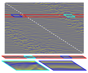
Figure 2(a) shows radial vorticity,  ${\omega _r = (\boldsymbol {\nabla } \times \boldsymbol {v})_r}$, colourmaps for a snapshot of the statistically steady SPT obtained at
  ${R}_{i}=600$ in a sufficiently large computational domain following Meseguer et al. (Reference Meseguer, Mellibovsky, Avila and Marques2009b). The unwrapped domain is a rectangle in the
  $\theta$–
 $z$ plane as usually employed in SPT calculations, and its height-to-gap aspect ratio is
  $\varLambda \approx 31.4$ (corresponding to an axial wavenumber
  $k = 2{\rm \pi} /\varLambda = 0.2$). Within the turbulent stripe, wavy vortices of relatively short axial and azimuthal wavelength emerge. These small-scale flow structures seem to decorrelate rather fast along the spiral slope direction. This statistical property of SPT suggests that a narrow periodic domain winding horizontally around the full apparatus gap but sheared to preserve the tilt of the spiral (dashed white line in figure 2a) would in principle suffice to capture minimally its main topological and dynamical features.

Figure 2. Instantaneous fields of statistically steady states obtained with DNS for  $(\eta,{{R}_{o}},{{R}_{i}})=(0.883,-1200,600)$. All panels show radial vorticity
  $\omega _r\in [-4000,4000]$ colourmaps at the intermediate radius
  $r_{m} = (r_{i}+r_{o})/2 \approx 8.05$. (a) The SPT in the full orthogonal domain of periodic aspect ratio
  $\varLambda =31.4$, with spectral resolution
  $(L,N,M) = (322,322,42)$ (see Supplementary Movie 1 available at https://doi.org/10.1017/jfm.2022.828). The white dashed line indicates the tilt of the stripe and of the minimal narrow domain that can capture SPT (solid red enclosure). (b) The SPT in a narrow long parallelogram domain
  $(n_1,k_1,n_2,k_2)=(1,0.2,0,4.5)$ with resolution
  $(L,N,M) = (18,322,42)$ (see Supplementary Movie 2). The solid cyan parallelogram delimits the minimal domain required for self-sustained turbulent dynamics and used throughout the paper. (c) Turbulent (i) and laminar (ii) snapshots at different time instants along the same simulation within a narrow and short parallelogram domain
  $(n_1,k_1,n_2,k_2)=(10,2,0,4.5)$, using
  $(L,N,M) = (18,32,42)$ spectral modes (see Supplementary Movie 3).
In fact, a localised turbulent stripe arises when DNS is performed in an azimuthally long but axially narrow parallelogram domain such as shown in figure 2(b), whose comparative size is indicated in figure 2(a) as the enclosure bound by a red line. The corresponding generalised wavenumbers for this domain (see figure 1) were chosen as follows. First, we note that the pitch of SPT is enforced by the dimensions of the full domain through the ratio  $k/n=2{\rm \pi} /\varLambda$. A periodic parallelogram domain that can sustain spirals of the same pitch must have the slope of two of its sides prescribed by azimuthal and axial wavenumbers keeping the same ratio
  $k_1/n_1=k/n=0.2$. Picking
  $n_1=1$, and therefore
  $(n_1,k_1)=(1,0.2)$, the parallelogram domain winds exactly once around the apparatus circumference, with its two opposing sides that are aligned with the slope of the spiral falling on the same helical surface. The other pair of sides, defined by the values
  $(n_2,k_2)$, can be chosen arbitrarily at this stage. For simplicity we take
  $n_2=0$, thus forcing the parallelogram to extend horizontally and align with the azimuthal coordinate
  $\xi \equiv \theta$. Notice that the axial height of the domain is then simply specified as
  $2{\rm \pi} /k_2$. Inspecting the typical size of flow structures in figure 2(a), shows that
  $k_2=4.5$ is an adequate choice for the narrow domain size to fit exactly one streak most of the time.
We note here that in the full domain, the symmetry of the system in the axial direction allows for a turbulent spiral band structure with an opposite tilt. However, in the narrow but long parallelogram domain, the symmetry is broken. The choice of the wavenumber ratio  $k_1/n_1=0.2$ makes the realisation of the opposite spiral impossible, which could be computed using instead the wavenumber ratio
  $k_1/n_1=-0.2$.
Finally, if the focus is to be placed exclusively on the small-scale flow structures that exist within the core of SPT rather than on the large-scale interactions that result in intermittency and laminar–turbulent interfaces, but want to keep at the same time the potential influence of the characteristic tilt of the spiral pattern, the long domain of figure 2(b) can be further reduced by shortening it along the azimuthal direction into the small parallelogram enclosed by the solid cyan/blue line. The two snapshots of figure 2(c) illustrate the dynamics in the small parallelogram domain. The flow is temporally chaotic and alternates rather quiescent, spatially coherent and smoothly evolving laminar phases (figure 2cii), with sudden bursts of violent, spatially disordered and rapidly fluctuating (i.e. spatiotemporally chaotic) turbulent transients (figure 2ci). The former periods are seemingly representative of the laminar regions of SPT, while the latter display characteristic features typical of the vortical flow structures found in the core of turbulent spirals. Here we have chosen to shorten the coiling length of the long domain by setting an azimuthal wavenumber  $n_1=10$ following Deguchi et al. (Reference Deguchi, Meseguer and Mellibovsky2014), such that the first pair of wavenumbers is replaced by
  $(n_1,k_1)=(10,2.0)$ and a periodical tiling of the parallelogram along the coil fits exactly 10 times.
It is precisely this minimal domain of figure 2(c), with  $k_2=4.5$, that we employ in studying the ECS in § 4, although some continuation in the
  $k_2$ parameter has also been performed to elucidate the complex bifurcation scenario of drifting–rotating waves (DRW). The DNS results shown in figure 2(b,c) will be discussed in § 5.
4. Bifurcation scenarios of (relative) equilibria
Figure 3 summarises the collection of ECS that we have managed to capture in the small parallelogram domain described above (see figure 2c), including stationary, drifting and rotating–drifting wave solutions. Solution branches have been tracked via Newton–Krylov arclength continuation. The spectral resolutions used lie within the range  $(L,N,M) \in [8,16]\times [8,16]\times [24,50]$, always ensuring that no further increase resulted in qualitative or significant quantitative variation as to flow properties or bifurcation scenarios.

Figure 3. Bifurcation diagram of ECS in the small box of figure 2(c). Shown are solution branches of stationary Taylor vortex flow (TVF, blue) and drifting Taylor vortex flow (DTVF, red), as well as of DRW (black). White bullets denote saddle-node (SN), pitchfork (P), Hopf (H), azimuthal invariance breaking (IB $_{\theta }$) and axial-modulational subharmonic (SH
 $_{z}$) bifurcation points. The number of unstable real eigenvalues (
 ${\rm R}^+$) and complex conjugate pairs (
 ${\rm C}^+$) of some solutions along the branches are given in parentheses.
Of particular interest in figure 3 is a family of three-dimensional travelling-wave solutions that have non-zero phase speeds in both the azimuthal and axial directions and which we refer to as DRW (black). Continuation reveals that DRW branches are remarkably subcritical, with the corresponding saddle-node points (SN $_1$ and SN
 $_3$) located at inner Reynolds numbers
  ${{R}_{i}}^{SN_1}=391.5$ and
  ${{R}_{i}}^{SN_3}=372.9$ preceding by far the linear instability of the base flow (CCF) at
  ${{R}_{i}}=447.35$. We will see later that, by tuning the geometrical parameters that define the domain size and shape, the DRW solution can be shown to essentially bifurcate from TVF, which in turn bifurcates from CCF, a multistage bifurcation scenario that was already reported by Deguchi et al. (Reference Deguchi, Meseguer and Mellibovsky2014). In our particular choice of domain, however, the bifurcation details are more involved.
The TVF solution branch (dark blue curve) bifurcates subcritically from CCF for  $k_2=9$ following an axisymmetric centrifugal instability at
  ${{R}_{i}}=484.7$. The branch evolves for a short
  ${{R}_{i}}$-range and turns in a saddle-node at
  ${{R}_{i}}=470.8$ before undergoing an axial-modulational subharmonic bifurcation (SH
 $_{z}$) at
  ${{R}_{i}}=483.8$, whence another branch of TVF (light blue), of fundamental wavenumber
  $k_2=4.5$, is issued. Systematical Arnoldi linear stability analysis along the TVF branches shows that the
  $k_2=9$ solution stabilises briefly across the saddle-node, and that this stability is transferred to the
  $k_2=4.5$ solution at the supercritical SH
 $_{z}$ point. The
  $k_2=4.5$ TVF solution, which bifurcates at
  ${{R}_{i}}=508.4$ from CCF at the other end, exhibits a pichfork bifurcation (P) halfway along the branch (
 ${{R}_{i}}^{P}=492.1$) that breaks the Z
 $_2$ axial reflection symmetry and produces a pair of mutually symmetric branches of DTVF solutions (red). The DTVF branch soon undergoes an azimuthal invariance-breaking bifurcation (IB
 $_{\theta }$) that generates the highly subcritical DRW (black). The IB
 $_{\theta }$ bifurcation that breaks the axisymmetry is formally a Hopf bifurcation, given that a complex conjugate pair of eigenvalues crosses into the positive-real-half of the complex plane, but it introduces no dynamics other than the solid body rotation along the group orbit corresponding to azimuthal drift.
The flow topology of the  $k_2=9$ and
  $k_2=4.5$ TVF solutions is illustrated in figure 4 at points SH
 $_{z}$ and P, respectively, through a couple of azimuthal vorticity (
 $\omega _\theta$) isosurfaces. They both possess a reflectional symmetry in the axial direction that blocks all possibility of axial drift, which, in combination with azimuthal invariance, keeps them stationary. Although the
  $k_2=4.5$ TVF preserves the vortical arrangement of the
  $k_2=9$ solution, contiguous vortex pairs are no longer identical as a consequence of the two-fold axial modulation enacted by the SH
 $_{z}$ bifurcation. The reflectional symmetry is nonetheless preserved and the solutions remain stationary.

Figure 4. Distinct types of ECS at specific points labelled in figure 3. Shown are positive (yellow) and negative (blue) isosurfaces of azimuthal vorticity at  $\omega _\theta =\pm 100$ for (a) TVF at SH
 $_z$, (b) TVF at P and (c) DTVF at IB
 $_\theta$, and at
  $\omega _\theta =\pm 600$ for (d) DRW at SN
 $_1$.
$_1$.
The symmetry is finally broken at the pitchfork point P, such that the resulting solution drifts axially, as expected from bifurcation theory in the presence of symmetries (Chossat & Iooss Reference Chossat and Iooss1994). Azimuthal invariance is preserved and the flow structure is still very much like that of Taylor vortices, which accounts for its being dubbed DTVF. The final breaking of the mirror symmetry is clear from the  $\omega _\theta$ isosurfaces of figure 4 for DTVF.
All these axisymmetric flows are characterised by the presence of vortical structures in the vicinity of the inner cylinder, the reason being that the centrifugal instability is confined to  $r< r_{n}=\sqrt {-B/A}$, according to Rayleigh's stability condition. Here
  $r_{n}$ is the neutral radius, where
  $A$ and
  $B$ are the constants in the base flow (2.6a,b). On the other hand, the three-dimensional structures of the DRW, also depicted in figure 4 at SN
 $_1$, exhibit remarkably different properties that will be discussed in the next section.
A second, seemingly unrelated branch of DRW is laid out in figure 3 that bifurcates in a saddle-node SN $_3$ at
  ${{R}_{i}}^{SN_3}=372.9$. The two apparently disconnected families of DRW are, in point of fact, one and the same, as evinced by continuation in the
  $k_2$ parameter in figure 5. Increasing the axial wavelength to
  $k_2=5$ (figure 5a) the lower-torque branch of the SN
 $_3$-related wave approaches the higher-torque branch of the SN
 $_1$-related solution. At slightly higher
  $k_2$ the two branches collide in a straightforward codimension-2 double-zero bifurcation point, where each splits in two separate segments that are spliced in a new arrangement. As a result, two mutually facing saddle-node points arise, SN
 $_2$ and SN
 $_4$, which are illustrated for
  $k_2=5.1$ in figure 5(b). This type of structural instability of pairs of saddle-nodes with respect to small changes in the size of the domain has also been identified in other shear flows (Deguchi & Nagata Reference Deguchi and Nagata2011; Mellibovsky & Meseguer Reference Mellibovsky and Meseguer2015; Ayats, Meseguer & Mellibovsky Reference Ayats, Meseguer and Mellibovsky2020b). The new branch containing SN
 $_4$ becomes disconnected, while the other one exhibits a triplet of saddle-nodes and connects directly to
  $k_2=5.1$ TVF at the azimuthal invariance breaking point IB
 $_{\theta }$. The transfer of IB
 $_{\theta }$ from the DTVF to the TVF branch, which follows a codimension-2 Hopf-pitchfork bifurcation, has in fact already been effected at
  $k_2=5$, as is clear from the inset of figure 5(a). In fact, the subharmonic TVF branch (light blue) has outdone, in terms of subcriticality, the TVF branch from which it bifurcates (dark blue). And to complicate things further, the branch has also bent to include a second saddle-node that moves fast towards higher
  ${{R}_{i}}$ as
  $k_2$ is increased.

Figure 5. Bifurcation diagram of ECS for (a)  $k_2=5$, (b)
  $k_2=5.1$ and (c)
  $k_2=4$. Colour coding and labels as for figure 3.
Another interesting phenomenon also occurs when  $k_2$ of DRW is reduced from 4.5. The branch associated with SN
 $_1$ disconnects from DTVF and becomes a closed loop as illustrated in figure 5(c) for
  $k_2=4$ (black line). In addition, the Reynolds number at which SN
 $_3$ occurs increases, making it disappear from the range of the diagram.
We conclude from the above parametric study that although the topological arrangement of solution branches is rather sensitive to small changes in  $k_2$, their amply subcritical nature is a robust feature of DRW solutions.
5. Structure and stability of DRW, and their role in the dynamics
We shall see presently some evidence that DRW solutions appear to play a central role in organising the flow dynamics both in the subcritical and supercritical regimes of counter-rotating TCF. In § 5.1 we discuss the particular flow structure of DRW and relate it to the SSP. We then analyse in § 5.2 the stability of the waves and their contribution to the formation of a chaotic set in the subcritical regime. Finally, we inspect in § 5.3 the early supercritical regime in order to gauge the part DRW solutions play in driving supercritical turbulent dynamics.
5.1. Flow structure of DRW
Let us begin with a detailed analysis of the flow structure and properties of the several coexisting DRW solutions in the  $k_2=4.5$ domain at subcritical
  ${{R}_{i}}=450$. Figure 6 provides the three-dimensional characterisation of the flow structure of DRW at the representative points labelled A, B and C in figure 3. Of the solutions ensuing, saddle node SN
 $_1$, point C is chosen to represent the lower-torque branch. Two isosurfaces of the azimuthal perturbation velocity (
 $v$) shown in figure 6(ci) reveal the presence of a low-speed streak close to the inner cylinder. For the higher-torque branch (point B, figure 6bi), this slow streak induces a strong velocity distortion that reaches the middle of the gap, an effect that is all the more pronounced for the solutions originated at saddle-node SN
 $_3$. For the solutions related to SN
 $_3$, only point A (figure 6ai) on the higher-torque branch is shown, as the corresponding lower-torque solution is very similar. Another characteristic feature of the flow field is the presence of a vortex sheet, which is visualised in figure 6(ii) through a couple of azimuthal vorticity (
 $\omega _{\theta }$) isosurfaces. The position of the sheet does not change much in the azimuthal direction, but the sign of the vorticity fluctuates in a sinuous fashion. It is precisely the interaction of these two fields, the fluctuating vortex layer and the quasiazimuthally invariant streak, that might be held responsible for the self-sustainment of DRW in the absence of a linear instability of CCF. The physical reasons for the requirement of a feedback mechanism from the wave to the streak field can be ascertained by examining the centrifugally unstable region adjacent to the inner cylinder, bounded by
  $r_{i}< r< r_{n}$. Although the Rayleigh criterion predicts centrifugal inviscid instability of CCF in this region, the laminar base flow remains stable because the effective Taylor number is still slightly short of the critical threshold (Esser & Grossmann Reference Esser and Grossmann1996; Deguchi Reference Deguchi2016). The roll–streak field of DRW must therefore be supported by some other mechanism, which, as we will argue, is none other than the SSP. Following the usual definitions for parallel flows (Waleffe Reference Waleffe1997), the total velocity field (base flow plus perturbation) may be additively decomposed into a streamwise-averaged field (the roll–streak), and the rest (the wave). The roll–streak is then further split into its streamwise (streak) and cross-stream (roll) velocity components, respectively. In TCF, the streak and roll fields are the toroidal (azimuthal velocity) and poloidal (radial-axial velocity) components, respectively, of the axisymmetric part of the total velocity field. Figure 7 illustrates the roll–streak–wave decomposition of DRW solutions A, B and C. The streak and roll components are naturally represented through their angular azimuthal velocity (
 $\langle V \rangle _{\theta }/r$) and azimuthal vorticity (
 $\langle \omega _{\theta }\rangle _{\theta }$) field colourmaps, respectively, on any arbitrary
  $r$–
$r$– $z$ cross-section (see figure 7i,ii). For the wave component, azimuthal vorticity (
 $\omega _{\theta }^{w}=\omega _{\theta }-\langle \omega _{\theta }\rangle _{\theta }$) has been employed in figure 7(iii,iv), corresponding to two
  $r$–
$r$– $z$ cross-sections at
  $\theta =\{0,{\rm \pi} /n_1\}$, exactly half an azimuthal wavelength apart.

Figure 6. Three-dimensional flow structure of DRW solutions at subcritical  ${{R}_{i}}=450$, corresponding to points (a) A, (b) B and (c) C of figure 3. Shown are positive (yellow) and negative (blue) isosurfaces of (i) perturbation azimuthal velocity
  $v$, and (ii) azimuthal vorticity
  $\omega _\theta$. The corresponding isosurface levels are
  $v=\{-100,250\}$ and
  $\omega _\theta =\pm 1000$ (solution A),
  $v=\{-100,250\}$ and
  $\omega _\theta =\pm 600$ (B), and
  $v=\{-40,90\}$ and
  $\omega _\theta =\pm 300$ (C).

Figure 7. Comparison of (i) the streak field as signified by azimuthally averaged distribution of total angular azimuthal velocity  $\langle V \rangle _{\theta }/r\in [-1200,450]$, (ii) the roll field, exposed through the azimuthally averaged azimuthal vorticity field
  $\langle \omega _{\theta } \rangle _{\theta }\in [-1000,1000]$ and (iii,iv) the wave field, represented by azimuthal vorticity
  $\omega _{\theta }^{w}=\langle \omega _{\theta } \rangle _{\theta }-\omega _{\theta }\in [-1000,1000]$, at
  $\theta =0$ (iii) and
  $\theta ={\rm \pi} /n_1=0.314$ (iv), for DRW solutions labelled (a) A, (b) B and (c) C in figure 3. Lines indicate the location of the critical layer (solid) and the nodal radius
  $r_{n}$ (dashed).
In the case of parallel shear flows, the rolls are energised by the Reynolds stress field of the waves, the streaks are generated by the lift-up effect from the rolls and the waves are driven by the instability of the streaks. However, in TCF the interaction between rolls and streaks is two-way, because they are coupled by the Coriolis force term. To prove that the SSP is at work, we must therefore verify that the roll–streak component triggers the wave component and is, at the same time, regenerated by it.
A numerical experiment has been devised to substantiate the essential part that the wave component plays in the sustainment of the roll–streak components. Starting a simulation from the DRW solution at B with the wave-component (all modes with  $n \neq 0$) removed results in the rapid and monotonic decay of the roll–streak field, as clear from figure 8(a) (black dashed line). Using the full flow field as the initial condition, has the roll–streak components endure for a considerable lapse of time (blue line).

Figure 8. The role of the wave component in sustaining DRW at B of figures 3, 6(b) and 7(b). (a) Time evolution of kinetic energy  $\kappa$ starting from either the DRW (solid blue line) or only its roll–streak components (dashed black). (b) Azimuthal vorticity colourmaps at
  $\theta =0$ (bi) and
  ${\rm \pi} /n_1=0.314$ (bii) of the only unstable eigenmode of the roll–streak system.
The origin of the wavy field in DRW can in turn be explained by a linear instability of the roll–streak component. The stability analysis method of (2.43) can be applied on any desired background flow field, not necessarily an exact solution of (2.39). In doing so, one is simply assuming that an appropriate forcing term is added to (2.39) that turns this flow field into an exact solution. As expected, the roll–streak component of DRW has a pair of unstable complex conjugate eigenvalues. At B, the imaginary part of the eigenvalue portends the phase speed of the unstable wave as  $\tilde {c}_{\theta }\approx 26.1$, which is close to that of the actual solution (
 $c_{\theta }=28.1$). Furthermore, the flow field of the unstable eigenmode, shown in figure 8(b) through azimuthal vorticity colourmaps at
  $\theta =0$ (figure 8bi) and
  ${\rm \pi} /n_1$ (figure 8bii), closely resembles the wave component of DRW at B (figures 7biii,biv). This provides solid evidence that the SSP is in place.
The solid curves shown in figures 7(iii,iv) and 8(b) mark the critical layer, which will be defined shortly. The observation of the flow around this layer contributes yet another means of endorsing the SSP hypothesis. The critical layer is formally a singularity of the inviscid linear stability problem and the high Reynolds number asymptotic theory shows that the amplitude of the wave must surge around it. In parallel flows, the nature of this wave amplitude growth in ECS is well known (Wang et al. Reference Wang, Gibson and Waleffe2007; Hall & Sherwin Reference Hall and Sherwin2010; Deguchi & Hall Reference Deguchi and Hall2014). The critical layer is the place at which the streak velocity coincides with the phase speed of the wave. There the advection term becomes small and tends to vanish, such that the inviscid approximation breaks (Lin Reference Lin1955; Drazin & Reid Reference Drazin and Reid1981).
In defining critical layers in the Taylor–Couette problem, we note that subtle differences arise from the parallel flow cases. We first note that the velocity field of DRW solutions can be rewritten as a function of  $r$ and two phase variables
  $\theta -c_{\theta } t$ and
  $z-c_z t$, where the constants
  $c_{\theta }$ and
  $c_z$ can be computed easily from
  $c_{\xi }$ and
  $c_{\zeta }$. The axial phase velocity
  $c_z$ is small and hence the critical layer is approximately determined by comparing the azimuthal phase velocity
  $c_{\theta }$ alone with the streak field. As it happens, the spanwise phase velocity of drifting waves can be shown to vanish in the asymptotic limit of increasing Reynolds number for parallel shear flows, and the same may presumably be expected when the geometry is curved. Since
  $c_{\theta }$ is an angular velocity, the angular velocity
  $\langle V\rangle _{\theta }/r$ of the streak must be used in defining the critical layer as the location where
  $\langle V\rangle _{\theta }/r=c_{\theta }$. In the streak representation of figure 7(i), the critical layer naturally coincides with one of the angular velocity contours. The azimuthal cross-sections of
  $\omega _{\theta }^{w}$ colourmaps at
  $\theta =\{0,{\rm \pi} /n_1\}$ (figure 7iii,iv) unequivocally show that the vortex sheet amplitude is strongest precisely around the critical layer. The same holds for the unstable eigenmode of the roll–streak component in figure 8(b), furnishing compelling evidence that the instability is of an inviscid nature.
The magnitude of  $\omega _{\theta }^{w}$ increases as the critical layer shifts radially outwards (see figure 7). According to Rayleigh's stability condition, the closer to the outer cylinder one looks, the more centrifugally stable the flow is locally, and a stronger local wave amplitude is therefore required to sustain the streak field. Rayleigh's condition is based on the CCF profile, so that weak Taylor vortices may still arise due to nonlinearly driven mean-flow-field distortions in the vicinity of the inner cylinder. This is the case of solution C (see figure 7cii) and provides a physical explanation as to why the connections between DTVF and DRW occur in the way discussed in § 4.
The SSP revealed here is fundamentally different from what happens with WVF (Dessup et al. Reference Dessup, Tuckerman, Wesfreid, Barkley and Willis2018). In WVF, energy exchanges occur among the roll, streak and wave components and, as noted earlier by Jones (Reference Jones1985) and Martinand et al. (Reference Martinand, Serre and Lueptow2014), the wave indeed arises from a linear instability of the streak. However, the roll feeds essentially on the centrifugal instability of the base flow, and the feedback effect from the waves is only second order (Dessup et al. Reference Dessup, Tuckerman, Wesfreid, Barkley and Willis2018). The azimuthal average of WVF is barely different from the TVF whose instability triggers it, and which evidently persists even in the absence of waves. While, as we have shown, in the subcritical parameter regions of counter-rotating TCF, the roll–streak system of DRW solutions cannot be sustained without waves. Moreover, even in the supercritical regions, the roll–streak fields look different with and without SSP.
5.2. Stability of DRW and the onset of chaotic dynamics
Let us now turn our attention to the stability of DRW solutions and their role in engendering a chaotic set. The count and type of eigenvalues, as computed through linear stability analysis, are indicated in brackets for a number of sampled solutions along the various DRW branches in figure 3. From saddle-node SN $_1$ onwards, the higher-torque branch is stable while the lower-torque solutions have a single real unstable eigenvalue. This result, which is a must for one-dimensional dynamical systems exhibiting a saddle-node bifurcation, is nevertheless rarely encountered in high-dimensional systems such as TCF. In fact, the same (or closely related) DRW solutions present a higher number of unstable eigenvalues when considered in the usual orthogonal domain (Deguchi et al. Reference Deguchi, Meseguer and Mellibovsky2014) or in parallelograms of size
  $k_2$ other than 4.5. Our choice of domain is therefore expressly convenient for the simplest possible exploration of the onset of chaotic dynamics.
The stability of the higher-torque DRW branch emerged from SN $_1$ is lost in a Hopf bifurcation at
  ${{R}_{i}}^{H} = 392.85$ (point H in figure 3), as implied by the crossing of a pair of complex eigenvalues into the positive-real-half of the complex plane. The resulting relative periodic orbit has a structure similar to DRW but is subject to time-periodic amplitude oscillations (P-DRW). The Poincaré–Newton–Krylov method described in § 2 has been deployed to perform natural continuation of the P-DRW solution branch. Figure 9(a) signifies the oscillation amplitude of the P-DRW as the area (shaded blue region) bounded by the maximum and minimum inner torque
  $\tau _{i}$ along a full cycle (black dots). The solution amplitude obeys a square root law of the form
  $A_{\tau _{i}}=\tau _{i}^{max}-\tau _{i}^{min}\sim ({{R}_{i}}-{{R}_{i}}^{H})^{1/2}$, as revealed by the least-squares fit (grey dashed line) to a few of the closest points to the Hopf bifurcation (H). This attests to the supercritical nature of the Hopf bifurcation. As a result, solutions are stable at onset and could therefore have been computed by mere time stepping. The evolution of P-DRW with
  ${{R}_{i}}$ is more clearly illustrated by the outer-versus-inner torque
  $(\tau _{o},\tau _{i})$ phase-map projections of figure 9(b). With each increase in
  ${{R}_{i}}$, the lower-torque (crosses) and higher-torque (circles) DRW solutions become farther apart in phase space. A small limit cycle (P-DRW) clearly orbits the higher-toque DRW at
  ${{R}_{i}}=393$, and its amplitude grows as
  ${{R}_{i}}$ is further increased.

Figure 9. Onset of P-DRW solutions. (a) The bifurcation diagram near the saddle-node SN ${_1}$ shown in figure 3. Line styles denote DRW branches with different stability properties: stable (solid), one unstable real eigenvalue (dashed) and one unstable complex pair (dash–dotted). The small black circles indicate the maximum and minimum
  $\tau _{i}$ attained by the relative periodic orbit P-DRW, whose oscillation amplitude is delimited by the shaded blue region. The P-DRW emerges supercritically at the Hopf bifurcation point H, such that the amplitudes obey locally a square root fit (grey dashed curve). (b) The
  $(\tau _{o},\tau _{i})$-phase map projections of upper and lower branches of DRW (bullets and crosses, respectively) and the P-DRW limit cycles (solid curves) for different values of
  ${{R}_{i}}$.
In order to establish the dynamical connections among the various solutions, DNS from small perturbations to the lower-torque DRW solution have been run. The initial condition has been set by scaling the exact solution following  $(1+\gamma ) \boldsymbol {a}^{DRW}$, with
  $|\gamma |\ll 1$. Figure 10(a) shows the
  $(\tau _{o},\tau _{i})$-phase map projections of a couple runs at
  ${{R}_{i}}=392$. As we have already noted, the lower-torque DRW
 $_{LT}$ solution has only a single real unstable eigenvalue, so that the diagram reflects but a close approximation to its one-dimensional unstable manifold. For
  $\gamma =-10^{-4}$, the flow uneventfully departs towards CCF (black line), while for
  $\gamma =10^{-4}$ the flow is captured by the linearly stable higher-torque DRW
 $_{HT}$ solution (red line). The lower-torque DRW solution is therefore acting as an edge state (Itano & Toh Reference Itano and Toh2001; Skufca et al. Reference Skufca, Yorke and Eckhardt2006), separating the basins of attraction of CCF on one side and the higher-torque DRW
 $_{HT}$ solution on the other. The dynamics remain qualitatively the same as illustrated here within the parameter range
  $391.52<{{R}_{i}}<392.85$, while the upper branch solution preserves its linear stability.

Figure 10. Phase-map projections of trajectories issued from the unstable lower-torque DRW $_{LT}$ solution on the
  $(\tau _{o},\tau _{i})$-plane at inner Reynolds number (a)
  ${{R}_{i}}=392$ and (b)
  ${{R}_{i}}=394$. The represented solutions are CCF (square), lower-torque (DRW
 $_{LT}$, cross) and higher-torque (DRW
 $_{HT}$, circle) DRW solutions, and P-DRW (blue line). The red/black lines depict DNS trajectories starting from initial conditions taken by scaling DRW
 $_{LT}$ by
  $(1+\gamma )$, with
  $\gamma =\pm 10^{-4}$, respectively.
Slightly above the Hopf bifurcation ( ${{R}_{i}}>{{R}_{i}}^{H}=392.85$), the higher-torque DRW
 $_{HT}$ solution has become unstable and the stable P-DRW has popped up into existence, as illustrated at
  ${{R}_{i}}=394$ by figure 10(b). The dynamics are qualitatively unaltered as regards CCF or DRW
 $_{LT}$, which remains an edge state, but the phase-map trajectory that previously led to DRW
 $_{HT}$ is now only able to transiently approach it to some extent before being repelled towards P-DRW (blue line) in a spiralling fashion. The simulation eventually converges onto P-DRW, now the local attractor on this side of phase space. The insets clarify the nature of DRW
 $_{HT}$, which remains a focus across the Hopf bifurcation, but switches from stable to unstable. Sufficiently close to SN
 $_1$ the solution is instead a node, stable within a neighbourhood of
  $k_2=4.5$, but unstable beyond a certain threshold. These facts put together suggest that the saddle-node and Hopf bifurcations are in fact constituent pieces of a codimension-2 Takens–Bogdanov bifurcation (Kuznetsov Reference Kuznetsov2004).
At even higher Reynolds number  ${{R}_{i}} = 395.5$, P-DRW has become unstable and the new stable limit cycle makes two similar but not identical revolutions in phase space before closing on itself. The resulting period-doubled P
 $_2$-DRW solution (black line) is shown, along with the unstable P-DRW limit cycle, at the same
  ${{R}_{i}}=395.5$ (dashed red) in figure 11(a). The period doubling that occurs just short of
  ${{R}_{i}}=395.5$ is followed by a number of ensuing period-doublings upon further increasing
  ${{R}_{i}}$ that eventually lead to the chaotically modulated DRW (CH-DRW) of figure 11(b) at
  ${{R}_{i}}=395.7816$. The transition route to chaos observed here is suggestive of a period-doubling cascade scenario, as has been reported for several other parallel shear flows (Kreilos & Eckhardt Reference Kreilos and Eckhardt2012; Lustro et al. Reference Lustro, Kawahara, van Veen, Shimizu and Kokubu2019). The stable state at
  ${{R}_{i}}=395.7816$ is only mildly chaotic and the unstable P-DRW solution provides a fair approximation of the attractor properties. Several complex global bifurcations can be identified along the period-doubling cascade that are determinant to the dynamics, but their nature will be discussed elsewhere on account of the associated intricacies.

Figure 11. Two stages of the period-doubling cascade of P-DRW as illustrated by phase-map projections on the  $(\tau _{o},\tau _{i})$ plane at (a)
  ${{R}_{i}}=395.5$ and (b)
  ${{R}_{i}}=395.7816$. Shown are the stable attractor (black line) along with the unstable P-DRW solution (red dashed line).
The stability analysis reflected in figure 3 reveals at least two more Hopf bifurcations of the already unstable DRW as  ${{R}_{i}}$ is increased beyond the value for the onset of CH-DRW. Solution branches issued from these Hopf points and subsequent bifurcation cascades like the one we report may probably contribute, along with CH-DRW, through global bifurcations involving crises and mergers, to the formation of the strange set that sustains spatiotemporally chaotic dynamics at higher
  ${{R}_{i}}$ (Krygier, Pughe-Sanford & Grigoriev Reference Krygier, Pughe-Sanford and Grigoriev2021).
5.3. Turbulent dynamics at  ${{R}_{i}}=600$

As shown in figure 12 at  ${{R}_{i}}=600$, the dynamics in the short parallelogram domain exhibits wild fluctuations alternating rather low-torque/low-kinetic-energy, ostensibly dormant, laminar phases with actively turbulent stages (see also Supplementary Movie 3). If these turbulent transients are governed by the coalescence of a number of temporally chaotic sets such as CH-DRW, it is to be expected that the periodic orbits at their origin should contribute their part to the dynamics. Unfortunately, current computational resources have not allowed continuation of the P-DRW branch this far up in Reynolds number. Nonetheless, existing DRW solutions at
  ${{R}_{i}}=600$ (points D, E and F indicated in figure 3), all of them unstable, seem to still play a role in scaffolding the transient turbulent state. The only solution that remains of those issued from SN
 $_1$ (DRW
 $_{D}$, blue) has a perturbation kinetic energy
  $\kappa$ somewhat larger than the mean for the statistically steady turbulent state. The other two solutions, resulting from SN
 $_{3}$ (higher-torque solution DRW
 $_{E}$ in green and lower-torque solution DRW
 $_{F}$ in red), have smaller perturbation energy and torque. We will argue that, in spite of their misleadingly high torque and kinetic energy values, the laminar stages of the dynamics are indirectly linked to the TVF (magenta) and DTVF (cyan) solutions.

Figure 12. Chaotic dynamics at  ${{R}_{i}}=600$ in the short parallelogram domain of figure 2(c)
  $(n_1,k_1,n_2,k_2)=(10,2,0,4.5)$. (a) Phase-map projections on the
  $(\tau _{o},\tau _{i})$ plane. Grey bullet and error bars denote mean and root-mean-square of the fluctuations, respectively. (b) Time series of normalised kinetic energy
  $\kappa$. The grey line indicates mean kinetic energy. The colour circles/squares and lines indicate DRW, TVF and DTVF solutions labelled in figure 3.
Interesting new phenomena occur when the computational domain is extended in the azimuthal direction to cover the whole circumference of the annulus. Figure 13 shows DNS results in the long computational domain of figure 2(b) characterised by  $(n_1,k_1,n_2,k_2)=(1,2,0,4.5)$. The flow field has been initialised with a 10-fold azimuthal replication of the DRW
 $_{F}$ solution and thence left to evolve freely. The simulation deviates very slowly from DRW
 $_{F}$ in the beginning, such that snapshot T1, taken at
  $t=0.2$, is still indistinguishable from DRW
 $_{F}$. Soon after, instability leads to a sudden surge of kinetic energy. Snapshot T2 is taken at the peak and, as clear from figure 13(b), still markedly preserves the wavelength of the original pattern. The instability driving the burst is therefore superharmonic. However, as the vortex collapses and the energy of the disturbance drops, the wavelength becomes strongly modulated as illustrated by snapshot T3 at the valley of the decay. From this point on, the azimuthal inhomogeneity of the flow field becomes increasingly pronounced as time evolves. Snapshots T4 and T5 show how this inhomogeneity gradually develops into strong localisation. After all remnants of transient dynamics, the statistically turbulent state exhibits azimuthal localisation as exemplified by the instantaneous snapshot T6.

Figure 13. Transient stages of the development of SPT in the long parallelogram domain of figure 2(b)  $(n_1,k_1,n_2,k_2)=(10,2,0,4.5)$ at
  ${{R}_{i}}=600$, starting from a 10-fold azimuthal replication of DRW
 $_{F}$ (red bullet in figure 12a). (a) Time series of normalised kinetic energy
  $\kappa$. (b) Selected snapshots of radial vorticity
  $\omega _r\in [-4000,4000]$ fields at the mid gap
  $r_{m}$. Subpanels T1–T5 correspond to the points indicated in (a), while T6 is taken beyond all transients for
  $t\gg 1$. See Supplementary Movie 4.
The flow structure of the instantaneous snapshot of the statistically steady state T6 is examined in greater detail in figure 14. The basic structure within the turbulent region locally displays sinuous wavy vortices resembling DRW but the wavelength exhibits azimuthal modulation. The turbulent band moves from right to left with mean azimuthal phase speed  $\langle c_{\theta }\rangle _t=-35.4$ and root-mean-square of the fluctuations
  ${\sqrt {\langle (c_{\theta }-\langle c_{\theta }\rangle _t)^2\rangle _t}=15.2}$, while the local wave propagation speed is strongly location-dependent, as the travelling-wave solutions that are intermittently and locally approached have each their own characteristic phase speed. This behaviour of the flow field is typical of localised solutions in shear flows (see for example Avila et al. Reference Avila, Mellibovsky, Roland and Hof2013; Brand & Gibson Reference Brand and Gibson2014; Zammert & Eckhardt Reference Zammert and Eckhardt2014; Mellibovsky & Meseguer Reference Mellibovsky and Meseguer2015), and may be mathematically justified by a Wentzel–Kramers–Brillouin-type approach (see Bender & Orszag Reference Bender and Orszag1999, for example). The relation between the stability of small-domain solutions and large-domain flow structure have been the object of recent analysis (Barnett, Gurevich & Grigoriev Reference Barnett, Gurevich and Grigoriev2017; Ritter et al. Reference Ritter, Zammert, Song, Eckhardt and Avila2018).

Figure 14. An instantaneous snapshot of the statistically steady SPT state in the long domain at  ${{R}_{i}}=600$. (a) A close up of snapshot T6 of figure 13(b) at mid gap
  $r_{m}$. (b) Azimuthal vorticity
  $\omega _{\theta }$ distribution in the
  $r$–
$r$– $z$ plane at azimuthal cross-sections
  $\theta _1 = 0.5$ (bi),
  $\theta _2 = 2.3$ (bii),
  $\theta _3 = 3.1$ (biii) and
  $\theta _4 = 4.3$ (biv) (black vertical lines in panel a). Colour ranges between
  $\omega _{\theta }\in [-1500,1500]$. From left to right, the black curves in (b) correspond to selected isocontours with (bii)
  $V/r = \{-20, -80\}$, (biii)
  $V/r = \{0,-30,-100\}$, (biv)
  $V/r = 0$. See Supplementary Movie 5, showing a cross-sectional sweep of the instantaneous flow field along the full perimeter.
The local appearance of SSP-related flow structures in streamwise-extended domains has been reported by Deguchi & Hall (Reference Deguchi and Hall2014) in plane Couette flow when analysing the high-Reynolds number asymptotic development of nonlinear equilibria. The observation of the local SSP must in this case be based on the strong correlation existing between the vortex sheet and a critical layer defined by the local (rather than the streamwise-averaged) streamwise velocity field. A similarly high correlation is observed in figure 14 despite the flow being turbulent. The azimuthal vorticity colourmap on a  $r$–
$r$– $z$ azimuthal cross-section near the trailing edge of the turbulent stripe (figure 14biv) reveals a vortex sheet in the vicinity of the inner cylinder. Its spatial arrangement is closely outlined by an appropriate choice of
  $V/r$ contour (black line), which is also true for figure 14(bii,biii). In the core of the turbulent band, several strong vortex sheets are visible (figure 14biii), while only those close to the outer cylinder seem to persist towards the leading edge (figure 14bii). This supports the shear-driven, rather than centrifugally driven, nature of SSP. The presence of vortex sheets at various radial locations is consistent with the multiplicity of DRW solutions existing at this value of
  ${{R}_{i}}$, which suggests that each one of them might participate locally in the deployment of the SSP.
The basic flow is linearly unstable at  ${{R}_{i}}=600$, which would in principle be at odds with the observation of a laminar flow region in figure 14(a,bi). Note, however, that the
  $\theta{-}z$ cross-section corresponds to mid gap, while the centrifugal instability is known to develop in the close neighbourhood of the inner cylinder. In fact, examination of the cross-section of figure 14(bi) reveals the presence of weak vortices there. The structure of these nonlinear vortices is best understood by examining an unwrapped
  $\theta{-}z$ section of the full domain simulation at
  $r=r_{cu}=(r_{i}+r_{n})/2=7.705$, in the midst of the centrifugally unstable region (figure 15a). A spiral-like flow topology clearly arises away from the turbulent stripe. Despite the dislocations and irregularities, the vortical structures in the laminar region compare favourably with exact spiral (SPI) solutions (Meseguer et al. Reference Meseguer, Mellibovsky, Avila and Marques2009b) of the right axial-azimuthal wavenumbers (and therefore tilt). The base CCF is unstable to a wide range of axial and azimuthal wavenumbers for
  $(\eta,{{R}_{i}},{{R}_{o}})=(0.883,600,-1200)$, including axisymmetric perturbations with
  $k\in [2.44,14.26]$ and spirals modes with
  ${n\leq 8.84}$ (
 $<9$ if the pattern is to fit exactly an integer number of times around the apparatus). Figure 16 shows a selection of centrifugally driven states that fit exactly in either of the three domains considered.

Figure 15. The morphology of SPT within the centrifugally unstable region of the annulus gap. Same as figure 2, but at  $r=r_{cu}=(r_{i}+r_{n})/2=7.705< r_{n}$. Colour ranges between
  $\omega _{r}\in [-4000,4000]$. See Supplementary Movies: (a) Movie 1; (b) Movie 2; and (c) Movie 3.

Figure 16. Examples of centrifugally driven exact solutions in the three domains for  $({{R}_{o}},{{R}_{i}})=(-1200,600)$, visualised through
  $\omega _{r}\in [-4000,4000]$ colourmaps at
  $r=r_{cu}=(r_{i}+r_{n})/2=7.705< r_{n}$. Here (a)
  $(n,k)=(5,7.4)$ SPI ; (b)
  $(n,k)=(6,5.7)$ SPI; (c)
  $k=9$ TVF (ci) and
  $k=4.5$ DTVF (cii).
In particular, figure 16(a) shows one such solution for  $(n,k)=(5,7.4)$, evincing that the tilted vortical structures in the laminar region of SPT could well be the result of the interaction of a continuum of spiral solutions of varying wavenumbers around those of the state shown here. The same holds upon inspection of the same
  $\theta{-}z$ section for the narrow long domain in figure 15(b), for which dislocated spiral patterns of wavenumbers compatible with those of the exact SPI of figure 16(b), corresponding to
  $(n,k)=(6,5.7)$, also show up away from the turbulent spiral. The azimuthally extended nature of both domains, combined with the spatially adjusting role of the turbulent spiral and, to a lesser degree, of defects and dislocations, allows for the formation of spirals not necessarily restricted to
  $n\in \mathbb {Z}$. As a result, one must not expect that the spirals observed in the laminar region of SPT conform to a superposition of exact solutions, each one strictly fitting in the domain.
In the small domain (figure 15c), however, quasiaxisymmetric TVF-like structures arise during the laminar stages of the time evolution (figure 15cii) instead of SPI patterns. While SPI solutions of tilt and wavenumbers compatible with those observed in the time evolution exist in the full orthogonal (figure 16a) and narrow but long parallelogram (figure 16b) domains, such solutions do not exist in the short and narrow parallelogram domain (figure 16c). Unstable modes of CCF are exclusively axisymmetric in the small parallelogram, which explains why the laminar stages of DNS display TVF- and DTVF-like structures in the centrifugally unstable region and not spirals. The laminar phases of the time evolution, however, reach well below the torque and kinetic energy levels that are characteristic of TVF or even DTVF. This suggests that it is not the exact states themselves that are being approached but the unstable manifolds of CCF that lead towards them. Axisymmetric modes with  $k=4.5$, 9 and 13.5 are the only three unstable modes of CCF in the small parallelogram domain at
  $({{R}_{o}},{{R}_{i}})=(-1200,600)$. The one fitting twice in the domain (
 $k=9$) is by far the most unstable, followed by that fitting just once (
 $k=4.5$). Mode
  $k=13.5$, which fits three times in the domain, is only marginally unstable and therefore difficult to observe. As the flow decays from turbulent towards CCF, it is repelled along the direction of one of these modes and the phase-map trajectory aligns with the corresponding manifold. As this occurs, the flow fields adopt the shape of one of the unstable modes of CCF and undergo a quasimodal growth that eventually deforms into the nonlinear manifolds connecting to TVF or DTVF. This is what is actually observed during the laminar period of the time evolution. If the centrifugally driven solutions were stable (or only marginally unstable), the approach would be consummate (or at close quarters), but since they are strongly unstable, the trajectory is again repelled well before the actual TVF or DTVF solution can be reached in any of their unstable directions. Supplementary Movie 3, clearly shows how the energy-growing quasiaxisymmetric flow fields of the laminar stages of time evolution indeed undergo a wavy destabilisation before eventually triggering the turbulent burst.
Cyclic turbulent bursts similar to those observed in our small parallelogram have been reported by Coughlin & Marcus (Reference Coughlin and Marcus1996) in TCF at similar values of the parameters and slightly smaller radius ratio using an orthogonal computational domain that, though extended in the azimuthal direction, was incapable of sustaining SPT due to an insufficient axial height. In their computations, a laminar pattern of dislocated/defective spirals forms in the centrifugally unstable region following the linear instability of CCF. These spirals are in turn unstable to a modulational instability that reaches beyond  $r_{n}$ into the centrifugally stable region, which, at these values of the parameters, happens to behave as a subcritically unstable shear flow. When the modulational instability exceeds a certain threshold, a gap-filling turbulent burst is triggered. During the laminar part of the cycle a fair amount of energy has been stored in the flow's differential rotation but, as the turbulent burst develops, the energy is quickly transferred to the smaller scales and dissipated by viscosity. Once the mean flow energy has been depleted, the turbulent state has no energy source to rely upon and decays. As the flow relaminarises, the system tries to restore the basic CCF and clutches onto the unstable manifold that leads towards SPI, thereby recommencing the cycle. The same process seems to apply to the dynamics in the narrow and short parallelogram domain presented here, but the spiral instability of CCF is in our case replaced by an axisymmetric instability connecting to TVF due to our restricted azimuthal size. The interplay between the inner (centrifugally unstable) and outer (stable) regions have been shown to also be at play in a recent follow-up paper by Crowley et al. (Reference Crowley, Krygier, Borrero-Echeverry, Grigoriev and Schatz2020) that provided experimental and numerical evidence of a subcritical transition to turbulence in low aspect-ratio TCF. In their set-up, transition is mediated by the interim appearance of yet another type of laminar solutions, namely interpenetrating spirals.
The flow structure associated with the centrifugally unstable modes is manifestly different from that of a vortex sheet resulting from the SSP, and both together constitute the fundamental pieces of the SPT pattern in supercritical counter-rotating TCF. The large-scale laminar–turbulent stripe patterns decisively depend on the high-wavelength azimuthal Fourier modes engendered by the SSP, as suggested by various DNS simulations started from the same SPT state of figure 15(b), but gradually reducing the azimuthal resolution. Truncating to  $N=15$ azimuthal Fourier modes, quickly smears the laminar–turbulent interfaces after some initial transients (see Supplementary Movie 6), while the banded pattern subsists permanently when relaxing to
  $N=30$ (Supplementary Movie 7).
The formation of the large-scale pattern may be understood, to some extent, in the light of a heteroclinic loop that connects the laminar with the turbulent state (and back) spatially in the circumferential direction, rather than temporally. Exact localised solutions in shear flows can be interpreted as homoclinic orbits of the base laminar solution if the problem is tackled as a dynamical system with the extended coordinate playing the role of the (time-like) independent variable (Kirchgässner Reference Kirchgässner1982; Iooss & Pérouème Reference Iooss and Pérouème1993). This is justified by the fact that a linearised analysis can be applied to the localised solution tails (Barnett et al. Reference Barnett, Gurevich and Grigoriev2017; Ritter et al. Reference Ritter, Zammert, Song, Eckhardt and Avila2018). However, numerical and asymptotic analyses at high Reynolds numbers also back the notion that such spatial orbits locally approach the SSP in short streamwise-periodic domains (Deguchi & Hall Reference Deguchi and Hall2014). The linear tails are therefore passive and actually driven by the nonlinear mechanism that sustains the core region of localised turbulence, which can therefore be safely studied even in small periodic domains.
This scenario is of course analogous to what happens for subcritical parallel shear flows, where alternating bands of the laminar and turbulent states conform the stripe pattern. However, there is one essential difference between the two types of banded structures. For parallel shear flows, both the laminar and turbulent flows are stable solutions of the equations when considered in minimal flow units (small periodic domains). The realisation of the banded pattern can therefore be explained by the local bistability of the system, a fact that has been recently used as the basis for a statistical approach employing directed percolation theory (Lemoult et al. Reference Lemoult, Shi, Avila, Jalikop, Avila and Hof2016). One might thus expect, by analogy, that both a permanent (or at least long-lived) shear-driven turbulent regime and a stable spiral-like state of centrifugal origin must exist in TCF when considering a suitably small parallelogram domain. However, detection of bistability at  ${{R}_{i}}=600$ turns out to be utterly elusive. Instead, the laminar and the turbulent states, the former in the shape of axisymmetric TVF-like structures instead of SPI due to modal selection in the minimal flow unit, seem to be embedded in some sort of heteroclinic cyclic loop that drives the dynamics in a chaotic cycle approaching, yet never fully relaxing onto, either state. It would therefore appear that the formation of SPT in supercritical flows might be the result of some sort of large-scale interaction, something that would then be at odds with the current understanding of pattern formation in parallel shear flows. One might speculate that the heteroclinic cycle the dynamics shadow in time within the small domain, is instead deployed in space for azimuthally long domains. As observed by Coughlin & Marcus (Reference Coughlin and Marcus1996), the centrifugally driven laminar state feeds a subcritical shear instability that triggers a turbulent burst. The resulting turbulent state relies on the pre-existence of a laminar flow field from which energy can be extracted for its long-term sustainment while, at the same time, gap-filling turbulence suppresses the centrifugal instability that drives the laminar state. As a result, the turbulent state is short-lived and cannot self-sustain. In the small domain this can only happen by alternating the laminar and turbulent states in time, while SPT patterns can arise in azimuthally long domains as turbulence continuously decays and forms at either one of the laminar–turbulent interfaces. The azimuthally long domain of Coughlin & Marcus (Reference Coughlin and Marcus1996) should then, in principle, be capable of sustaining laminar–turbulent patterns. It might be the case that the tilt of the laminar–turbulent interfaces, which is not compatible with their narrow axially periodic orthogonal domain, is essential to equilibrating the rates of turbulence production and decay. If the characteristic lifetime of the turbulent state is long in comparison with the growth rate of the laminar-state instability that triggers the bursts, no spatiotemporal coexistence can be expected.
In view of the reported observations so far, the narrow long domain is capable of qualitatively reproducing the SPT regime of the full domain, but nothing has been claimed so far as to quantitative accuracy. The large length scale associated with the spiral tilt has been straightforwardly addressed by the use of the parallelogram-shaped domain, and the short length scales of the underlying DRW solutions and the even shorter associated with turbulence are captured by a right choice of  $k_2$ and sufficient resolution, respectively. There might, however, be intermediate length scales related to a modulational instability of DRW along the helical direction. If such intermediate scales play an important role in SPT, the elongated domain must be wide enough for the associated coherent structures to decorrelate, as would happen in an infinitely (or sufficiently) long apparatus.
The degree to which the statistics of turbulent signals converge as the domain and/or resolution are modified provides a means of quantifying the inaccuracies associated with domain shape, size and discretisation. Here we have used the kinetic energy ( $\kappa$), inner (
 $\tau _{i}$) and outer (
 $\tau _{o}$) torque, and azimuthal propagation speed (
 $c_{\theta }$) signals in the comparison of full domain and narrow-long domain results. The simulations were run for 20 viscous time units past all foreseeable transients to reach the statistically steady turbulent state and then run for an additional 30 and 100 viscous time units, for the full and narrow-long domain, respectively, to collect statistics. A similar resolution density was kept from one domain to the other. All signals were positively checked for stationarity via the augmented Dickey–Fuller test (Dickey & Fuller Reference Dickey and Fuller1979, Reference Dickey and Fuller1981) and the mean and root-mean-square of the fluctuation component (standard deviation) computed. Using stationary bootstrapping (Politis & Romano Reference Politis and Romano1994), 95 % confidence intervals for the two statistics estimators have been determined with automatic block size optimisation (Politis & White Reference Politis and White2004; Patton, Politis & White Reference Patton, Politis and White2009). Since fluctuation amplitude depends on domain size (note that a system of infinite aspect ratio would present no fluctuations on account of the averaging properties of normalised aggregate quantities as we are monitoring here), the signal variance needs to be scaled accordingly. This is the same as assuming that the signal fully decorrelates over the height of the domain, and that the variance is therefore the composition of the variances of as many independent, randomly distributed, identical signals as times the narrow domain fits in the full domain. Fluctuation amplitudes are therefore dependent on domain size, and must be scaled. Results are summarised in table 1.
Table 1. Statistics of several time signals (mean  $\langle \bullet \rangle$ and root-mean-square of the fluctuation component
  $\sigma _{\bullet }=\sqrt {\langle (\bullet -\langle \bullet \rangle )^2\rangle }$, this latter corrected for domain size) of the statistically steady turbulent state as computed in the full orthogonal domain and in the azimuthally long but axially narrow parallelogram domain. The uncertainty margins correspond to 95 % confidence intervals obtained through stationary bootstrapping.

The runs are long enough for the mean to be converged to within  $1\,\%$ for all time series. The uncertainty in the root-mean-square is larger, ranging from
  $3\,\%$ to
  $9\,\%$. In any case, it is sufficient to claim, with
  $95\,\%$ certainty, that the narrow and long parallelogram domain produces results that are quantitatively different from the full domain. Taking the mean of the statistic (mean or root-mean-square) as the best estimate, however, bounds the inaccuracy to within
  $5\,\%$ for the mean and
  $10\,\%$ for the root-mean-square, which is fair but not extremely precise. While the narrow long domain of figure 2(b) provides reasonable quantitative agreement, wider parallelogram domains would be required to further enhance accuracy, particularly so regarding second-order statistics.
6. Conclusions
We have identified numerically three-dimensional nonlinear-wave solution branches that spread over a wide parameter-space region of both subcritical and supercritical counter-rotating TCF. The states have been computed in suitable minimal parallelogram- shaped domains incorporating the oblique pseudoinvariance of the spiral SPT regime, as observed both experimentally (Coles & Van Atta Reference Coles and Van Atta1967) and numerically (Dong Reference Dong2009; Meseguer et al. Reference Meseguer, Mellibovsky, Avila and Marques2009b; Dong & Zheng Reference Dong and Zheng2011). We have undertaken here to ascertain their dynamical relevance as precursors of SPT.
The waves, which mainly rotate in the azimuthal direction but possess also a mild axial drift, spring from saddle-node bifurcations that considerably anticipate the primary instability of the base laminar flow. The lower-torque-waves branch is indirectly connected to CCF through an intricate succession of intervening secondary solutions progressively breaking the symmetries of the base flow in a complex bifurcation scenario. The sequence involves the subharmonic bifurcation of slightly subcritical Taylor vortices, an axial symmetry breaking that introduces the axial drift, and a rupture of the azimuthal invariance that sets the wave into rotation. The actual arrangement of solution branches and the way they connect with one another is highly dependent on the width of the parallelogram domain, as also are the stability properties of the solutions themselves.
The strong subcriticality of these waves implies that some mechanism, other than centrifugal instability, must be accountable for their self-sustainment. Axisymmetric solutions bifurcated directly from the base flow cannot be continued far into the subcritical region, which suggests that the three-dimensional streamwise-dependent component of the DRW holds the key to self-sustainment. The origin of the three-dimensional wave might be explained by the inviscid instability of the streak, understood as the axisymmetric component of the azimuthal velocity field. Compelling evidence that this is the underlying mechanism at play is provided by the strong wave-like vortex sheet that concentrates around the critical layer, where the inviscid problem becomes singular. It is precisely this vortex sheet that drives the axisymmetric roll–streak field through the action of the Reynolds stresses, thereby closing the interaction feed-back loop between the axisymmetric and three-dimensional components. This is reminiscent of the roll–streak–wave cycle that is characteristic of parallel shear flows (Waleffe Reference Waleffe1997; Wang et al. Reference Wang, Gibson and Waleffe2007; Hall & Sherwin Reference Hall and Sherwin2010), except that the streak and the roll mutually interact through both the lift-up and Coriolis effects, and not only the former. The latter coupling term might probably affect the formal asymptotic structure, a detailed analysis of which is beyond the scope of this paper.
Arnoldi stability analysis and direct numerical time integration of the Navier–Stokes equations reveal that the lower-torque branch of DRW acts as an edge state separating the basin of attraction of the base CCF from that of non-trivial nonlinear states. Moreover, in a neighbourhood of the saddle-node and for suitably chosen streamwise width of the parallelogram domain, the higher-torque branch happens to be initially linearly stable. This situation is very convenient in that it can be fruitfully exploited to one's advantage for the detailed analysis of the onset of chaotic motion as the governing parameter is increased further (Kreilos & Eckhardt Reference Kreilos and Eckhardt2012; Mellibovsky & Eckhardt Reference Mellibovsky and Eckhardt2012; Lustro et al. Reference Lustro, Kawahara, van Veen, Shimizu and Kokubu2019).
In the case under scrutiny, the route to chaos commences with a supercritical Hopf bifurcation of the DRW that issues a branch of stable time-periodic solutions. We have found evidence that this relative periodic orbit undergoes a period-doubling cascade that eventually engenders a chaotic set. As the supercritical regime is approached, the DRW undergoes a succession of additional linear instabilities whence a number of bifurcation cascades akin to the one just mentioned are expected to ensue. It is the concurrent action of several chaotic sets thus generated that would ultimately beget turbulent dynamics. Notably, DRW, albeit unstable, can be continued all the way up to the supercritical region of parameter space where SPT is ubiquitous. A comparison of these solutions with turbulence as computed in the small parallelogram domain for the same values of the parameters suggests that the former are fairly descriptive of the SSP that drives the complex dynamics of the latter.
Simulations within a narrow parallelogram domain, extended in the azimuthal direction to wrap completely around the apparatus gap, have been deployed to explore the relationship between the localised turbulent stripe and the SSP. In the elongated domain, streamwise inhomogeneity naturally arises in the form of banded localisation of turbulence. The final statistically steady state captures reasonably well the features of SPT as computed in the full orthogonal domain, both qualitatively and, to a large extent, also quantitatively. The active part of inhomogeneous turbulence within SPT is characterised by the SSP, where streaks and vortex layers, analogous to those we report in small periodic domains, are also observed. Meanwhile, in the apparently quiescent flow region, spiral vortices arise in the close proximity of the inner cylinder following the centrifugal instability to which this region is subject.
Unlike what happens for subcritical parallel shear flows featuring laminar–turbulent patterns, SPT is observed in supercritical counter-rotating TCF despite the instability of the base laminar flow. In the case of parallel flows, the laminar–turbulent banded pattern alternates patches of the laminar and the turbulent states, both stable in suitably chosen small computational domains. Present results show that this seems to not be the case for mildly supercritical counter-rotating TCF. Neither the laminar nor the turbulent states can be considered permanent, and therefore stable, in minimal flow units. In particular, no stable state has been found that may account for the spiral-like waves that appear in the laminar region of ST due to the centrifugal instability. Instead, the dynamics in small domains are invariably chaotic, and alternate in time short relaxation periods onto some sort of centrifugally driven axisymmetric laminar state resembling Taylor vortex flow, and sudden bursts into short-lived shear-driven turbulence. To some extent, this behaviour is similar to that identified by Coughlin & Marcus (Reference Coughlin and Marcus1996) in axially narrow orthogonal domains for a slightly wider gap, except that the laminar transients consisted of a dislocated spirals pattern instead of axisymmetric TVF-like vortices. This might require reconsidering the mechanisms that underly laminar–turbulent pattern formation when centrifugal effects are at stake. To give but one example, directed percolation theory, which has been lately employed in explaining subcritical turbulence in parallel flows (Lemoult et al. Reference Lemoult, Shi, Avila, Jalikop, Avila and Hof2016; Sano & Tamai Reference Sano and Tamai2016; Chantry, Tuckerman & Barkley Reference Chantry, Tuckerman and Barkley2017), does not apply to the supercritical regime. It might therefore be worthwhile examining how the theory is affected by the centrifugal instability.
The exact spiral solutions found by Meseguer et al. (Reference Meseguer, Mellibovsky, Avila and Marques2009a) are highly unstable within the small periodic domain, so that TVF-type axisymmetric modes take the lead in governing the nearly laminar phases of the chaotic dynamics. Nevertheless, it might still be the case that spiral-like structures govern the dynamics within the laminar regions in azimuthally extended domains, and that the patterns observed therein, including wave dislocations, arise from the competition of a continuum of such spirals of varying wavelength and tilt. The key point is that, since neither full-fledged turbulence nor stable centrifugally driven exact solutions are to be observed in the supercritical regime within the small periodic domain, some large-scale effect must be responsible for the permanent sustainment of turbulence in localised bands and for the stabilisation of laminar spiral patterns within the laminar patches of SPT. Large-scale pattern formation such as that observed in these laminar regions is sometimes explained by amplitude equations derived from weakly nonlinear theory, together with some external noise term (Prigent et al. Reference Prigent, Grégoire, Chaté, Dauchot and van Saarloos2002; Berghout et al. Reference Berghout, Dingemans, Zhu, Verzicco, Stevens, van Saarloos and Lohse2020). Whether this artificial noise term can somehow be replaced by the highly nonlinear and autonomous SSP structures observed here remains unclear.
Another question that arises naturally is whether the long but narrow domain can accommodate exact solutions that may be capable of explaining the actual topology of laminar–turbulent patterns. Exact localised solutions resulting from subharmonic bifurcation of periodic wave-train solutions sharing with the laminar–turbulent stripes their main large-scale features, have been found for several parallel shear flows (Reetz et al. Reference Reetz, Kreilos and Schneider2019; Paranjape et al. Reference Paranjape, Duguet and Hof2020). These solutions typically develop from modulational instability of some subcritical wave to long-wavelength perturbations (Chantry, Willis & Kerswell Reference Chantry, Willis and Kerswell2014; Mellibovsky & Meseguer Reference Mellibovsky and Meseguer2015), and their nonlinear evolution leads to the formation of localised wavefronts that connect a patch of the non-trivial state with the base flow at either side. Besides direct stability analysis and branch continuation, edge-tracking has emerged as a powerful method to compute boundary states. Unfortunately, this approach requires stable laminar and turbulent states, something that is missing in supercritical TCF as investigated here.
Whether one employs a deterministic or a statistical approach, the parallelogram-shaped domain we have developed here opens the path to a more detailed yet affordable analysis of a wide variety of problems in TCF that could hitherto only be addressed for parallel shear flows and, therefore, in the absence of centrifugal effects.
Supplementary movies
Supplementary movies are available at https://doi.org/10.1017/jfm.2022.828.
Acknowledgements
F.M. is a Serra-Húnter fellow.
Funding
K.D.'s research was supported by an Australian Research Council Discovery Early Career Researcher Award (DE170100171). B.W., R.A., F.M. and A.M. research was supported by the Spanish Ministerio de Economía y Competitivdad (grant numbers FIS2016-77849-R and FIS2017-85794-P) and Ministerio de Ciencia e Innovación (grant number PID2020-114043GB-I00) and the Generalitat de Catalunya (grant 2017-SGR-785). B.W.'s research was also supported by the Chinese Scholarship Council (grant CSC no. 201806440152).
Data availability statement
The data that support the findings of this study may be obtained from the corresponding author upon reasonable request.
Declaration of interests
The authors report no conflict of interest.


