NOMENCLATURE
- AIC
aerodynamic influence coefficient
- BTT
blade tip timing
- CFD
computational fluid dynamics
- EO
engine order
- FRF
frequency response function
- HCF
high cycle fatigue
- IGV
inlet guide vane
- ND
nodal diameter
- RC
resonance condition
- ROM
reduced order model
- SG
strain gauge
- SNM
subset of nominal system modes
- TSM
Tyler–Sofrin mode
- TWM
travelling wave mode
- VSV
variable stator vane
- VSV80/VSV90
80%/90% VSV schedule
1.0 INTRODUCTION
The development of more efficient and reliable jet engines has always been a great ambition. Especially, the design of robust and safe blades with respect to high cycle fatigue (HCF) is still a challenging task. The steady increase of computing resources allows for more and more detailed models leading to a significant change in the way engine components are designed. Whereas the design philosophy used to be deterministic, it has become more probabilistic in the recent years. In terms of designing robust compressor blades that have to withstand HCF due to forced response, this has come along with considering the mistuning phenomenon due to small deviations of individual blades of a rotor stage( Reference Castanier and Pierre 1 ). Mistuning is usually associated with mode localisation and increased forced vibration levels( Reference Whitehead 2 ), but it is also known to stabilise blade flutter( Reference Kielb and Kaza 3 – Reference Martel, Corral and Llorens 5 ). Much effort has been spent to develop valid reduced order models (ROMs) that are able to handle mistuning probabilistically in the design phase( Reference Yang and Griffin 6 , Reference Giersch, Hönisch, Beirow and Kühhorn 7 ). Another aspect arising in forced response analyses of multistage compressors is the presence of spinning modes—often referred to as Tyler–Sofrin modes (TSMs)( Reference Tyler and Sofrin 8 ). Those have become visible in forced response simulations with steadily increasing computational models consisting of multiple rotor stages( Reference Schrape, Giersch, Nipkau, Stapelfeldt and Mück 9 ). Whereas TSMs do not require the blades to have different structural properties – as in the mistuned case – its effect on the forced vibration of a rotor assembly is very similar: It leads to blade individual vibration amplitudes with local amplification( Reference Schrape, Giersch, Nipkau, Stapelfeldt and Mück 9 ) due to an upgraded right-hand side of the equations of motion. In contrast to the mistuning phenomenon, the effect of TSMs on forced vibrations has not been subject of many investigations and is not well understood, since these spinning modes are traditionally only considered in terms of acoustic studies. However, the awareness of the possible impact of TSMs in forced response predictions raises continuously( Reference Schoenenborn 10 , Reference Gross, Krack and Schoenenborn 11 ).
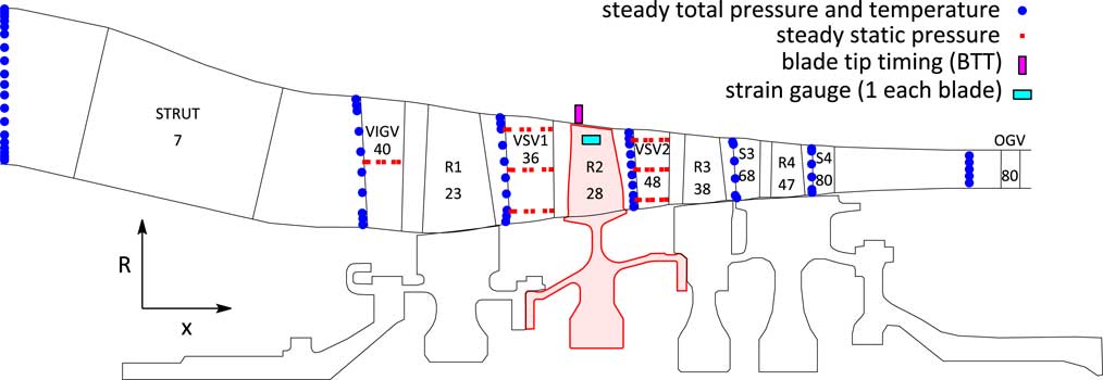
This paper is a sequel of the work of Schrape et al.( Reference Schrape, Giersch, Nipkau, Stapelfeldt and Mück 9 ) and aims at drawing a more complete picture of the impact of TSMs on forced vibration responses by adding more theoretical aspects and comparing predicted with measured rig data. Subject of interest is a 4.5-stage research axial compressor rig located at the German Aerospace Center (DLR) in Cologne, see Fig. 6 for a general arrangement of the rig with the most relevant instrumentation and blade counts. Within the recent build the second rotor stage has been replaced by a blisk design, that is instrumented with strain gauges on every blade. Additionally, blade tip timing (BTT) is installed. Both measurement systems allow to monitor each blade response individually.
During the preparation of the test campaign several mistuning measurements of different configurations (single blisk stage before and after instrumentation as well as the assembled rotor drum) have been carried out( Reference Beirow, Kühhorn, Figaschewsky, Hönisch, Giersch and Schrape 12 ). The used aeromechanical ROM, a subset of nominal system modes (SNMs) representation( Reference Yang and Griffin 6 ), is able to take into account mistuning effects, aerodynamic damping and gyroscopic loads. The model has been validated for the particular rotor and studied mode family with the obtained vibration measurements at rest by comparing predicted and identified mistuned mode shape envelopes. Details of the mistuning measurement campaign and the validation process can be found in Ref. Reference Beirow, Kühhorn, Figaschewsky, Hönisch, Giersch and Schrape12.
Such a ROM is traditionally used to study the effect of mistuning on the forced vibration behaviour due to a single engine order excitation acting on a single travelling wave mode (TWM)( Reference Whitehead 2 , Reference Giersch, Hönisch, Beirow and Kühhorn 7 , Reference Besem, Kielb and Key 13 , Reference Figaschewsky, Kühhorn, Beirow, Nipkau, Giersch and Power 14 ). The derived frequency response functions (FRFs) and blade individual vibration amplitudes can then be compared with those obtained in measurements – sometimes with unsatisfying agreement on some of the blades and unexpected nodal diameter content in the response( Reference Besem, Kielb and Key 13 ). This might be due to the simplification of the force vector by restricting it to act on a single nodal diameter which does not hold in general – especially in a multistage engine.
1.1 Unsteady pressure field in multistage environment
Before the influence of multiple TWMs appearing on the right-hand side of the equations of motions is studied, this section is meant to visualise the physics involved in the generation of TSMs as well as their consequence in terms of blade individual excitation force. Therefore, this study regards a stationary blade row with N S vanes and a rotating blade row with N R blades in undistorted inlet flow conditions. Both bladerows are assumed to have a perfect cyclic periodicity i.e. all blades of each bladerow have identical geometry. Consequently, each quantity of the flow field is not only periodic with respect to a complete revolution but also with respect to a single blade passage due to the wall boundary condition on the blade’s surfaces. Thus, the pressure field can be expanded in a Fourier series with amplitude c k and phase γ k of the distinct harmonic components kN S or lN R , respectively, each in its frame of reference. Let φ′ be the circumferential co-ordinate in the rotating frame of reference and φ=φ′ + Ωt the circumferential coordinate in the stationary frame of reference with Ω being the shaft speed of the rotor. The pressure field p S (φ′, t) (stator) or p R (φ′) (rotor) for each location and bladerow regarded separately then reads in the rotating frame of reference:
 $$p_{S} ({\rm \rvarphi '},t){\equals}\mathop{\sum}\limits_{k{\equals}0}^\infty c_{{S,k}} \cos (kN_{S} ({\rm \rvarphi '}{\plus}\Omega t){\minus}{\rm \gamma }_{{S,k}} )$$
 $$p_{R} ({\rm \rvarphi '}){\equals}\mathop{\sum}\limits_{l{\equals}0}^\infty c_{{R,l}} \cos (lN_{{ R}} {\rm \rvarphi '}{\minus}{\rm \gamma }_{{{ R},l}} )$$
In between the two regarded bladerows, there is an interaction zone, where the flow field has to satisfy both wall boundary conditions at the same time. The most comprehensible expansion of the solution is the product of the two Fourier series above:
 $$p({\rm \rvarphi '},t){\equals}p_{S} ({\rm \rvarphi '},t) \cdot p_{R} ({\rm \rvarphi '}){\equals}\mathop{\sum}\limits_{k{\equals}0}^\infty p_{k} ({\rm \rvarphi '},t)$$
The unsteady pressure in the rotating frame of reference is composed of multiple harmonics p k (φ′,t) of the number of stator vanes with the following definition:
 $$\hskip -0pt p_{k} ({\rm \rvarphi '},t){\equals}c_{{S,k}} \cos \left[ {kN_{S} ({\rm \rvarphi '}{\plus}\Omega t){\minus}\gamma _{{S,k}} } \right]\mathop{\sum}\limits_{l{\equals}0}^\infty c_{{R,l}} \cos (lN_{R} {\rm \rvarphi '}{\minus}{\rm \gamma }_{{R,l}} )$$
 $$\eqalignno { \hskip 28pt {\equals}a_{k} ({\rm \rvarphi '})\cos (kN_{S} \Omega t){\minus}b_{k} ({\rm \rvarphi '})\sin (kN_{S} \Omega t)\quad {\rm with\,\colon\,} \cr \hskip 3pt a_{k} ({\rm \rvarphi '}){\equals}c_{{S,k}} \cos [kN_{S} {\rm \rvarphi '}{\minus}\gamma _{{S,k}} ]\mathop{\sum}\limits_{l{\equals}0}^\infty c_{{R,l}} \cos (lN_{{ R}} {\rm \rvarphi '}{\minus}{\rm \gamma }_{{{ R},l}} )\quad {\rm and} \cr \hskip 3ptb_{k} ({\rm \rvarphi '}){\equals}c_{{S,k}} \sin [kN_{S} {\rm \rvarphi '}{\minus}\gamma _{{S,k}} ]\mathop{\sum}\limits_{l{\equals}0}^\infty c_{{R,l}} \cos (lN_{{ R}} {\rm \rvarphi '}{\minus}{\rm \gamma }_{{{ R},l}} ) $$
The unsteady pressure field contains products of the form
 $$\cos (kN_{S} {\rm \rvarphi '})\cos (lN_{R} {\rm \rvarphi '})$$
that translate into spatially harmonic functions of the form
$$\cos (kN_{S} {\rm \rvarphi '})\cos (lN_{R} {\rm \rvarphi '})$$
that translate into spatially harmonic functions of the form
 $$\cos \left[ {(kN_{S} {\plus}lN_{R} ){\rm \rvarphi '}} \right]$$
and
$$\cos \left[ {(kN_{S} {\plus}lN_{R} ){\rm \rvarphi '}} \right]$$
and
 $$\cos \left[ {(kN_{S} {\minus}lN_{R} ){\rm \rvarphi '}} \right]$$
. After some rearrangements of Equation (5), the unsteady pressure field in the rotating frame of reference reads:
$$\cos \left[ {(kN_{S} {\minus}lN_{R} ){\rm \rvarphi '}} \right]$$
. After some rearrangements of Equation (5), the unsteady pressure field in the rotating frame of reference reads:
 $$p({\rm \rvarphi '},t){\equals}\mathop{\sum}\limits_{k{\equals}0}^\infty p_{k} ({\rm \rvarphi '},t){\equals}\mathop{\sum}\limits_{k{\equals}0}^\infty \mathop{\sum}\limits_{l{\equals}{\minus}\infty}^\infty C_{{kl}} \cos \left[ {(kN_{S} {\plus}lN_{R} ){\rm \rvarphi '}{\plus}kN_{S} \Omega t{\minus}{\rm \rpsi }_{{kl}} } \right]$$
Equation (6) shows that the unsteady pressure field in the rotating frame of reference consists of multiple travelling waves with nodal diameter kN
S
+ lN
R
, that are referred to the TSMs. The focus is now shifted on the effect of such a pressure field generated by a rotor–stator interaction acting on another rotor with N blades upstream or downstream of the generating bladerows. Therefore, the amplitude of the unsteady pressure component
 $$\hat{p}_{k} ({\rm \rvarphi '})$$
is studied:
$$\hat{p}_{k} ({\rm \rvarphi '})$$
is studied:
 $$\hat{p}_{k} ({\rm \rvarphi '}){\equals}\sqrt {a_{k}^{2} ({\rm \rvarphi '}){\plus}b_{k}^{2} ({\rm \rvarphi '})} {\equals}\mathop{\sum}\limits_{l{\equals}0}^\infty 2C_{{kl}} \cos (lN_{{ R}} {\rm \rvarphi '}{\minus}{\rm \gamma }_{{R,l}} )$$
Evaluating Equation (7) for φ′=2πj/N, it can be noticed that not only the mean value but also the amplitude of the unsteady pressure – and hence the modal force in the engine order kN S – is a function of the blade number j. Thus, every blade of the target rotor faces an individual amplitude of the modal force inherently leading to blade individual vibration amplitudes, even in the absence of mistuning. However, this only holds if the interaction zone of the generating blade row extends to the upstream or downstream rotor and the number of blades N R of the source rotor is no integer multiple of the number of blades N of the affected rotor. Whenever either of the cases above is not satisfied, the modal force on each of the blades will be constant i.e. the TSMs generated by a rotor itself do not lead to blade individual modal forces. It needs a second rotating blade row for this effect to occur, and thus, the influence of TSMs on forced response does only affect multistage engines.
The differences in the blade individual excitation depend on the clocking of the two rotating bladerows and on the amplitude of the harmonic components generated by the source rotor. Thus, there have to be any flow features e.g. cut-on pressure waves, strong wakes, shocks, or separations, that are able to interact with the flow field of the stator responsible for the excitation.
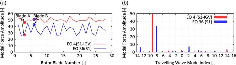
To illustrate the physics involved in such an interaction, a quasi 2D simulation of the front stages (IGV to Rotor 3) of the regarded compressor rig (see Fig. 6 for blade counts and an illustration) has been carried out. Therefore, a section at 85% span has been extracted, since this is assumed to be most representative for the excitation of modes with its maximum in the tip region. Figure 1 shows instantaneous entropy contours of four snapshots of the unsteady simulation. Each snapshot is taken when the highlighted blades A and B are about to hit the wake of the upstream stator. The depicted domain extends from Rotor 1 (top bladerow) to Rotor 2 (bottom bladerow). The operating condition is at part-speed with malscheduled VSVs responsible for the low incidence on the Stator 1 and a flow separation on its pressure side. This flow separation is sensitive to the wake of the upstream rotor, such that the separation becomes coherent with respect to the blade passing. The strength of the stator’s wake becomes a harmonic function of time with its frequency modulated by the upstream rotor. Thus, the excitation faced by the downstream Rotor 2 will depend on the clocking with respect to the Rotor 1. This can be visualised by tracking the two highlighted blades A and B in Fig. 1. Whereas blade A always hits a weak wake, blade B is exposed to a much stronger wake due to the interaction of the wake with the upstream rotor. To quantify the effect on the forced response, a mode shape similar to the 3D mode shape depicted in Fig. 11 is studied for a section at 85% span. The effect on the modal force of blades A and B is shown in Fig. 2. The modal force difference observed when hitting the upstream stator’s wake is significantly stronger on blade B and as a consequence the excitation in the EO36 (upstream Stator 1) on blade B is 55% higher than on blade A. The overall pattern of the blade individual excitation force in the most dominant frequencies – EO4 (difference of upstream IGV and S1) and EO36 (upstream S1) – is depicted in Fig. 3(a).
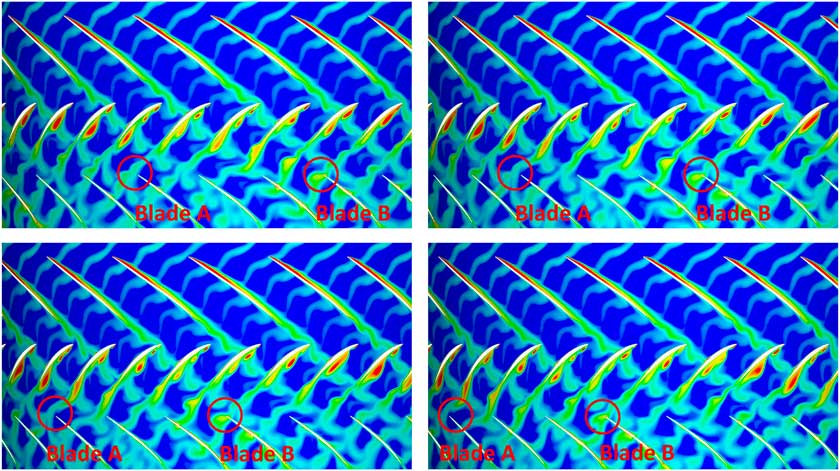
Figure 1 Entropy contours (blue = low, red = high) of snapshots of an unsteady Q2D simulation taken when R2 hit the VSV1 wake 4 consecutive times.
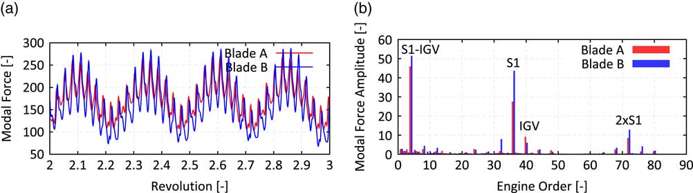
Figure 2 Time history of modal force vs revolution (a) and frequency content of modal force (b) for blades A and B.

Figure 3 Modal force amplitudes of the most dominant engine orders 4 and 36 vs Rotor 2 blade number (a) and traveling wave mode index (b).
1.2 Effect on forced response
This section studies the influence of TSMs on the forced response of a real rotor. Since the blades are structurally coupled, the knowledge of the blade individual force is not enough to predict the induced amplification of the vibration amplitude. Therefore, the spatial harmonic content of the excitation needs to be analysed. The excitation contains spatial modes with nodal diameters k=N S ± lN R with N R and N S being the blade counts of the generating rotor and stator. To identify the corresponding aliased TWM in the affected rotor domain with N blades and maximum nodal diameter k max=N/2 (N even) or k max=(N−1)/2 (N odd), the following formula needs to be evaluated for k=N S ± lN R :
 $$k_{{{\rm alias}}} (k){\equals}(k_{{{\rm max}}} {\minus}k)\,{\rm mod}\,N{\minus}k_{{{\rm max}}} {\equals}(k_{{{\rm max}}} {\minus}(N_{S} \,\pm\,lN_{R} ))\,{\rm mod}\,N{\minus}k_{{{\rm max}}} $$
 $$\hskip 20pt\,\equiv\,(k_{{{\rm max}}} {\minus}(N_{S} \,\mp\,l\Delta N))\,{\rm mod}\,N{\minus}k_{{{\rm max}}} \quad {\rm with}\,\Delta N{\equals}N_{R} {\minus}N$$
A negative sign implies a backward TWM and a positive sign a forward TWM with respect to the rotating frame of reference. It has been already discussed that the self-influence of the TSM of one rotor–stator interaction does not lead to blade individual force amplitudes. The formula above also shows that for N R =N all these components alias on the same TWM k alias(N S ), and thus, the effect of TSMs on forced response is only present in multi-stage engines.
Evaluating the formula above for the studied configuration with N S =36, N R =23, and N=28, the aliased TWMs of the first seven TSMs are −8, −13, −3, 10, 2, 5, 7 for l=0, 1, −1, 2, −2, 3, −3, respectively. The presence of these excitations is also proved with the quasi 2D simulation. A decomposition of the modal force into TWMs is shown in Fig. 3(b) with present TSM components, especially in the TWMs −13 and 2. It is also worth to mention that the excitation in the EO4 acts on the TWM −9, which is the aliased TWM for N S =4 and l=1 i.e. the first TSM for the EO4 excitation.
To understand the effect on blade individual vibration amplitudes, the modal transformed equations of motions for a tuned rotor are studied in a TWM basis:
 $${\bf x}(t){\equals}\Re \left\{ {\mathop{\sum}\limits_{m{\equals}1}^{N_{{{\rm modes}}} } \underline{q} _{m} \underline{\Phi } _{m} {\rm e}^{{i(\Omega _{{N_{S} }} t{\minus}k_{m} \rvarphi ')}} } \right\}$$
Each of the modes with modeshape vector
 $$\underline{\Phi } _{m} $$
and modal amplitude
$$\underline{\Phi } _{m} $$
and modal amplitude
 $$\underline{q} _{m} $$
has a certain natural frequency ω
m
, damping δ
m
and nodal diameter k
m
. For the sake of clarity, only one additional TWM component is regarded besides the nominal one and a blade dominated mode family is assumed with N
modes=N modes and identical mode shape vectors
$$\underline{q} _{m} $$
has a certain natural frequency ω
m
, damping δ
m
and nodal diameter k
m
. For the sake of clarity, only one additional TWM component is regarded besides the nominal one and a blade dominated mode family is assumed with N
modes=N modes and identical mode shape vectors
 $$\Phi _{m} $$
with maximum deflection
$$\Phi _{m} $$
with maximum deflection
 $$\hat{\Phi }$$
. The upgraded right-hand side f(t) contains TWM excitation forces of the form:
$$\hat{\Phi }$$
. The upgraded right-hand side f(t) contains TWM excitation forces of the form:
 $$f(t){\equals}\Re \left\{ {\underline{{\hat{f}}} {\rm e}^{{i(\Omega _{{N_{S} }} t{\minus}k\rvarphi ')}} } \right\}$$
with two different nodal diameters k
1=k
alias(N
S
) and k
2=k
alias(N
S
+ lΔN) acting in the same excitation frequency
 $$\Omega _{{N_{S} }} {\equals}N_{S} \Omega $$
. The modal equations of motion read
$$\Omega _{{N_{S} }} {\equals}N_{S} \Omega $$
. The modal equations of motion read
 $${\rm diag}\left\{ {{\rm \romega }_{m}^{2} {\minus}\Omega _{{N_{S} }}^{2} {\plus}2i\Omega _{{N_{S} }} {\rm \rdelta }_{m} } \right\}\underline{{\bf q}} {\equals}\underline{{\bf f}} {\equals}\left[ {\matrix{ {0\,\ldots\,0} & {\underline{\hat f} _{1} } & {0\,\ldots\,0} & {\underline{\hat f} _{2} } & {0\,\ldots\,0} \cr } } \right]^{T} $$
The vibrational response
 $$x_{j}^{0} (t)$$
for the point with the maximum mode deflection
$$x_{j}^{0} (t)$$
for the point with the maximum mode deflection
 $$\hat{\Phi }$$
obtained at
$$\hat{\Phi }$$
obtained at
 $$\Omega _{{N_{S} }} {\equals}\romega _{1} $$
with the classical excitation vector without additional TSM components is given by a travelling wave with constant amplitude for each of the blades:
$$\Omega _{{N_{S} }} {\equals}\romega _{1} $$
with the classical excitation vector without additional TSM components is given by a travelling wave with constant amplitude for each of the blades:
 $$x_{j}^{0} (t){\equals}\Re \left\{ {{{\underline{\hat f} _{1} {\rm e}^{{{\minus}ik_{1} {\rm \rvarphi' }_{{j}} }} } \over {2iD_{1} {\rm \romega }_{1}^{2} }}\hat{\Phi }{\rm e}^{{i{\rm \romega }_{1} t}} } \right\}{\equals}\Re \left\{ {\underline{\hat x} _{j}^{0} {\rm e}^{{i{\rm \romega }_{1} t}} } \right\}{\rm with}\,{\rm \rvarphi '}_{{j}} {\equals}{{2{\rm \pi }j} \over N}$$
Considering the additional TSM component, the blade individual vibration amplitude of the jth blade of the tuned system is given by the superposition of the two tuned modes with nodal diameter k 1 and k 2:
 $$x_{j} (t){\equals}\Re \left\{ {\left[ {{{\underline{{\hat{f}}} _{1} {\rm e}^{{{\minus}ik_{1} {\rm \rvarphi '}_{j} }} } \over {{\rm \romega }_{1}^{2} {\minus}\Omega _{{N_{S} }}^{2} {\plus}2i\Omega _{{N_{S} }} {\rm \rdelta }_{1} }}{\plus}{{\underline{{\hat{f}}} _{2} {\rm e}^{{{\minus}ik_{2} {\rm \rvarphi '}_{j} }} } \over {{\rm \romega }_{2}^{2} {\minus}\Omega _{{N_{S} }}^{2} {\plus}2i\Omega _{{N_{S} }} {\rm \rdelta }_{2} }}} \right]\hat{\Phi }{\rm e}^{{i\Omega _{{N_{S} }} t}} } \right\}{\equals}\Re \left\{ {\underline{{\hat{x}}} _{j} (\Omega _{{N_{S} }} ){\rm e}^{{i\Omega _{{N_{S} }} t}} } \right\}$$
Normalising Equation (14) with the blade individual response
 $$\underline{{\hat{x}}} _{j}^{0} $$
obtained from the classical right hand side at
$$\underline{{\hat{x}}} _{j}^{0} $$
obtained from the classical right hand side at
 $$\Omega _{{N_{S} }} {\equals}{\rm \romega }_{{\rm 1}} $$
(Equation (13)) yields the relative change in the vibration response
$$\Omega _{{N_{S} }} {\equals}{\rm \romega }_{{\rm 1}} $$
(Equation (13)) yields the relative change in the vibration response
 $$\underline{{{\rm \eta }_{j} }} $$
:
$$\underline{{{\rm \eta }_{j} }} $$
:
 $$\underline{{\rm \eta }} _{j} {\equals}{{\underline{{\hat{x}}} _{j} {\minus}\underline{{\hat{x}}} _{j}^{0} } \over {\underline{{\hat{x}}} _{j}^{0} }}{\equals}{{\underline{{\hat{f}}} _{2} } \over {\underline{{\hat{f}}} _{1} }}{{D_{1} } \over {D_{2} }}{1 \over {(r^{2} {\minus}1)\,/\,2iD_{2} {\plus}r}}{\rm e}^{{{\minus}i(k_{2} {\minus}k_{1} ){\rm \rvarphi '}_{{j}} }} \quad {\rm with}\,D_{m} {\equals}{\rm \rdelta }_{m} \,/\,{\rm \romega }_{m} {\rm ,}\ r{\equals}{\rm \romega }_{2} \,/\,{\rm \romega }_{1} $$
The blade individual deviation of the vibration response is not only a function of the force ratio
 $$r_{f} {\equals}\underline{\hat f} _{2} \,/\,\underline{\hat f} _{1} $$
but also a function of the damping ratio D
2/D
1 as well as the amount of the frequency distance r of the two system modes in relation to the damping D
2. Furthermore, Equation (15) reveals that the blade individual vibration amplitude is a harmonic function with wave number k
2−k
1=lΔN. Introducing the relative frequency spread
$$r_{f} {\equals}\underline{\hat f} _{2} \,/\,\underline{\hat f} _{1} $$
but also a function of the damping ratio D
2/D
1 as well as the amount of the frequency distance r of the two system modes in relation to the damping D
2. Furthermore, Equation (15) reveals that the blade individual vibration amplitude is a harmonic function with wave number k
2−k
1=lΔN. Introducing the relative frequency spread
 $${\rm \rho }{\equals}\!\mid\!\!({\rm \romega }_{2} {\minus}{\rm \romega }_{1} )\!\!\mid\!\!/{\rm \romega }_{1} {\equals}\!\mid\!\!r{\minus}1\!\!\mid\!$$
and assuming a constant and sufficiently small ratio of critical damping D
1=D
2=D≪1, Equation (15) can be simplified to calculate the maximum possible relative increase
$${\rm \rho }{\equals}\!\mid\!\!({\rm \romega }_{2} {\minus}{\rm \romega }_{1} )\!\!\mid\!\!/{\rm \romega }_{1} {\equals}\!\mid\!\!r{\minus}1\!\!\mid\!$$
and assuming a constant and sufficiently small ratio of critical damping D
1=D
2=D≪1, Equation (15) can be simplified to calculate the maximum possible relative increase
 $${\rm \hat{\eta }}_{j} $$
of the vibration amplitude due to one additional TSM component:
$${\rm \hat{\eta }}_{j} $$
of the vibration amplitude due to one additional TSM component:
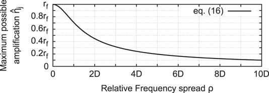
 $${\rm \hat{\eta }}_{j} {\equals}r_{f} {{\sqrt {1{\plus}({\rm \rho }\,/\,D)^{2} } } \over {1{\plus}({\rm \rho }\,/\,D)^{2} }}$$
Figure 4 shows the suppression of the amplification as a function of the relative frequency spread ρ and damping level D 1=D 2=D.

Figure 4 Maximum possible amplification as a function of force ratio r f , damping level D 1=D 2=D≪1 and relative frequency spread ρ.
Thus, the occurrence of additional TSM components in the excitation i.e. blade individual force amplitudes, does not necessarily lead to a significant amplification of the vibrational response. The system modes need to be close enough to make the TSMs affect the vibration amplitudes significantly. The worst case would be to excite a very close system mode (ρ ≈ 0) with lower damping (D 2 ≪ D 1). On the other hand, the amplification is suppressed, if the system modes are sufficiently far spread i.e. ρ ≫ D. In such a case, one would observe two distinct peaks in the FRF without any influence of one onto the other.
Figure 5 shows the effect of the first two TSMs for l=−1 (left column) and l=1 (right column) on a tuned example configuration of the Rotor 2 (N=28) affected by the TSMs generated by Rotor 1 (N
R
=23) acting in the excitation frequency of the VSV1 (N
S
=36). According to Equation (9), the nominally excited TWM would be TWM −8. For l=−1, a forcing of the TWM −3 is introduced and for l=1 a forcing of the TWM −13 is introduced. Figures 5a and b show the natural frequency vs TWM index of the example configuration with the excited TWM components highlighted. While TWM −13 is very close to TWM −8 (ρ=0.018%=1.8D), TWM −3 has a large distance (ρ=0.2%=20D) compared to the chosen damping level of 0.01%. The effect on the forced response is visualised by the FRFs in Figs 5(c) and 5(d). Whereas a significant interaction of the two TWMs can be observed for the close system modes (see Fig. 5(d)), there is almost no influence of the additional TWM component on the nominal response in case of sufficiently far spread system frequencies (ρ ≫ D, see Fig. 5c). According to Equation (4), the amplification of individual vibration levels is much higher (
 $$\hat{\eta }_{j} (1.8D)\,\approx\,0.5r_{f} \,\approx\,0.2$$
) in Fig. 5f and almost suppressed in the other case (
$$\hat{\eta }_{j} (1.8D)\,\approx\,0.5r_{f} \,\approx\,0.2$$
) in Fig. 5f and almost suppressed in the other case (
 $${\rm \hat{\eta }}_{j} (20D)\,\approx\,0.05r_{f} \,\approx\,0.02$$
, see Fig. 5e. Both cases confirm the theoretical prediction of the harmonic pattern with wave number ΔN=5 (compare Equation (15)).
$${\rm \hat{\eta }}_{j} (20D)\,\approx\,0.05r_{f} \,\approx\,0.02$$
, see Fig. 5e. Both cases confirm the theoretical prediction of the harmonic pattern with wave number ΔN=5 (compare Equation (15)).
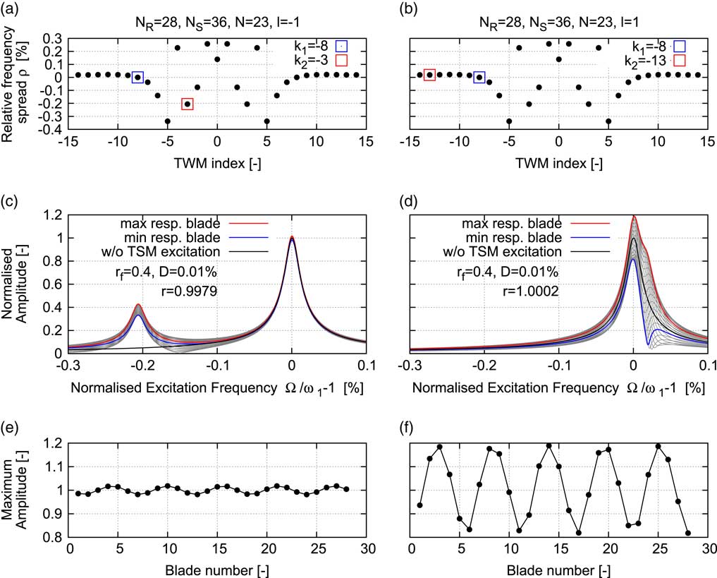
Figure 5 Natural frequency vs TWM index (a and b), blade individual FRFs (c and d), and maximum vibration amplitude (e and f) for a tuned example configuration with one additional TSM excitation component: l = −1 (left column: a, c, and e) and l = 1 (right column: b, d, and f).
It can be concluded that it needs to have a multistage engine with both a sufficiently strong presence of the interaction modes and a region of high modal density i.e. small frequency deviations of the system modes, for the forced response to be affected by TSMs.
2.0 COMPRESSOR RIG TEST CASE
This section shifts the focus from the theoretical studies to a real test case. Subject of the investigations is the Rotor 2 blisk stage of an axial high pressure compressor rig with 4.5 stages, see e.g. Refs Reference Schrape, Giersch, Nipkau, Stapelfeldt and Mück9, Reference Johann, Mueck and Nipkau15, Reference Roeber, Kuegeler and Weber16 for a more detailed description of the facility. A general arrangement of the rig with the instrumentation being most important for this study is sketched in Fig. 6. The leading edges of some of the vanes of each stator row are instrumented with steady total pressure and total temperature probes and some of the variable vanes have steady static pressure probes on sections of the blade profile. These measurement systems are able to track the steady state performance of the entire rig as well as of single blocks. Also, they allow for a validation of the steady state CFD solutions close to the resonance speed of interest. The focus is on the highlighted Rotor 2 blisk, which is instrumented with one strain gauge per blade. Additionally, BTT is installed. Both measurement systems allow to monitor the vibration response of each blade individually which makes this rotor of the compressor rig a perfect specimen to study the effect of TSMs on the forced response.

Figure 6 Sketch and blade counts of the investigated compressor rig with the most important instrumentation and the idealised shaft geometry with highlighted Rotor 2 blisk.
2.1 Investigated resonance condition
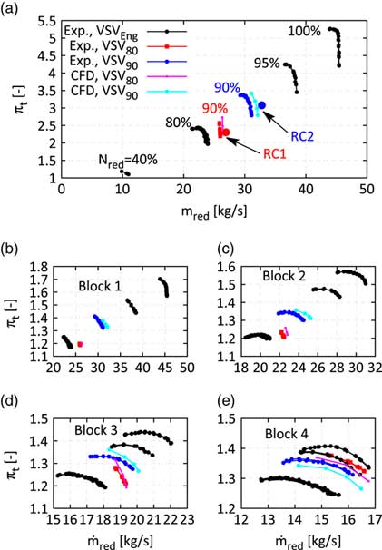
Figure 8 shows the Campbell diagram of the studied Rotor 2 blisk with the most dominant upstream excitation sources. Focus of this investigation will be on the mode 11 (M11) resonance with engine order 36 (EO36) at approximately 91% mechanical speed. The compressor rig features three variable stator vanes (VSVs) which are adjusted stepwise at predefined reduced speeds. Depending on the inlet temperature, the resonance is very close to a point where the VSVs are shifted, such that the rig has been operated with a constant VSV schedule for the studied forced response experiments. The identical mechanical resonance has been crossed with two different constant VSV schedules, the schedules of 80% and 90% reduced speed, respectively. The first one will be referred to VSV80 the latter one to VSV90. The application of two different VSV schedules shifts the occurrence of the mechanical resonance in the compressor map, see Fig. 7a. Both resonance conditions RC1 (with VSV80) and RC2 (with VSV90) are studied on a low working line, see the position of the points with respect to the characteristics obtained at 90% reduced speed with the respective schedule. Figures 7b and e show the blockwise performance (Block 1: Inlet-VSV1, Block 2: VSV1-VSV2, Block 3: VSV2-S3, Block 4: S3-OGV) of the compressor and reveal a significant change of the nature of the flow in the front rotors (R1 and R2) when the VSV80 schedule is applied at 90% speed. Hence, it implies a noticeable impact on the strength of the generated TSMs.
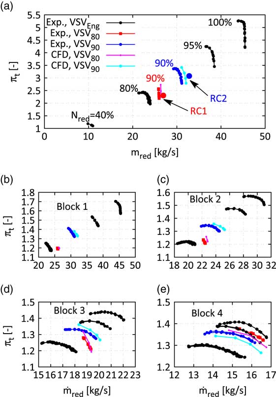
Figure 7 Measured compressor map of the whole rig (a) and single blocks (b–e) with the two distinct mode 11 resonance conditions RC1 and RC2.
Omitting the effect of TSMs on the forced response the vibration amplitude vs blade pattern as well as the FRFs for the two different resonance conditions should only differ by a scaling factor as long as the aerodynamic damping does not change too significantly. Hence, any change in the amplitude vs blade pattern and in the shape of the FRFs will be dedicated to the influence of the present TSMs i.e. by comparing the two resonance conditions, it can be directly assessed whether TSMs are able to affect the forced response and to which extent they do. The measured results are compared with analytical predictions that are introduced in the following sections.
2.2 Structural model
This section describes the structural model used for the assessment of the mistuned vibration behaviour of the Rotor 2 blisk with TSM excitation on the right-hand side. The assessment is done with a ROM based on a SNM approach( Reference Yang and Griffin 6 ). The SNM uses 32 nominal system modes in the frequency range of mode 11 that are derived from a finite element (FE) model of the Rotor 2 blisk. However, the boundary conditions at the front and rear flange are difficult to choose. Clamped boundary conditions might suppress disk modes, free boundary conditions might be too soft generating artificial disk modes. Regardless of the presence of any disk modes, the structural coupling of the blades via the disk has to be modelled most realistic in order to calculate the natural frequencies of the tuned system modes of the studied mode family as accurate as possible since it turned out that the influence of TSMs (see Equation (15)) as well as the influence of mistuning heavily depends on the nodal diameter vs frequency map (Fig. 8).
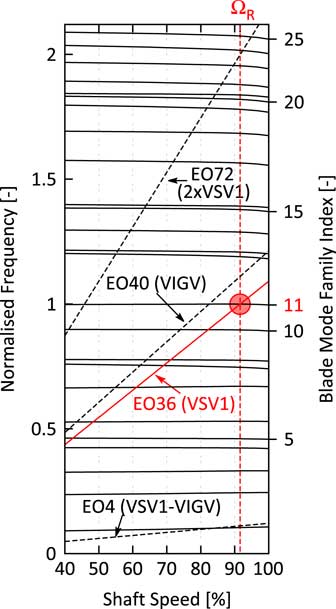
Figure 8 Campbell diagram of the studied rotor.
Therefore, an idealised geometry of the assembled shaft has been generated and merged with the Rotor 2 blisk stage. Finally, a sector model of the whole assembly is derived, see Figs 6 and 9. Since the extracted sector is not correlated to the other rotor blade counts (R1, R3 and R4), they cannot be included with their real geometry. Their influence on the static deflection of the whole shaft is taken into account by adding a thin layer of surrogate elements on the respective surface where the blades would be attached to their disks. The surrogate elements of each rotor stage get an artificial density to match the mass of all blades of this rotor stage divided by the number of Rotor 2 blades. Thus, an appropriate centrifugal load acts on the R1, R3 and R4 disks. By the application of this, surrogate mass also the inertial force of the blades is taken into account in the modal analysis step. The whole shaft is treated as one integral part and boundary conditions are applied at the approximate position of the bearings. By this procedure, the effect of artificial boundary conditions at the flanges is removed, whereas the uncertainty due to the simplification of the disk contacts remains. This simplification is necessary as long as a linear theory is regarded. The blade mode shape of mode family 11 is shown in Fig. 11a. Based on the computed system modes, the SNM representation of the rotor can be built. The used implementation of the SNM is able to take into account the effect of mistuning, aerodynamic damping, and Coriolis loads, see( Reference Yang and Griffin 6 , Reference Giersch, Hönisch, Beirow and Kühhorn 7 , Reference Figaschewsky, Kühhorn, Beirow, Nipkau, Giersch and Power 14 ) for a more detailed description of the SNM implementation. Several mistuning measurements of the Rotor 2 blisk are available (before and after instrumentation as well as after assembling of the drum), see( Reference Beirow, Kühhorn, Figaschewsky, Hönisch, Giersch and Schrape 12 ) for a detailed description of the measurement campaign and Fig. 10 for the mistuning pattern obtained after the assembling of the drum. Also, the SNM approach for the studied mode family has been at least validated at rest by the means of a comparison of predicted mistuned mode shape envelopes with measured ones, see also( Reference Beirow, Kühhorn, Figaschewsky, Hönisch, Giersch and Schrape 12 ).
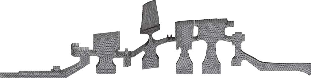
Figure 9 Finite element model of the rotor.
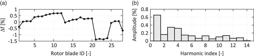
Figure 10 Identified frequency mistuning pattern for the studied blade mode family 11( Reference Beirow, Kühhorn, Figaschewsky, Hönisch, Giersch and Schrape 12 ) (a) and the harmonic amplitudes of its discrete fourier transform (b).
The computed nodal diameter vs frequency map is depicted in Fig. 11b. It also shows the influence of the gyroscopic loads (Coriolis terms) on the split of the tuned double modes. Especially, the low nodal diameter modes are subject to a noticeable shift of the backward and forward TWMs. Finally, the influence of the measured mistuning pattern is added leading to the prediction of a significant spread of the natural frequencies. Figure 11c compares the position of the mistuned natural frequencies with the envelope of the measured mode 11 response of all strain gauges. It can be noticed that the overall width of the resonance is correctly captured by the model even though the measured frequency spread due to mistuning is slightly higher. Thus, the structural model is assumed to be suitable for the prediction of the influence of TSMs on the mistuned forced response of the studied mode family 11. The resonance features multiple dominant peaks i.e. the ratio of the damping is rather low compared to the frequency distance of the system modes and the effect of blade individual forces cannot be directly translated into differences of maximum vibration amplitudes, compare Equation (15) and its interpretation above. Consequently, the combination of TSMs and mistuning will lead to complex interactions in the FRFs that will be assessed by the ROM.
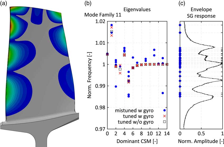
Figure 11 Studied blade mode 11: mode shape (a), eigenvalues vs dominant cyclic symmetry mode for different structural models (b) and envelope of the measured mode 11 SG response vs frequency (c).
2.3 Flow model
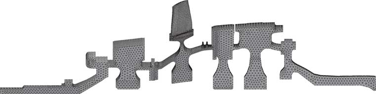
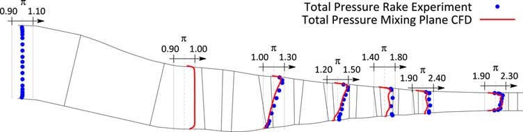
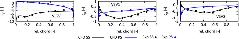
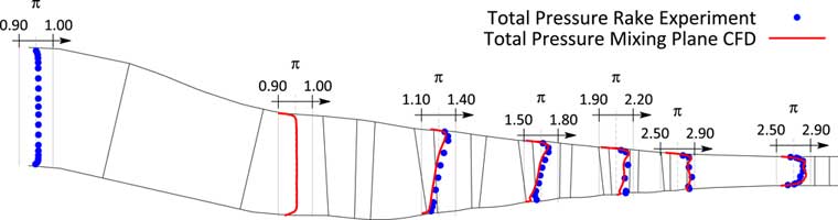
In order to assess the strength of TSMs at a certain operating condition, unsteady simulations of large CFD models have to be run. Since these simulations are based on respective steady state simulations, the focus of this section is on the validation of the flow model by comparing the predicted with the measured steady state performance. Therefore, a single passage model of the compressor consisting of 11 bladerows from the strut to the outlet guide vane is built. The bladerows are connected via mixing planes. The used nonlinear flow solver has been developed by the Imperial College in London( Reference Sayma, Vahdati and Imregun 17 , Reference Vahdati, Sayma and Imregun 18 ). The used meshes are semiunstructured i.e. structured in the spanwise direction but each layer contains an unstructured mesh, compare( Reference Sbardella, Sayma and Imregun 19 , Reference Stelldinger, Giersch, Figaschewsky and Kühhorn 20 ) for a more detailed description of the meshing philosophy. Fillets and varying gap sizes are taken into account, compare also( Reference Schrape, Giersch, Nipkau, Stapelfeldt and Mück 9 , Reference Stelldinger, Giersch, Figaschewsky and Kühhorn 20 ). Measured radial total pressure and total temperature profiles are applied at the inlet of the domain and a choked nozzle with variable area is attached to the outlet of the domain to adjust the working line of the compressor. For the reason of clarity, Fig. 7 compares only the characteristics at 90% reduced speed predicted by the CFD for the 80% and 90% VSV schedule. It can be noticed that not only the overall performance agrees well with the measurement, but also the blockwise performance is very well reflected by the flow model. This impression is also confirmed by comparing measured radial total pressure profiles for the closest available steady-state scans for the two different schedules, see Figs 12 and 14. Finally, the measured and predicted pressure profiles, shown as pressure coefficient c p (c rel )=(p s (c rel )−p s,in )/(p t,in −p s,in ) as a function of the relative chord length c rel , on both suction and pressure side agree very well Figs 13 and 15.

Figure 12 Comparison of measured and simulated radial total pressure profiles for steady state scan closest to resonance condition RC1 (80% VSV schedule).

Figure 13 Comparison of measured and simulated blade static pressure profiles at 50% span for steady state scan closest to resonance condition RC1 (80% VSV schedule).
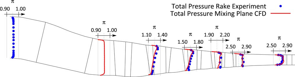
Figure 14 Comparison of measured and simulated radial total pressure profiles for steady-state scan closest to resonance condition RC2 (90% VSV schedule).
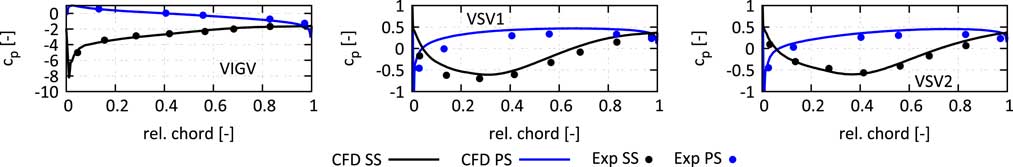
Figure 15 Comparison of measured and simulated blade static pressure profiles at 50% span for steady-state scan closest to resonance condition RC2 (90% VSV schedule).
All in all the flow model is in very good agreement with the measured steady-state performance and is assumed to be suitable for the following unsteady simulations.
2.4 Aerodynamic damping
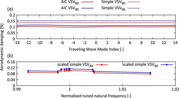
The mistuned forced response with or without TSM excitation is sensitive to the damping of the system. Since the regarded rotor is a blisk, aerodynamic damping is assumed to be the major source of damping present in the system. The method of aerodynamic influence coefficients is used to predict the aerodynamic damping. The flow model domain consists of five Rotor 2 blades, the initial flow solution and the boundary conditions at inlet and exit are extracted from a steady-state solution of the whole compressor model at resonance speed. 1D nonreflecting boundary conditions have been applied at the inlet and outlet of the domain and a single vibration cycle is resolved with 200 time steps. The single passage mode shape is derived from the nodal diameter 8 system mode shape, which is excited by the upstream stator if no TSMs are taken into account. Figure 16 shows the predicted aerodynamic damping as a function of the TWM index for both relevant schedules. The aerodynamic damping is almost a constant line indicating a vanishing influence of the adjacent blades i.e. the damping is dominated by the influence of the vibrating blade on itself and the influence of adjacent blades is negligible. Additionally, the vibration frequency is sufficiently high, such that the prerequisites of a simplified approach( Reference Figaschewsky, Kühhorn, Beirow, Giersch, Nipkau and Meinl 21 ), which is based on the radiation of sound waves to the far field, are satisfied and hence, it has also been applied. Whereas this simplified approach slightly overpredicts the aerodynamic damping (≈30%), it perfectly captures the relative increase of the aerodynamic damping of 25% from the VSV80 to the VSV90 schedule. Since some of the system modes present in the frequency range of the mode family 11 have a more or less pronounced disk motion, their aerodynamic damping will be affected simply due to the change of the modal mass of the mode. The simplified approach assesses these influences very efficiently. Hence, the output of the simplified approach is scaled, such that it matches the aerodynamic damping predicted by the unsteady CFD.
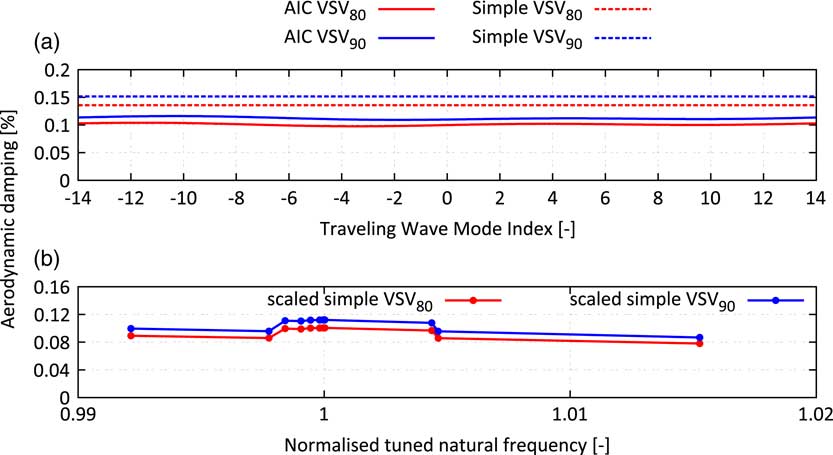
Figure 16 Aerodynamic damping computed with 3D CFD and predicted by simplified approach for ND8 mode shape (a) and scaled aerodynamic damping predicted by simplified approach vs tuned natural frequency of the applied system mode shape (b).
2.5 Aerodynamic excitation
In order to predict the strength of the TSMs for the different studied operating conditions, at least one of the adjacent rotors (R1 or R3) has to be present in the unsteady simulation. Therefore, a full circumference model of the front stages of the compressor rig is analysed. The largest CFD domain consists of eight bladerows being connected via sliding planes: Strut, VIGV, R1, VSV1, R2, VSV2, R3 and S3. This mesh has ≈70m nodes. The setup makes use of an unidirectional approach i.e. the blades do not vibrate in the assembly and the unsteady simulation does only monitor the aerodynamic excitation force on the rotor. The time step is chosen to resolve the blade passing of VSV1 and R2 (EO36) with 200 time steps which leads to 7,200 time steps per revolution. Unsteady pressure time histories of three shaft revolutions are recorded on every blade of the Rotor 2 which allows to assess the amplitude and phase information of the modal force for every system mode present in the ROM. It has been already mentioned that the amplitude vs blade patterns generated by TSMs depends on the clocking of the Rotor 2 with respect to the adjacent rotors. Thus, photographs taken during the mistuning measurement of the assembled drum have been analysed to estimate the relative position of a physical reference blade with respect to the Rotor 1. The evaluation of the modal force on the computational model is then shifted to account for the actual clocking situation in the real assembly.
A comparison of the largest setup (eight bladerows from Strut to S3) with a six bladerow setup (Strut to VSV2) showed no significant change of the forcing components i.e. in this particular case, the influence of the downstream rotor is negligible. Nevertheless, the following studies rely on the force predicted by the largest setup. Figure 17 shows the amplitude of calculated modal force as a function of the TWM index for both studied operating conditions normalised by the amplitude of the -8th TWM force. Thus, the amplitudes correspond to the force ratio r f introduced in the theory section in Equation (15). It can be noticed that for the VSV80 schedule, no significant amplification due to TSMs is expected with force ratios <0.15. Considering the tuned frequency distance of ND2 and ND8 of 0.1% and stacking up all the other TWM components, there remains an estimated deviation of ≈±20% which is assumed to be rather low compared to the amplification due to mistuning.
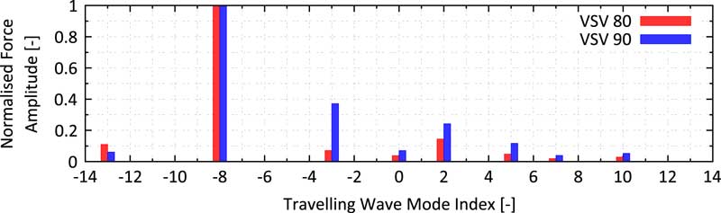
Figure 17 Normalised aerodynamic excitation predicted by the six blade row model as function of the TWM index for the two studied resonance conditions.
However, for the VSV90 schedule, there are a dominant −3 and +2 TWM force with force ratios of 0.38 and 0.25, respectively. Incorporating the tuned frequency split of 0.2% and 0.1%, an amplification of ≈±20% and ≈±17% can be estimated. Considering all the other components and a worst-case phasing of the TWMs, a local amplification up to 45% might be possible. In the most extreme case, a change in the VSV schedule might come along with a shift from +20% to −45% (or vice versa) on one of the blades and thus, a remarkable change in the amplitude vs blade pattern can be expected.
2.6 Vibration measurements
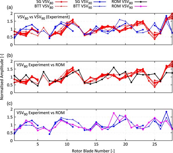
Figure 18a shows the measured amplitude vs blade patterns for the M11 EO36 resonance obtained from strain gauges (SGs, solid line) as well as with BTT (dashed line). The diagram contains six different curves for the VSV80 schedule derived from five accelerations with three different acceleration rates and one deceleration. Also, two different working lines have been tested, and the curves have been recorded on four different test days before and after the manoeuvre with the VSV90 schedule. All in all, it can be noticed that the measurement of the amplitude vs blade pattern is largely repeatable. Therefore, the patterns are assumed to be trustworthy in terms of measurement uncertainties despite the fact that for the VSV90 schedule only one forced response manoeuvre is available.
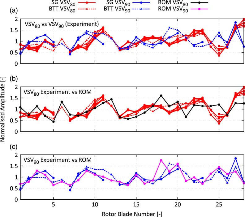
Figure 18 Blade individual vibration amplitudes: comparison of experiment at different resonance conditions (a); comparison of experiment and prediction for resonance condition 1 (b) and for resonance condition 2 (c).
In contrast to the largely repeatable curves for the VSV80 schedule, the second operating condition with VSV90 schedule produces a remarkably different amplitude vs blade pattern. Some of the blades increase or decrease their vibration amplitude with respect to the mean value significantly up to 100% (blade 25). Despite the increased aerodynamic damping level of +25%, that is able to change the coupling of the different TWMs, there is no other physical explanation leading to a different pattern than the presence of TSMs with sufficient strength. Thus, the change in the amplitude vs blade pattern proves the presence of TSMs in multistage engines and its effect on the forced response.
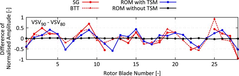
The increase of the strength of the TSM from the VSV80 to the VSV90 schedule has been already predicted by the CFD model. Also, the amplitude vs blade patterns predicted by the ROM show a reasonable agreement with the measurement (Fig 18b and c) regardless of remaining differences on some of the blades. For the VSV80, case characteristic amplifications on blades 6, 10–12 and 27–28 are captured by the ROM. These characteristics change conspicuously with the shift to the VSV90 schedule. The local maximum on blades 6 and 28 vanish, and the local minimum on blade 25 becomes a local maximum, which is correctly predicted by the ROM. Figure 19 shows the difference in normalised vibration amplitude measured in the experiments compared against the ROM prediction with and without considering the influence of TSMs. It can be clearly seen that without the presence of TSMs, almost no change in the amplitude vs blade pattern would be expected. Contrarily, the experiment shows a significant change of the maximum vibration amplitude of some of the blades which is almost perfectly predicted by the ROM considering the calculated TSMs. Another interesting fact to notice is the harmonic pattern with dominant fifth wave number, which is a result of the significant difference in the force amplitude of the −3th TWM obtained by shifting the VSV schedules, compare Fig. 17. According to Equation (15), the observed harmonic pattern with a wave number equal to the difference of the number of rotor blades can be well explained.

Figure 19 Blade individual vibration amplitudes:comparison of measured and predicted amplitude difference.
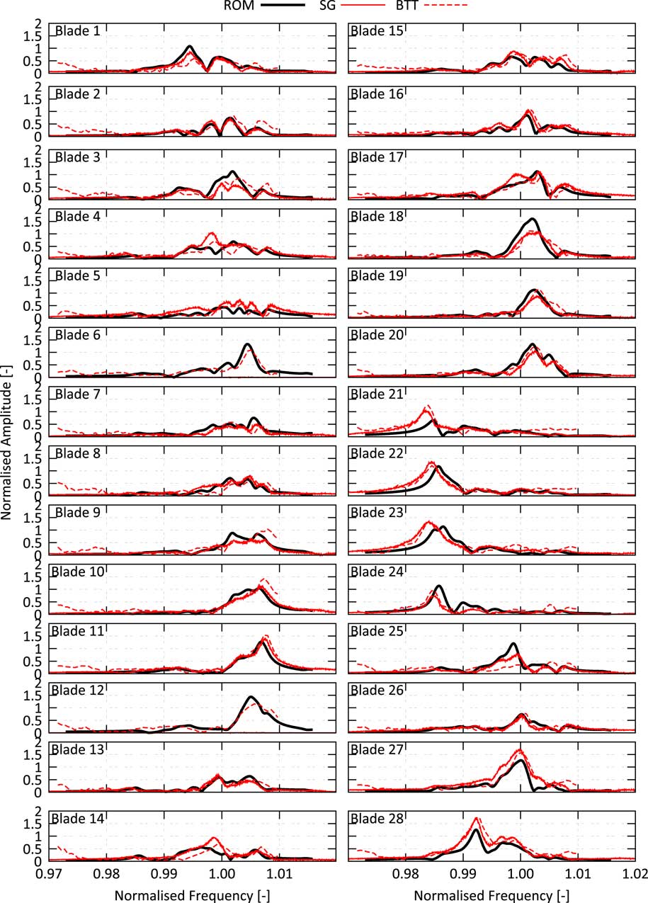
The good overall agreement is also observed for predicted and measured FRFs, see Fig. 20. The amplitude and damping level, the frequencies of the maximum vibration response and also cancellations in between the resonances are very well predicted. Remaining discrepancies on some of the blades might be due to slight differences in the operating conditions (e.g. working line or speed), the idealised geometry (e.g. simplified penny gaps, the usage of ideal CAD geometry for all vanes and blades and the omitted influence of the instrumentation like kielheads, pressure taps or SGs), the simple Spalart–Allmaras turbulence model (especially for the separated flow at resonance condition 1), and finally possible small deviations of the actual mistuning distribution from the measured one. Considering all these uncertainties, the prediction is in very good agreement with the measurement, and it can be concluded that both rig test and prediction provided proof of the presence of TSM excitation and its remarkable effect on the forced response.

Figure 20 Comparison of measured and predicted frequency response functions for the resonance condition 1 (80% VSV schedule).
3.0 CONCLUSIONS
The aim of this study was to contribute to a better understanding of TSM excitation and its effect on the mistuned forced response. In order to cover this demand, the theoretical explanation, the physics involved in the generation of TSM as well as the effect of the upgraded right-hand side on the forced response have been reviewed. This mostly theoretical review has been supported with unsteady simulations of a quasi 2D section of a multistage engine to visualise the abstract formulation. This study revealed that though TSMs are also present in single stage engines, it needs a multistage engine for the generated TSM to lead to blade individual forces on the affected rotor. This blade individual force leads to harmonic components with wave numbers being multiples of the rotor blade difference to appear in the amplitude vs blade pattern. The blade individual amplification of its vibration level is also present for the tuned rotor. Due to the structural coupling of the blades, the effect of blade individual force may not necessarily lead to a significant amplification of the forced response level. The amplification of the vibration level is also a function of the damping ratio and frequency spread of the excited system modes.
The second part of this study shifted the focus on the forced response of the Rotor 2 blisk in an 4.5-stage research compressor. The idea was to study the mechanical resonance of mode 11 with EO36 in two different flow conditions in order to separate the influence of the TSMs from the impact of mistuning. This has been accomplished by the application of two different VSV schedules. The structural behaviour is simulated by an SNM representation of the mode family 11 which has been validated at rest by means of comparing predicted and measured mistuned mode shape envelopes( Reference Beirow, Kühhorn, Figaschewsky, Hönisch, Giersch and Schrape 12 ). This ROM considers mistuning, gyroscopic loads as well as aerodynamic damping and is derived from an FE sector model taking into account the impact of the assembled drum on the structural dynamics. Unsteady CFD simulations of the full circumference of the front block of the compressor (Strut, IGV, R1, S1, R2, S2, R3, S3) have been used to calculate the aerodynamic force for the two different VSV schedules. These simulations indicate a remarkable increase in the strength of the TSMs when shifting from the VSV80 to the VSV90 case.
At the same time, the aerodynamic damping does not change significantly (+25%) i.e. a traditional forced response analysis with only the single dominant TWM included in the right-hand side indicated almost no change of the amplitude vs blade pattern normalised by the mean value. Contrarily, the rig test revealed a remarkable change of the pattern. The shape of the observed change in the patterns features a dominant wave number equal to the difference of the number of blades of R1 and R2 and agrees well with the theoretical predictions. By applying the calculated TSMs to the aeromechanical model, a very similar effect on the forced response has been predicted. Also, the measured and predicted FRFs are in very good agreement. Hence, the investigation provides proof of the presence of TSMs in multistage engines as well as its influence on the forced response. Furthermore, it has been shown that the effect can be adequately predicted by suitable aeromechanical models. Both results are assumed to advance the state of the art in forced response analyses.
ACKNOWLEDGEMENTS
The investigations contribute to the research project AeRoBlisk (FKZ: 20T0901C) which is funded by the German Federal Ministry of Economics and Technology. The authors gratefully acknowledge Rolls-Royce Deutschland Ltd & Co KG and the German Aerospace Center (DLR) for granting permission for its publication, their support and for providing the rig test measurement data.