1. Introduction
Autonomous unmanned aerial vehicles (UAVs) have attracted much attention from industries and defence over the past several decades. With advances in low-cost inertial sensor technology and the global navigation satellite system (GNSS), the navigation solution (position, velocity, attitude and time) can be accurately estimated by integrating the information. This data fusion approach has enabled higher-level autonomy, such as intelligent path planning and decision making (Parkinson, Reference Parkinson1997; Kim et al., Reference Kim, Sukkarieh and Wishart2003; Skulstad et al., Reference Skulstad, Syversen, Merz, Sokolova, Fossen and Johansen2015).
One of the key challenges in achieving reliable navigation solutions has been in handling signal interference, both intentional (such as jamming or spoofing) or unintentional (multipath or blockage), which can degrade satellite-based aiding of the low-cost inertial system. This interference problem has been addressed at various levels, such as the low-level design of a signal tracking loop to the high-level fusion of redundant information. Recently, simultaneous localisation and mapping (SLAM) has drawn much attention as an alternative aid to inertial systems. For example, Kim and Sukkarieh (Reference Kim and Sukkarieh2003, Reference Kim and Sukkarieh2007) demonstrated the integration of an inertial measurement unit (IMU) and an inertial navigation system (INS) as core odometry together with visual perception sensor on a UAV platform. Nützi et al. (Reference Nützi, Weiss, Scaramuzza and Siegwart2011) integrated monocular vision and an inertial sensor on a drone platform addressing the monocular scale ambiguity problem. Li and Mourikis (Reference Li and Mourikis2013) showed visual–inertial odometry and SLAM by utilising a sliding-window-based bundle adjustment optimisation on a six-degrees-of-freedom vehicle. Sjanic et al. (Reference Sjanic, Skoglund and Gustafsson2017) applied the expectation-maximisation technique for visual–inertial navigation of fixed-wing flight data. Recently, Vidal et al. (Reference Vidal, Rebecq, Horstschaefer and Scaramuzza2018) demonstrated a high-speed drone by combining an event camera and inertial observations.
Although the above-mentioned approaches have been quite promising, achieving reliable and efficient SLAM solutions on high-speed UAV platforms has had limited success, which is largely due to the low-quality inertial odometry and the high computational complexity inherent to SLAM. In particular, the flight dataset we consider in this work has very sparse landmark observations (typically fewer than three landmarks per camera frame). Thus aiding the inertial navigation solution using sparse visual observations under a reduced number of satellite vehicles becomes highly challenging.
To address this problem, we propose a novel all-source navigation filter, termed compressed pseudo-SLAM (CP-SLAM), which can seamlessly integrate all available observations in a computationally efficient way. The closest work to ours is Williams and Crump (Reference Williams and Crump2012), which demonstrated the all-source navigation strategy on a UAV platform by fusing GNSS, IMU and camera information within the SLAM framework. However, the SLAM architecture relies on a standard extended Kalman filter (EKF), which has a high computational complexity of $\mathcal {O}(N^{2})$ , with $N$
 being the total number of registered landmarks. In our approach, a local map is dynamically defined around the vehicle, and only the local landmarks within the region are actively updated within the filter. The global landmarks are only updated at a much lower rate by compressing the local-to-global correlation information. Owing to this compressed filtering approach, the complexity reduces to $\mathcal {O}(L^{2})$
 , with $L$
 being the number of local landmarks, which is much smaller than the total number $N$
 . This work extends the previous work by Kim et al. (Reference Kim, Cheng, Guivant and Nieto2017), which was a simulation-based study. The contributions of this work are twofold:
• Demonstration of the CP-SLAM for a high-speed, fixed-wing UAV dataset.
• Evaluation of the CP-SLAM performance with a reduced number of satellites and sparse visual observations.
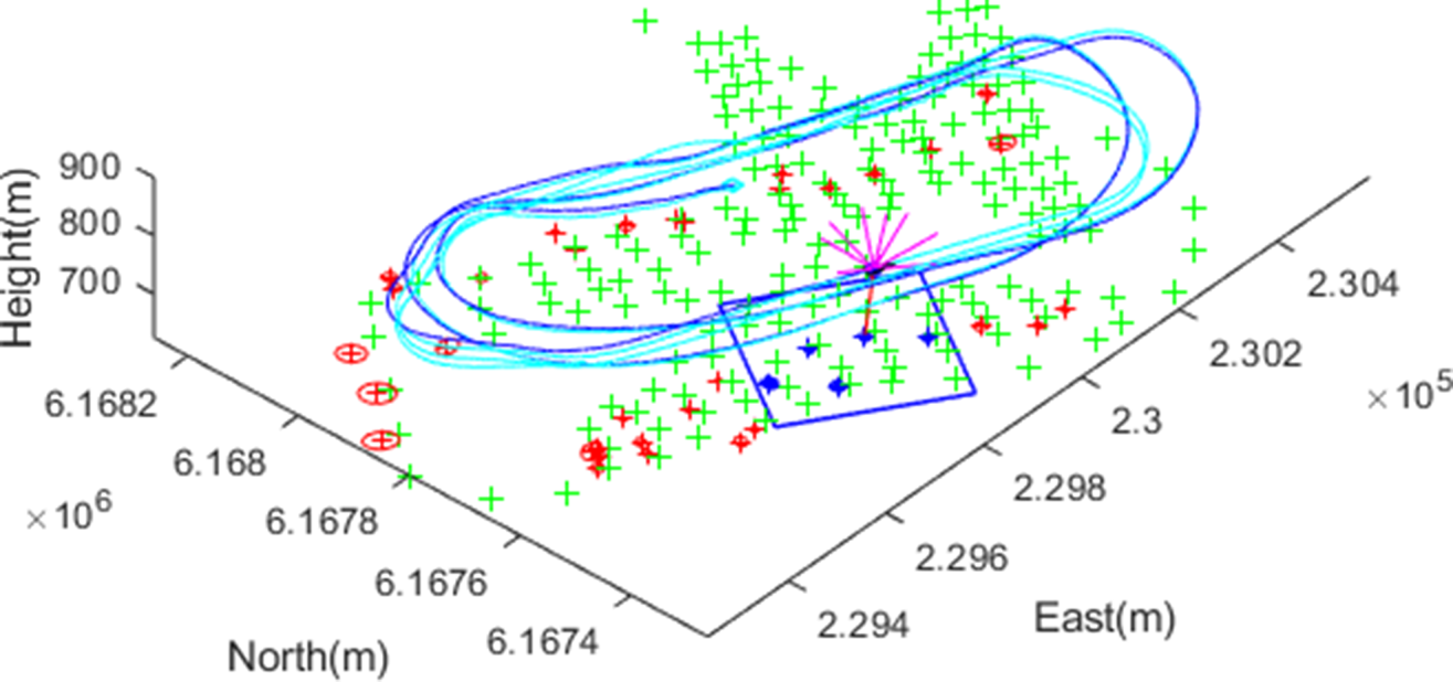
Figure 1 illustrates a snapshot (a movie clip is availableFootnote 1 ) of the CP-SLAM operation, showing GNSS pseudorange measurements from satellite vehicles (SVs) shown as magenta-coloured lines pointing upwards from the vehicle, and a visual landmark observation as a red-coloured line pointing downwards from the vehicle, along a racehorse trajectory. Onboard navigation solutions recorded from a loosely-coupled Global Positioning System (GPS)/INS system are also shown in cyan, together with the surveyed landmark positions (‘$+$ ’ marks in green). The key features in this work are: (1) the seamless aiding of inertial navigation from the pseudorange/pseudorange rates and the visual observations in a unified framework, and (2) the computationally-efficient compressed filtering, partitioning the map into local (the blue box on the plot) and global (red points) ones. Thanks to the compressed approach, the global map is updated much less frequently whenever the local map is redefined, providing the computational benefits compared to the full-rate global update. To the best of our knowledge, this is the first UAV flight result integrating the pseudoranges and visual observations in a compressed filtering framework.

Figure 1. A snapshot of the compressed pseudo-SLAM (CP-SLAM) for fixed-wing UAV navigation. The line-of-sight vectors to nine satellite vehicles are shown as lines pointing upwards (in magenta) from the vehicle, and one visual feature observation is shown downwards (in red). The blue box shows an adaptive local map boundary, including active landmarks with uncertainty ellipses (in blue), while the red ellipses are for the global (inactive) landmark states. As the ground truth, surveyed landmark locations are shown as green ‘$+$ ’ marks, as well as the onboard GPS/INS solution in cyan colour
The remainder of the paper is outlined as follows. Section 2 provides the system models for the nonlinear state transition and observation used in this work, and Section 3 details the compressed pseudo-SLAM with a compressed update of the local and global map. Experimental results are provided in Section 4, analysing the filter performance and the computational complexity. Section 5 will conclude with future directions.
2. System models
A continuous-time stochastic dynamic system with a nonlinear transition model $\mathbf {f}(\cdot )$ and an observation model $\mathbf {h}(\cdot )$
 can be written as


where $\mathbf {x}(t)$ and $\mathbf {u}(t)$
 are the state and control input vectors at time $t$
 , respectively, with $\mathbf {w}(t)$
 being the process noise with a noise strength matrix $\mathbf {Q}$
 , and $\mathbf {z}(t)$
 is the observation vector with $\mathbf {v}(t)$
 being the observation noise with a strength matrix of $\mathbf {R}$
 .
.
In the inertial-based SLAM, the state vector consists of a vehicle state that represents the kinematics of the inertial navigation, inertial sensor errors and map landmark states. In this work, a $17$ -state model is designed to estimate the vehicle position and attitude (six), velocity and sensor biases (nine) and receiver clock states (two), as well as the variable-size map states. The control input is the IMU measurements and drives the inertial kinematic equations. Thus the state vector $\mathbf {x}=(\mathbf {x}_v^\textrm {T}, \mathbf {m}^\textrm {T})^\textrm {T}$
 becomesFootnote 2


where
• vehicle position in the navigation frameFootnote 3 $\mathbf {p}^{n} = ( x, y, z )$
 ,
,• vehicle velocity $\mathbf {v}^{n} = ( v_x, v_y, v_z )$
,• vehicle attitude (Euler angles in roll, pitch and yaw) $\boldsymbol {\psi }^{n} = ( \phi , \theta , \psi )$
,• accelerometer bias in the body frameFootnote 4 $\mathbf {b}^{b}_a =( b_{ax}, b_{ay}, b_{az} )$
,• gyroscope bias $\mathbf {b}^{b}_g = ( b_{gx}, b_{gy}, b_{gz})$
,• receiver clock bias ${ct}_{b}$
, with $c$ being the speed of light,• receiver clock drift ${ct}_{d}$
,• map position $\mathbf {m}^{n}_i = (m_{ix}, m_{iy}, m_{iz})$
,• accelerometer measurement $\mathbf {f}^{b} = (f_x, f_y, f_z)$
and• gyroscope measurement $\boldsymbol {\omega }^{b} = (\omega _x, \omega _y, \omega _z )$
.


2.1 Dynamic model
The system dynamic model consists of the kinematic equations of the inertial navigation driven by the IMU measurements, which are the specific force (or the sum of dynamic acceleration of the vehicle and gravity) and angular rate. The IMU bias errors are modelled as a random walk process, while the map states are modelled as a random constant due to their stationary nature, yielding


where
• $\boldsymbol {\omega }^{n}_{ie}$
is the Earth's rotation rate in the navigation frame,• $\mathbf {g}^{n}(\mathbf {{p}}^{n})$
is the gravitational acceleration,• $\mathbf {w}_a$
, $\mathbf {w}_g$ and ${w}_d$ are noise processes for accelerometers, gyroscopes and receiver clock drift, respectively, and• $\mathbf {C}_{b}^{n}$
and $\mathbf {E}_{b}^{n}$ are the direction cosine matrix transforming a vector in the body frame to that in the navigation frame, and the matrix transforming a body rate to an Euler angle rate, respectively,
\begin{align*} \mathbf{C}_{b}^{n}& =\left[ \begin{array}{ccc} c_\theta c_\psi & -c_\phi s_\psi + s_\phi s_\theta c_\psi & s_\phi s_\psi + c_\phi s_\theta c_\psi \\ c_\theta s_\psi & c_\phi c_\psi + s_\phi s_\theta s_\psi & -s_\phi c_\psi + c_\phi s_\theta s_\psi \\ -s_\theta & s_\phi c_\theta & c_\phi c_\theta \end{array}\right],\\ \mathbf{E}_{b}^{n} &=\left[ \begin{array}{ccc} 1 & s_\phi t_\theta & c_\phi t_\theta \\ 0 & c_\phi & -s_\phi \\ 0 & s_\phi/c_\theta & c_\phi/c_\theta \end{array}\right], \end{align*}where $s_{(\cdot )}$
, $c_{(\cdot )}$ and $t_{(\cdot )}$ are shorthand notation for $\sin (\cdot )$, $\cos (\cdot )$ and $\tan (\cdot )$, respectively.


Please note that this utilises a simplified version of the strap-down inertial navigation equations, aiming for low-cost inertial system applications. The effects of the Earth's curvature on the attitude calculation are not included, although it will be straightforward to add the curvature terms in the model.
2.2 Observation model
In the all-source aiding strategy, the observations consist of all available aiding information, which, in this work, is a set of pseudoranges ($\rho$ ) and pseudorange rates ($\dot {\rho }$
 ) measured from a GNSS receiver, and/or a set of range $r$
 , bearing $\phi$
 and elevation $\theta$
 observations from a camera sensor:


Here $(X_i, Y_i, Z_i)$ denotes the $i$
 th SV's position computed from the ephemeris data, which is converted from the ECEF (Earth-Centred, Earth-Fixed) frame to the navigation frame, with $v_\rho$
 being the noise process, and $(l_{xi}, l_{yi}, l_{zi})$
 is the line-of-sight vector of the $i$
 th SV seen from the vehicle, which projects the relative velocity along the line-of-sight direction. For the range, bearing and elevation measurement, we first compute the relative position vector $((m_{jx}-x), (m_{jy}-y), (m_{jz}-z) )$
 of the $j$
 th landmark seen from the vehicle, and then transform it to polar coordinate quantities. Finally, $(v_\rho , v_{\dot \rho }, v_r, v_\phi , v_\theta )$
 represent the observation noise processes. A new landmark position is initialised by utilising the inverse function of Equations (14) to (16) with the estimated vehicle state and observation information.
3. Compressed pseudo-SLAM
Using the state and observation models described in the previous section, and their corresponding linearised state and observation models ($\mathbf {F}, \mathbf {H}$ ), a standard EKF can predict and update the state and covariance matrix ($\mathbf {P}$
 ) as detailed in Kim and Sukkarieh (Reference Kim and Sukkarieh2007). In a compressed filtering framework, the state vector is further partitioned into (1) a local map state including the vehicle state and local map, and (2) a global map for the remaining landmarks (Guivant, Reference Guivant2017; Kim et al., Reference Kim, Cheng, Guivant and Nieto2017). The underlying key assumption is that the cross-correlation information is only dependent on the local states, thus enabling accumulation (thus compression) during the local filtering cycles. Consequently, the compressed cross-correlation can be used to update the global state at a much lower rate. This assumption is quite valid for the downward-looking camera configuration, as in this work, where the camera field of view naturally defines the minimum boundary of the local map. The partitioned state estimates and covariance matrix become


where the local estimate $\hat {\mathbf {x}}_L$ includes the vehicle $\hat {\mathbf {x}}_v$
 and local landmarks $\hat {\mathbf {m}}_{L}$
 , while the remaining landmarks are stacked as $\hat {\mathbf {m}}_G$
 .
.
In the compressed prediction step, the vehicle-to-map correlation is compressed as

where $\boldsymbol {F}(s)$ is the Jacobian matrix at a discrete step $s$
 with a step time $\Delta T$
 . In this work, the prediction rate is $400$
 Hz driven by the IMU data, and the correlation information is accumulated until a local-to-global update event occurs, which is at much lower rate of around $0{\cdot }5$
 Hz in this work. This is a significant computational gain in the SLAM prediction, as only the $17\times 17$
 vehicle-dependent Jacobian matrix needs to be compounded at a full rate, compared to the full correlation update of $17 \times N$
 or full covariance of $N \times N$
 .
.
When observations are available (either pseudoranges/rates at $1$ Hz or visual landmarks at $25$
 Hz), the local filter states are first updated, then the cross-correlation term $\mathbf {P}_{LG}$
 and finally the full global states. In compressed filtering, the accumulated cross-correlation at discrete time $k$
 has a closed-form expression given the initial correlation $\mathbf {P}_{LG}(0)$
 as
as

where the terms inside the product are all available from the local filter update – the observation Jacobian $\mathbf {H}(s)$ , the innovation covariance $\boldsymbol {S}(s)$
 and the local covariance $\boldsymbol {P}_{LL}(s)$
 .
.
By using this compressed correlation $\mathbf {P}_{LG}(k)$ , the global map and covariance matrix can be recovered as


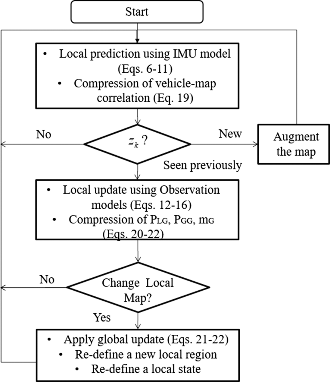
where $\boldsymbol {\nu }(s)$ represents the local innovation during the local update. Figure 2 summarises the algorithmic flow diagram with the key relevant equations discussed in this section. More discussions are provided in the following results section, such as the data association and local region selection methods.

Figure 2. The flow diagram of the CP-SLAM algorithm
4. Experimental results
4.1 Environment and sensors
A flight dataset recorded from a fixed-wing UAV platform (Kim and Sukkarieh, Reference Kim and Sukkarieh2007) is used to verify the method. An IMU sensor is a low-grade sensor with a gyroscope bias stability of $10^{\circ }/\textrm {h}$ , delivering outputs at $400$
 Hz. A GPS receiver from Canadian Marconi Communication (now NovAtel) was used to record the pseudorange and pseudorange rate measurements at $1$
 Hz and the satellite ephemeris data. The receiver provides integrated-carrier-phase (ICP) measurements, which are used to compute the pseudorange rates. Differential GPS (DGPS) correction messages (Radio Technical Commission for Maritime Services; RTCM) were broadcast from the ground station at the time of the experiment. A Sony monochrome camera (with a frame rate of $25$
 Hz) was installed in a down-looking configuration. Please refer to Kim and Sukkarieh (Reference Kim and Sukkarieh2007) for more details of the onboard sensor configurations together with a flight control computer that recorded the data.
Figures 3(a) and 3(b) show sample aerial images collected from the camera, showing a white landmark laid on the ground at the bottom right corner of Figure 3(b). These artificial visual landmarks are made of white plastic sheets ($1\ \textrm {m} \times 1\ \textrm {m}$ ). They are installed on the ground, whose positions are pre-surveyed using a pair of real-time-kinematic GPS receivers. An intensity-based blob-detection algorithm is used, followed by template matching to detect square-shaped landmarks. Once detected, the known size of white pixels is used to compute the distance (range) to the landmark. The resulting (range, bearing, elevation) with uncertainty are reported/recorded in the camera coordinate system as shown in Figures 3(c) and 3(d). It can be observed that landmarks are first detected from the top of the camera image (or with the minimum elevation angle in the camera coordinates), tracked and disappeared at the bottom of the image (or with the maximum elevation angle). This can be seen in the increasing elevation angles in Figure 3(d). The range also shows a ‘V’-like pattern, which stems from the fact that the distance to a landmark becomes minimum when the landmark lies directly under the vehicle. The detected landmarks are associated with the SLAM map using the joint-compatibility branch and bound (JCBB) algorithm, which can effectively match a set of landmarks with the map. In this work, however, the number of landmarks detected in each image frame is quite low (one or two), and thus the association performance is close to the nearest-neighbour (NN) method.
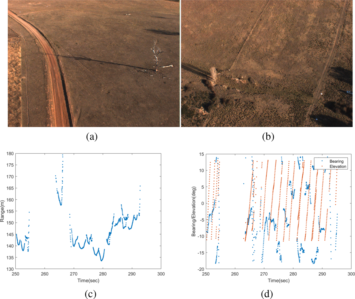
Figure 3. (a,b) Two aerial images seen from the UAV. In (b) an artificial/white visual landmark is seen in the bottom right corner of the image, which is a white plastic sheet of $1\ \textrm {m} \times 1\ \textrm {m}$ from which the range was estimated. (c) Extracted range and (d) bearing/elevation measurements from the detected visual landmarks. It can be observed that landmarks are detected from the top of the camera image (with a minimum elevation angle) and exit the view at the bottom of the image (with a maximum elevation angle). This also manifests in the range showing ‘V’-like patterns, which stems from the fact that the range becomes maximum when a landmark is first or last detected, while it is a minimum when it is directly under the vehicle
4.2 Flight trajectory and vertical stabilisation
The flight segment has around $6$ min of duration from taking off, along the multiple racehorse trajectories (each track is about $5$
 km long). The average flight speed is around $120$
 km/h, and the average altitude is $150$
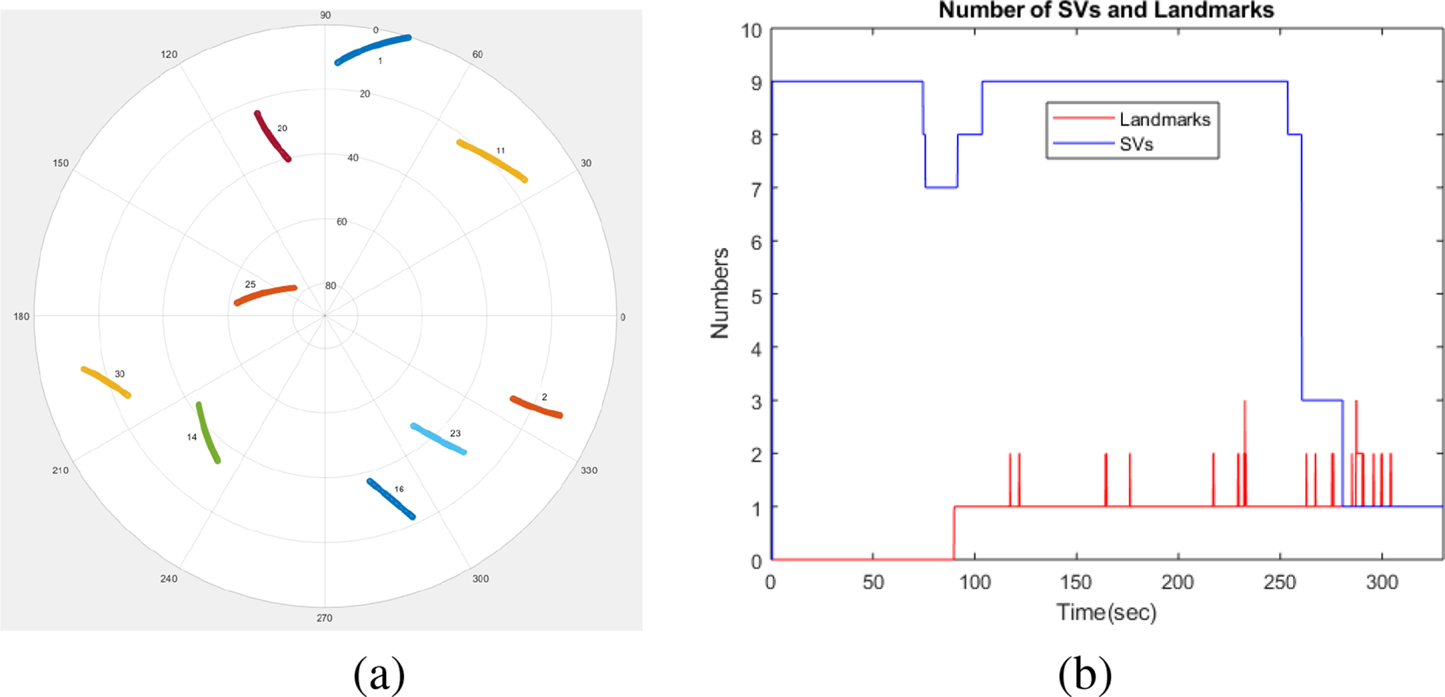
 m above the ground. Figure 4(a) shows the sky plot of the visible SVs in an azimuth–elevation form showing nine visible SVs. Figure 4(b) shows the change of the number of SVs during the flight, with a simulated drop to three from $250$
 s and then one from $280$
 s to test the performance of the system. The number of visual landmarks (in red) is also shown, which changes from zero to three during the flight. These sparse visual observations make the height aiding of the inertial navigation system particularly challenging due to the large range errors inherent to the visual sensing. In this work, we stabilise the vertical height using the additional barometric-altitude information. The absolute and relative pressure measurements from the air data system are converted to barometric height and climb rate and then used to aid the vertical inertial outputs using a simple $\alpha$
 –$\beta$
 filter. Although this is a suboptimal approach, it simplifies the SLAM filter tuning process with reliable performance and is thus adopted in this work.

Figure 4. (a) The sky view plot of the satellite vehicle during the flight experiment. (b) A dropout of the satellites from $250$ s was simulated. The number of visual landmarks is also shown. It can be observed that the number of visual landmarks is quite low, changing from zero to three, and thus requires additional pseudorange information to calibrate the low-cost IMU
4.3 CP-SLAM performance
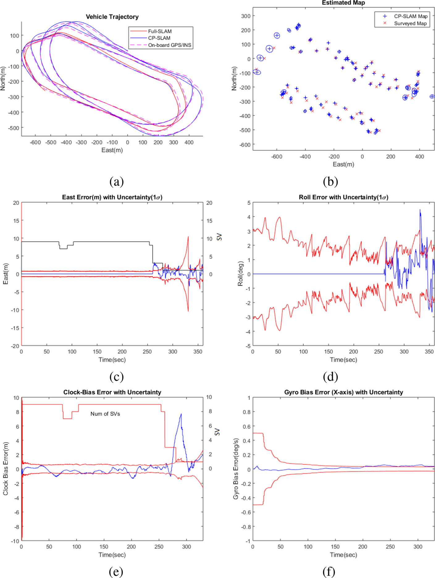
Figures 1 and 5 illustrate the operation of the CP-SLAM system and the estimation results, respectively. Figure 5(a) compares the estimated vehicle positions from CP-SLAM (in solid blue), non-compressed Full-SLAM (in solid red) and on-board GPS/INS solution (in dashed red). It can be seen that the CP-SLAM and Full-SLAM show almost identical accuracy. Figure 5(b) also compares the estimated map from the CP-SLAM and the ground truth (surveyed map) with a total of $85$ landmarks and uncertainty, showing consistent mapping performance.

Figure 5. The estimation results from the compressed pseudo-SLAM (CP-SLAM): (a) the vehicle trajectory compared with Full-SLAM and on-board GPS/INS solution; (b) the map with uncertainty ($10\sigma$ for visual clarity); (c) the East positional error (m) with uncertainty ($1\sigma$
 ); (d) the roll angular error (deg) with uncertainty ($1\sigma$
 ); (e) the receiver clock-bias error (m) with uncertainty ($1\sigma$
 ); and (f) the $x$
 -gyro bias error with uncertainty ($1\sigma$
 ). The CP-SLAM trajectory shows a consistent result compared to Full-SLAM. The navigational errors and corresponding uncertainties show larger errors when the number of SVs drops to three and one. However, thanks to the continuous SLAM aiding, the navigational/clock/sensor errors are all constrained adequately
Figure 5(c) presents the navigational errors (East position error and roll angle error) with $1\sigma$ uncertainties, and Figure 5(f) shows the receiver clock bias error and the IMU gyroscope bias error ($x$
 -axis) with uncertainties. It can be observed that, when the number of SVs is sufficiently large (more than four), the pseudorange measurements dominate the estimation performance. In contrast, when the number of SVs drops to three and one, the errors increase, but the errors are adequately constrained within the uncertainty bound thanks to the continuous visual aiding.
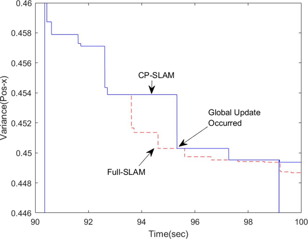
Figure 6 compares the evolution of the map covariance from CP-SLAM (in solid blue) and Full-SLAM (in dashed red). For the clarity of the plot, only the result of landmark 1 is shown for the first $10$ s from the initial registration. It can be seen that, during $90{\cdot }5$
 –93 s, the landmark is within the local map, thus actively updated in both CP-SLAM and Full-SLAM. However, from $93$
 s onwards, the landmark becomes inactive, as it is out of the local map, making CP-SLAM's covariance unchanged. In contrast, the Full-SLAM continuously reduces the covariance. Owing to the global updates at around $95$
 s and $99$
 s, the whole map is corrected, making the CP-SLAM results back to optimal, thanks to the compressed fusion method. This clearly demonstrates CP-SLAM's benefits, which can run the global update less frequently without sacrificing performance. This result is consistent with the results of Guivant (Reference Guivant2017, see Figure 3 on page 13), which utilised simulated multiple mobile robots showing that the CP-SLAM methods can be generalisable to various robot navigation problems.

Figure 6. Comparison of the evolutions of covariance of CP-SLAM (in solid blue) and Full-SLAM (in dashed red), for landmark 1. Landmark 1 is first registered at around $90{\cdot }5$ s, and the covariance of CP-SLAM and Full-SLAM change in the same way as the landmark is within the active map. From $93$
 s, however, the landmark becomes inactive, as it is out of the local map, making the covariance of CP-SLAM unchanged. In contrast, the Full-SLAM continuously reduces the covariance. Owing to the global updates at around $95$
 s and $99$
 s, the whole map is corrected, making the CP-SLAM results back to optimal, thanks to the compressed fusion method
4.4 Computational complexity
Figure 7(a) presents the change of the total number of landmarks (in blue) and the number of local landmarks (in red) registered in the CP-SLAM filter. The final state vector dimension is $272$ , consisting of the vehicle states ($17$
 ) and the landmark maps ($255$
 ), which corresponds to $85$
 landmarks with three-dimensional position for each landmark. The number of local landmarks is maintained within $20$
 throughout the flight, although it increases towards the end of the flight. This increase was due to the higher altitude of the vehicle resulting in a bigger local map and thus more local landmarks.
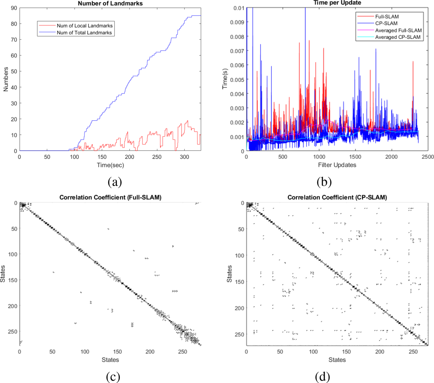
Figure 7. (a) Comparison of the total number of landmarks registered (in blue) and the number of local landmarks in CP-SLAM (in red), and (b) comparison of the update time of the Full-SLAM (in red) and CP-SLAM (in blue). The smoothed average values of the update times clearly show the benefits of the CP-SLAM. (c) Full-SLAM's correlation coefficient matrices and (d) CP-SLAM (the vehicle states correspond to the top-left elements in the matrix). Both matrices show strong diagonal correlation patterns but with sparse off-diagonal structures due to the loop closures. CP-SLAM shows more off-diagonal elements, which are due to the frequent reshuffling of the landmarks into the local and global ones, but has a smaller band-diagonal pattern due to the lower number of local landmarks
Figure 7(b) compares the computational times of the filter update from CP-SLAM (in blue) and Full-SLAM (in red), showing the improved computational performance of CP-SLAM. The Full-SLAM update's computational complexity is $\mathcal {O}(N^{2})$ , with $N$
 being the total number of landmarks. At the same time, the CP-SLAM has the complexity of $\mathcal {O}(L^{2}),\ L\ll N$
 , with $L$
 being the local map size, which is less than the total map size. We can see that the pseudorange update times are nearly constant with $1$
 ms on average, while the local landmark update times increase towards $1{\cdot }5$
 ms. However, the local-to-global updates sometimes show peaks during the map transitions, which was affected by the additional data association and sorting process. During the last $60$
 s of the GNSS dropout period, the update time is dominated by the visual updates. This result confirms that the compressed filtering approach is suitable for the real-time processing showing on average $1{\cdot }5$
 ms processing time (using MATLAB on an Intel i5-core CPU with $1{\cdot }7$
 GHz).
GHz).
Figures 7(c) and 7(d) further compare the correlation structures of the Full-SLAM and CP-SLAM. Owing to the sparse visual observations and landmarks, the correlation coefficient matrices become sparse (the top left corner blocks are for the vehicle states). The Full-SLAM contains a much wider band-matrix structure than the CP-SLAM, particularly towards the bottom right blocks, as expected. The CP-SLAM shows more off-diagonal elements, which are due to the frequent reshuffling of the landmarks into the local and global ones, but has a smaller band-diagonal pattern due to the lower number of local landmarks. It can be noted that Full-SLAM registers the landmarks in temporal order, while CP-SLAM reorders the map based on spatial closeness. Depending on the application, we can apply a more optimal strategy to define the local map. For example, this work utilises a moving local region along with the vehicle, while Guivant (Reference Guivant2017) used a grid-based and fixed local region resulting in more block-diagonal structures. A further investigation might lead to a more sparse structure and thus a more efficient filtering algorithm.
5. Conclusions
This paper presented a novel compressed pseudo-SLAM algorithm that seamlessly integrates pseudorange/pseudorange rates and inertial–visual SLAM to achieve continuous and reliable UAV navigation in a partially GNSS-denied environment. A flight dataset recorded from a high-speed, fixed-wing UAV platform was used to demonstrate the method. The offline processed results using MATLAB showed sustained and reliable navigation solutions even under a single SV and sparse landmark observations while calibrating the IMU and the receiver clock errors. The compressed implementation improved the computational complexity, achieving a filter update time of less than $1{\cdot }5$ ms on average for the state dimension of $272$
 , consisting of $17$
 for the vehicle states and $255$
 for the map (or $85$
 landmarks). This result confirms the feasibility of the method for real-time implementation, which is a future work using a drone platform. The performance can be further improved by investigating the satellites’ and landmarks’ optimal sensing geometry and designing an efficient local map strategy. Future work is to address how to optimally select the ground landmarks given a set of satellites in a cluttered environment to complement the low GNSS accuracy, for example, height.
Acknowledgments
The authors thank the Australian Centre for Field Robotics (ACFR) for the use of the flight dataset in this paper.
Funding statement
This research was supported by ARC Discovery Project grant (DP200101640) and Research Council of Norway grant numbers (223254 and 250725).