


1 Introduction
Transition to turbulence of the boundary layers on a hypersonic vehicle can greatly enhance surface heating rates and increase frictional drag; understanding and prediction of boundary-layer transition is thus a critical problem in hypersonic flight. It is now well established that, because of variations in the free stream disturbance levels between conventional ground-test facilities and flight, simple correlations of transition locations from experiments are inadequate for extrapolation to flight (Reshotko Reference Reshotko1976; Schneider Reference Schneider2001) and that measurements of the boundary-layer instabilities leading to transition are required to make meaningful progress. In order to reproduce true hypervelocity conditions and the accompanying high-temperature effects in ground-based testing, the use of impulse facilities such as reflected-shock wind tunnels and expansion tubes is necessary. Because of the short test times and harsh flow environments intrinsic to these facilities, however, the difficulty in making instability measurements is greatly increased compared to cold hypersonic tunnels, i.e. facilities that simulate flight Mach numbers but not velocities.
For hypersonic flows over slender two-dimensional or axisymmetric geometries at zero or small angles of incidence, the dominant instability is typically what is referred to as the inviscid second or Mack mode (Mack Reference Mack1975), though Fedorov & Tumin (Reference Fedorov and Tumin2011) point out that it is not a true mode in the mathematical sense of the word. Physically, second-mode disturbances can be thought of as trapped acoustic waves inside the boundary layer. They propagate downstream with a phase speed close to the boundary-layer edge velocity and have a wavelength two to three times the boundary-layer thickness, resulting in dominant frequencies ranging from approximately 100 kHz to over 1 MHz, the latter for hypervelocity, high Reynolds number boundary layers. The accurate measurement of instability wave properties at this upper frequency limit presents a significant challenge; for this reason, early experimental investigations of hypervelocity boundary-layer transition focused primarily on measurements of transition location and correlating this with the flow enthalpy.
He & Morgan (Reference He and Morgan1994) performed measurements on a flat plate in the T4 shock tunnel at the University of Queensland and found the transition Reynolds number to decrease with increasing enthalpy. Adam & Hornung (Reference Adam and Hornung1997) and Germain & Hornung (Reference Germain and Hornung1997) determined approximate laminar–turbulent transition locations on a sharp 5°-half-angle cone using various test gases in the GALCIT T5 shock tunnel. These latter authors found little evidence of a trend when the transition Reynolds number based on boundary-layer edge conditions was plotted against the enthalpy. When the Eckert reference temperature was used to calculate the transition Reynolds number,
 $Re_{tr}^{\ast }$
, however, two notable trends emerged. First, regardless of the test gas,
$Re_{tr}^{\ast }$
, however, two notable trends emerged. First, regardless of the test gas,
 $Re_{tr}^{\ast }$
increased with increasing enthalpy (over a certain, gas-specific range of enthalpy). Second, the rate of increase in
$Re_{tr}^{\ast }$
increased with increasing enthalpy (over a certain, gas-specific range of enthalpy). Second, the rate of increase in
 $Re_{tr}^{\ast }$
was strongly dependent on the test gas over the range of tested conditions: for nitrogen, only a weak increase was observed, but this became somewhat stronger for air and even more so for carbon dioxide. These differences were suggested to arise from the varying temperatures at which non-equilibrium effects (vibrational and/or dissociational) became important in these three gases. Furthermore, it was hypothesized that the increasing
$Re_{tr}^{\ast }$
was strongly dependent on the test gas over the range of tested conditions: for nitrogen, only a weak increase was observed, but this became somewhat stronger for air and even more so for carbon dioxide. These differences were suggested to arise from the varying temperatures at which non-equilibrium effects (vibrational and/or dissociational) became important in these three gases. Furthermore, it was hypothesized that the increasing
 $Re_{tr}^{\ast }$
trend was caused by damping of the second-mode waves thought to be responsible for transition, since the second mode is acoustic in nature and acoustic waves can be attenuated by non-equilibrium processes (Clarke & McChesney Reference Clarke and Mcchesney1964). This interpretation was given further support by the linear stability analysis of Johnson, Seipp & Candler (Reference Johnson, Seipp and Candler1998), who showed reacting disturbances generally to have lower amplification rates than non-reacting disturbances at the conditions employed in the T5 experiments. This was a significant finding as earlier computational work by Malik & Anderson (Reference Malik and Anderson1991), concentrating on the stability of the mean flow, had indicated that real gas effects tended to destabilize the second mode at similar conditions. An investigation of the effects of rotational non-equilibrium by Bertolotti (Reference Bertolotti1998) showed this also to lead to damping of second-mode disturbances.
$Re_{tr}^{\ast }$
trend was caused by damping of the second-mode waves thought to be responsible for transition, since the second mode is acoustic in nature and acoustic waves can be attenuated by non-equilibrium processes (Clarke & McChesney Reference Clarke and Mcchesney1964). This interpretation was given further support by the linear stability analysis of Johnson, Seipp & Candler (Reference Johnson, Seipp and Candler1998), who showed reacting disturbances generally to have lower amplification rates than non-reacting disturbances at the conditions employed in the T5 experiments. This was a significant finding as earlier computational work by Malik & Anderson (Reference Malik and Anderson1991), concentrating on the stability of the mean flow, had indicated that real gas effects tended to destabilize the second mode at similar conditions. An investigation of the effects of rotational non-equilibrium by Bertolotti (Reference Bertolotti1998) showed this also to lead to damping of second-mode disturbances.
While the experimental studies just described gave valuable qualitative information regarding hypervelocity boundary-layer transition, more recently it has been recognized that to provide experimental confirmation of these computational predictions, measurements of the instabilities themselves rather than simple transition locations are required (in line with the point made in the first paragraph). This has led to efforts by groups at several shock tunnels worldwide - notably, T5 at the California Institute of Technology, the CUBRC facilities at Buffalo, HIEST at JAXA and HEG at the German Aerospace Center (DLR) - to develop techniques for the measurement of boundary-layer instabilities. Note that hot-wire anemometry, the traditional technique of choice for cold hypersonic flows (Demetriades Reference Demetriades1974; Kendall Reference Kendall1975; Stetson & Kimmel Reference Stetson and Kimmel1992) cannot be used in these facilities because of the harsh testing environment. While surface-mounted instrumentation, for example fast-response pressure transducers (Fujii Reference Fujii2006; Wagner, Hannemann & Kuhn Reference Wagner, Hannemann and Kuhn2013a ; Wagner et al. Reference Wagner, Hannemann, Wartemann and Giese2013b ) and heat-flux gauges (Roediger et al. Reference Roediger, Knauss, Estorf, Schneider and Smorodsky2009), show some potential, an attractive alternative is the use of optical or visualization-based techniques that respond to refractive index variations in the test flow. For a discussion of the use of these techniques in the present context, see Laurence, Wagner & Hannemann (Reference Laurence, Wagner and Hannemann2014). An indication that they might be purposed for second-mode measurements was provided by early researchers who captured single-image schlieren or shadowgraph photographs of ‘rope-like’ wave structures in laminar hypersonic boundary layers (Potter & Whitfield Reference Potter and Whitfield1965; Fischer & Wagner Reference Fischer and Wagner1972; Demetriades Reference Demetriades1974; Smith Reference Smith1994). The observed wavelengths were approximately twice the boundary-layer thickness, which led to these waves being identified as second-mode disturbances. This motivated the present authors to apply image processing techniques to ultra-high-speed (500 kHz) schlieren sequences of the hypersonic boundary layer over a slender cone (Laurence et al. Reference Laurence, Wagner, Hannemann, Wartemann, Lüdeke, Tanno and Itoh2012); the dominant wave frequencies determined by this analysis showed good agreement with the most amplified frequencies predicted by linear stability computations. A similar visualization-based methodology has been employed by Casper et al. (Reference Casper, Beresh, Henfling, Spillers and Pruett2013a ,Reference Casper, Beresh, Wagnild, Henfling, Spillers and Pruett b ), Grossir et al. (Reference Grossir, Pinna, Bonucci, Regert, Rambaud and Chazot2014) and Grossir, Masutti & Chazot (Reference Grossir, Masutti and Chazot2015). In a further development, we employed a pulse-burst laser system as the visualization source, allowing the use of a CMOS camera with a lower frame rate and a corresponding increase in image resolution (Laurence et al. Reference Laurence, Wagner and Hannemann2014). Schlieren deflectometry measurements on the same test geometry also allowed approximate amplification rates to be calculated. Related optical techniques have been implemented recently by other researchers: VanDercreek, Smith & Yu (Reference VanDercreek, Smith and Yu2010) and Hofferth et al. (Reference Hofferth, Humble, Floryan and Saric2013) employed focused schlieren deflectometry for second-mode measurement in long-duration hypersonic tunnels; and notably, Parziale, Shepherd & Hornung (Reference Parziale, Shepherd and Hornung2013, Reference Parziale, Shepherd and Hornung2014, Reference Parziale, Shepherd and Hornung2015) obtained quantitative density disturbance measurements, including instability amplification rates, in the T5 hypervelocity shock tunnel at Caltech using focused laser differential interferometry (FLDI).
In the present context, one task that high-speed schlieren techniques are particularly well suited to is the study of the evolution of individual disturbances through to breakdown. The non-intrusive nature of the measurements, combined with the ability to obtain information simultaneously over an extended spatial region at a fast repetition rate, provide a capability unmatched by any other currently available technique. Indeed, the first researchers to examine the instantaneous breakdown of a hypersonic boundary layer did so primarily through schlieren visualizations: Fischer & Weinstein (Reference Fischer and Weinstein1972) observed disturbances in the outer part of the boundary layer, far upstream of the surface transition location, and hypothesized that transition originates near the critical layer and then spreads to the wall at a shallow angle. This outer transition model was also used to interpret the direct numerical simulation (DNS) data of Pruett & Zang (Reference Pruett and Zang1992). As pointed out by Stetson & Kimmel (Reference Stetson and Kimmel1993), however, Fischer & Weinstein apparently mistook the first appearance of rope-like waves (which we now associate with the second mode) with the onset of transition; in Stetson & Kimmel’s hot-wire data, there was no evidence of such precursor transition in the outer laminar layer, nor was there any indication of the subharmonic instability that Pruett & Chang interpreted as being present in their DNS data. A further notable experimental investigation of the breakdown of hypersonic boundary-layer disturbances has been performed by Casper, Beresh & Schneider (Reference Casper, Beresh and Schneider2014), who used a lateral array of fast-response pressure transducers to study the growth and breakdown to turbulence of natural and artificially generated wavepackets on the nozzle wall of the Purdue Mach-6 Quiet Tunnel. They found that breakdown was initiated in the core of the wavepacket, but instability waves persisted, propagating in the spanwise direction fore and aft of the breakdown point, and remained present as the disturbance evolved into a turbulent spot. Since the instrumentation employed could resolve spanwise but not wall-normal variations, the information gained was complementary to that which can be obtained by schlieren techniques.
Following the initial work of Pruett & Zang (Reference Pruett and Zang1992), high-fidelity numerical simulations have also become a feasible tool for investigating wavepacket evolution and nonlinear breakdown. In a series of DNS computations, Sivasubramanian & Fasel have investigated the development of a wavepacket at cold Mach-6 conditions (i.e. typical of the Purdue Mach-6 quiet tunnel) in both the linear and weakly nonlinear regimes (Sivasubramanian & Fasel Reference Sivasubramanian and Fasel2014) and with larger-amplitude forced disturbances leading directly to nonlinear transition and breakdown (Sivasubramanian & Fasel Reference Sivasubramanian and Fasel2015). Further simulations were performed of the wavepacket development under the high-enthalpy conditions typical of the T5 reflected-shock tunnel (Salemi et al. Reference Salemi, Fasel, Wernz and Marquart2014, Reference Salemi, Fasel, Wernz and Marquart2015); similar computations have also been conducted by Linn & Kloker (Reference Linn and Kloker2009) and Marxen, Iaccarino & Magin (Reference Marxen, Iaccarino and Magin2014). Although these simulations reveal a wealth of information regarding the development of boundary-layer instabilities under hypersonic conditions, some questions remain as to how well the initiation of the disturbances models that of a natural transition scenario: in the weakly nonlinear computations, the initial disturbance amplitude was 0.5 % of the free stream velocity, while for the transitional simulations, large-amplitude (4 %) disturbances with specified wavenumbers were forced over a slot-like region. Present computational limitations prevent the simulation of a single wavepacket from an initial linear state through to breakdown, and will do so for the foreseeable future. Thus, although experimental studies of nonlinear and transitional wavepackets cannot provide the same detailed level of information, they are important in order to provide a reality check to which the results of forced DNS investigations can be compared.
In the present work, we employ high-speed schlieren visualizations to investigate the evolution and early time breakdown of natural disturbances within the hypersonic boundary layer on a slender cone. The measurements were conducted in a reflected-shock tunnel under both relatively low-enthalpy (Mach-8 equivalent) and high-enthalpy conditions. The article is organized as follows. In § 2 we describe the facility, test model, and visualization technique employed. In the following two sections, we detail the low-enthalpy experiments, concentrating on the late laminar/early transitional part of the boundary layer: in § 3 we examine general trends and the ensemble-averaged behaviour on both smooth and porous surfaces; in § 4, we concentrate on the structural evolution of individual wavepackets. Measurements performed at high-enthalpy conditions in a fully laminar boundary layer are described in § 5. In § 6 we further discuss the results, draw conclusions, and offer suggestions for future investigations.
2 Experimental set-up
2.1 Facility
All experiments were carried out in the HEG (High Enthalpy shock tunnel Göttingen) of the German Aerospace Center (DLR). HEG is a large-scale reflected-shock wind tunnel, making use of free-piston compression to generate the driver conditions necessary for simulating high-speed flows. HEG is capable of reproducing a wide range of flow conditions, but is limited in terms of test duration to at most a few milliseconds. Further information regarding the operating principle of and conditions achievable in HEG is provided, for example, in Hannemann (Reference Hannemann2003).
Table 1. Typical facility reservoir (subscript 0) and computed free stream (subscript
 $\infty$
) properties from the test conditions employed in the experiments of the present study.
$\infty$
) properties from the test conditions employed in the experiments of the present study.

The present investigation included both relatively low-enthalpy conditions (
 $h_{0}=3.1{-}3.3~\text{MJ}~\text{kg}^{-1}$
) and a single high-enthalpy condition (
$h_{0}=3.1{-}3.3~\text{MJ}~\text{kg}^{-1}$
) and a single high-enthalpy condition (
 $h_{0}=11.9~\text{MJ}~\text{kg}^{-1}$
). At low enthalpy, various unit Reynolds numbers in the range from 2.6 to
$h_{0}=11.9~\text{MJ}~\text{kg}^{-1}$
). At low enthalpy, various unit Reynolds numbers in the range from 2.6 to
 $6.5\times 10^{6}~\text{m}^{-1}$
were achieved by adjusting the reservoir pressure. These conditions are intended to simulate Mach-8 flight at different altitudes. Representative reservoir and free stream properties at all conditions discussed in this work are provided in table 1. Note that the naming convention adopted in the present article is based on reservoir pressure; to prevent confusion with previously published work, the internal HEG numbering convention for each condition is also provided in table 1. The reservoir pressures were measured directly, while the enthalpy was calculated from incident shock-speed measurements. Free stream conditions are derived from simulations of the nozzle flow using the DLR TAU code (Gerhold et al.
Reference Gerhold, Friedrich, Evans and Galle1997); these have been compared with extensive calibration-rake measurements to ensure accuracy. The single-shot uncertainty at low enthalpy is estimated as 5 % in
$6.5\times 10^{6}~\text{m}^{-1}$
were achieved by adjusting the reservoir pressure. These conditions are intended to simulate Mach-8 flight at different altitudes. Representative reservoir and free stream properties at all conditions discussed in this work are provided in table 1. Note that the naming convention adopted in the present article is based on reservoir pressure; to prevent confusion with previously published work, the internal HEG numbering convention for each condition is also provided in table 1. The reservoir pressures were measured directly, while the enthalpy was calculated from incident shock-speed measurements. Free stream conditions are derived from simulations of the nozzle flow using the DLR TAU code (Gerhold et al.
Reference Gerhold, Friedrich, Evans and Galle1997); these have been compared with extensive calibration-rake measurements to ensure accuracy. The single-shot uncertainty at low enthalpy is estimated as 5 % in
 $p_{0}$
and 4 % in
$p_{0}$
and 4 % in
 $h_{0}$
, with run-to-run repeatability of the same order (Laurence et al.
Reference Laurence, Karl, Martinez Schramm and Hannemann2013). The corresponding uncertainties in free stream properties are estimated as 5 % in
$h_{0}$
, with run-to-run repeatability of the same order (Laurence et al.
Reference Laurence, Karl, Martinez Schramm and Hannemann2013). The corresponding uncertainties in free stream properties are estimated as 5 % in
 $p_{\infty }$
and
$p_{\infty }$
and
 ${\it\rho}_{\infty }$
, 3 % in
${\it\rho}_{\infty }$
, 3 % in
 $T_{\infty }$
, 2 % in
$T_{\infty }$
, 2 % in
 $u_{\infty }$
, and 0.3 % in
$u_{\infty }$
, and 0.3 % in
 $M_{\infty }$
(Laurence et al.
Reference Laurence, Karl, Martinez Schramm and Hannemann2013). At high enthalpy, the uncertainty in free stream conditions is somewhat higher but also more difficult to quantify due to difficulties in accurately modelling the thermochemical processes taking place during the nozzle expansion.
$M_{\infty }$
(Laurence et al.
Reference Laurence, Karl, Martinez Schramm and Hannemann2013). At high enthalpy, the uncertainty in free stream conditions is somewhat higher but also more difficult to quantify due to difficulties in accurately modelling the thermochemical processes taking place during the nozzle expansion.
Typical reservoir pressure traces for the conditions employed are presented in figure 1. For the low-enthalpy conditions (A–C), the traces show that, after a start-up period lasting 2–
 $3~\text{ms}$
, quasi-steady conditions are attained and persist for approximately
$3~\text{ms}$
, quasi-steady conditions are attained and persist for approximately
 $3~\text{ms}$
; the variation in pressure during this time is of the order of 3.5 % (standard deviation about the mean). The test time is terminated by the arrival of expansion waves from the diaphragm burst, resulting in a steadily decreasing reservoir pressure thereafter. For condition D (high enthalpy), the test time is limited to approximately
$3~\text{ms}$
; the variation in pressure during this time is of the order of 3.5 % (standard deviation about the mean). The test time is terminated by the arrival of expansion waves from the diaphragm burst, resulting in a steadily decreasing reservoir pressure thereafter. For condition D (high enthalpy), the test time is limited to approximately
 $1~\text{ms}$
.
$1~\text{ms}$
.

Figure 1. Typical reservoir pressure traces for the test conditions detailed in table 1: (a) low enthalpy (conditions A–C); (b) high enthalpy (condition D). The approximate test times are indicated by the vertical lines.
2.2 Model and instrumentation
The model for this study was a slender 7°-half-angle cone, mounted at zero incidence (
 $\pm 0.01^{\circ }$
). The nose section was interchangeable: with a sharp nose, the cone length was
$\pm 0.01^{\circ }$
). The nose section was interchangeable: with a sharp nose, the cone length was
 $1100~\text{mm}$
. Although a blunted nose of
$1100~\text{mm}$
. Although a blunted nose of
 $2.5~\text{mm}$
radius was used in all experiments described here, for clarity we will refer to the distance along the cone surface,
$2.5~\text{mm}$
radius was used in all experiments described here, for clarity we will refer to the distance along the cone surface,
 $s$
, measured from the extrapolated sharp nose. As shown in figure 2, the lower part of the cone was fitted with a surface insert constructed of a carbon-fibre-reinforced carbon ceramic material. This material has a natural open porosity (approximately 15 %) with a pore size on the scale of
$s$
, measured from the extrapolated sharp nose. As shown in figure 2, the lower part of the cone was fitted with a surface insert constructed of a carbon-fibre-reinforced carbon ceramic material. This material has a natural open porosity (approximately 15 %) with a pore size on the scale of
 ${\sim}30~{\rm\mu}\text{m}$
, and was expected to lead to delayed transition in comparison to the smooth surface (Fedorov et al.
Reference Fedorov, Malmuth, Rasheed and Hornung2001; Rasheed et al.
Reference Rasheed, Hornung, Fedorov and Malmuth2002; Fedorov et al.
Reference Fedorov, Shiplyuk, Maslov, Burov and Malmuth2003, Reference Fedorov, Kozlov, Shiplyuk, Maslov and Malmuth2006). Relevant results obtained with surface instrumentation as well as characterization of the ultrasonically absorptive properties of the ceramic material are described in earlier publications (Wagner et al.
Reference Wagner, Hannemann and Kuhn2013a
,Reference Wagner, Hannemann, Wartemann and Giese
b
; Wagner, Hannemann & Kuhn Reference Wagner, Hannemann and Kuhn2014).
${\sim}30~{\rm\mu}\text{m}$
, and was expected to lead to delayed transition in comparison to the smooth surface (Fedorov et al.
Reference Fedorov, Malmuth, Rasheed and Hornung2001; Rasheed et al.
Reference Rasheed, Hornung, Fedorov and Malmuth2002; Fedorov et al.
Reference Fedorov, Shiplyuk, Maslov, Burov and Malmuth2003, Reference Fedorov, Kozlov, Shiplyuk, Maslov and Malmuth2006). Relevant results obtained with surface instrumentation as well as characterization of the ultrasonically absorptive properties of the ceramic material are described in earlier publications (Wagner et al.
Reference Wagner, Hannemann and Kuhn2013a
,Reference Wagner, Hannemann, Wartemann and Giese
b
; Wagner, Hannemann & Kuhn Reference Wagner, Hannemann and Kuhn2014).

Figure 2. Sketch of the slender cone model with porous insert (not to scale).
The cone was equipped with various surface sensors on both the smooth and porous sides: thermocouples to provide approximate transition locations, Kulite pressure transducers for mean measurements and fast-response PCB pressure transducers for measuring instabilities. A line of thermocouples lay along each of the two rays corresponding to the plane-of-visualization of the schlieren set-up described in the following subsection (i.e. the uppermost and lowermost rays). The fast-response pressure transducers were offset in the circumferential direction relative to this plane.
In figure 3 we show the heat-flux profiles derived from thermocouple data for the three low-enthalpy test conditions on both the smooth and porous sides. Transition is indicated by the sharp rise in heat flux in all cases; as expected, the transition location moves forward with increasing unit Reynolds number. The transition-delaying effect of the porous surface is evident from the shifting downstream of the heat-flux rise relative to the smooth surface for each condition, as reported previously in Wagner et al. (Reference Wagner, Hannemann and Kuhn2013a ,Reference Wagner, Hannemann, Wartemann and Giese b ). For the high-enthalpy condition (D), the thermocouple measurements indicated that the boundary layer was laminar over the entire cone length on both the smooth and porous sides. For the purposes of calculating the wall temperature ratio, the small surface temperature rise during the short test time can be neglected and the wall can be assumed to remain at room temperature.

Figure 3. Typical heat-flux profiles on the (a) smooth and (b) porous sides of the transition cone at the various low-enthalpy test conditions:
 $\triangle$
, condition A;
$\triangle$
, condition A;
 $\circ$
, condition B; ▫, condition C.
$\circ$
, condition B; ▫, condition C.
2.3 Schlieren visualization technique
A conventional (non-focusing) Z-fold schlieren arrangement was employed for all visualizations described herein. The light source was a Cavilux Smart pulsed-diode laser, which provided pulses of 20–40 ns duration at 690 nm. Two 1.5-m focal length spherical mirrors collimated the light beam to pass through the test section and then refocused it on the opposite side. Images were recorded using either a Phantom v641 or v1210 high-speed CMOS camera, the latter for condition-D experiments at which higher second-mode frequencies were expected. A horizontal knife-edge cutoff was used in all cases, meaning density gradients approximately normal to the cone surface were visualized. A bandpass filter was placed in front of the camera to minimize the influence of test gas luminosity, which was expected to become significant especially at the high-enthalpy condition.
Wavepacket propagation speeds were determined using the image correlation methodology described in Laurence et al. (Reference Laurence, Wagner, Hannemann, Wartemann, Lüdeke, Tanno and Itoh2012, Reference Laurence, Wagner and Hannemann2014). In order to overcome the aliasing that arises in the correlation curves if the frame rate is lower than the dominant instability frequency, we employed the pulse-bursting technique described in the later of these two works. The essence of the technique, as illustrated in figure 4, is that the camera exposure time is set to the maximum value for the given frame rate and pairs of light source pulses are used, the first pulse catching the end of one gate period and the second the beginning of the next. In this way, the maximum disturbance frequency for which the propagation speed can be resolved unambiguously (i.e. without aliasing) increases from the camera frame rate to
 $1/{\rm\Delta}t$
, where
$1/{\rm\Delta}t$
, where
 ${\rm\Delta}t$
is the pulse separation. If two pulse pairs with different separation are used, this maximum frequency can be increased even further because the aliasing peaks will occur at different frequencies (see Laurence et al.
Reference Laurence, Wagner and Hannemann2014 for further details). In the present campaign, such four-pulse bursts were used for all experiments. The pulse pattern, frame rate and resolution depended on the experimental condition; details are provided in table 2. Typically
${\rm\Delta}t$
is the pulse separation. If two pulse pairs with different separation are used, this maximum frequency can be increased even further because the aliasing peaks will occur at different frequencies (see Laurence et al.
Reference Laurence, Wagner and Hannemann2014 for further details). In the present campaign, such four-pulse bursts were used for all experiments. The pulse pattern, frame rate and resolution depended on the experimental condition; details are provided in table 2. Typically
 ${\sim}200$
images were gathered during the test time in a given experiment.
${\sim}200$
images were gathered during the test time in a given experiment.

Figure 4. The burst method used for schlieren visualization in the present experiments, whereby a four-pulse pattern is programmed into the laser light source and used in conjunction with an extended camera exposure period;
 $f_{camera}$
is the camera frame rate.
$f_{camera}$
is the camera frame rate.
Table 2. Camera parameters used for the different experimental conditions. The frame rate column is the base camera frequency upon which the pulse pattern was imposed. In the pulse spacing column, the first three numbers are
 ${\rm\Delta}t_{12}$
,
${\rm\Delta}t_{12}$
,
 ${\rm\Delta}t_{23}$
and
${\rm\Delta}t_{23}$
and
 ${\rm\Delta}t_{34}$
(see figure 4), respectively; the number in parentheses is the delay between pulse 4 in one pattern and the pulse 1 in the next.
${\rm\Delta}t_{34}$
(see figure 4), respectively; the number in parentheses is the delay between pulse 4 in one pattern and the pulse 1 in the next.

The maximum disturbance frequency that can be measured with the present technique is constrained by two factors. First, the standard Nyquist criterion applies here in terms of wavenumber, i.e. since each pixel acts as a measurement point, the maximum wavenumber (in
 $\text{mm}^{-1}$
) that can be resolved is
$\text{mm}^{-1}$
) that can be resolved is
 $sf/2$
, where
$sf/2$
, where
 $sf$
is the image scale factor in pixels per mm from table 2. In all cases this was much larger than the wavenumbers of the relevant boundary-layer structures. The second frequency constraint is associated with the correlation-based determination of the disturbance propagation speed (as outlined above), which is used to convert wavenumber to frequency. This does not impose a strict upper frequency limit since, even if aliasing peaks are present in the correlation curves, a priori knowledge of the propagation speed (i.e. that it is approximately 80–90 % of the edge velocity) can be used to identify the correct peak. Nevertheless, the structural evolution of wavepackets may introduce errors in the speed determination if the propagation distance between images is larger than a few wavelengths; as such, an approximate upper limit of
$sf$
is the image scale factor in pixels per mm from table 2. In all cases this was much larger than the wavenumbers of the relevant boundary-layer structures. The second frequency constraint is associated with the correlation-based determination of the disturbance propagation speed (as outlined above), which is used to convert wavenumber to frequency. This does not impose a strict upper frequency limit since, even if aliasing peaks are present in the correlation curves, a priori knowledge of the propagation speed (i.e. that it is approximately 80–90 % of the edge velocity) can be used to identify the correct peak. Nevertheless, the structural evolution of wavepackets may introduce errors in the speed determination if the propagation distance between images is larger than a few wavelengths; as such, an approximate upper limit of
 $n/{\rm\Delta}t_{min}$
, where
$n/{\rm\Delta}t_{min}$
, where
 $n$
is 3–4 and
$n$
is 3–4 and
 ${\rm\Delta}t_{min}$
is the minimum time between any two pulses in the pattern, can be assumed. For all conditions in table 2, we see that this is above 1 MHz.
${\rm\Delta}t_{min}$
is the minimum time between any two pulses in the pattern, can be assumed. For all conditions in table 2, we see that this is above 1 MHz.
Throughout the following sections, we present frequency spectra of boundary-layer disturbances; these were derived as follows. First, the image of interest
 $I_{i}$
was normalized by a reference image consisting of the mean of a 41-image sequence centred about
$I_{i}$
was normalized by a reference image consisting of the mean of a 41-image sequence centred about
 $I_{i}$
, thus removing the effect of non-uniformities in the light source and mean boundary-layer intensity profile. Wavenumber spectra were then derived by computing Fourier transforms of rows of pixels at a constant height above the cone surface, with windowing where appropriate. Finally, these wavenumber spectra were converted into frequency spectra using the mean phase velocity calculated previously from image correlations.
$I_{i}$
, thus removing the effect of non-uniformities in the light source and mean boundary-layer intensity profile. Wavenumber spectra were then derived by computing Fourier transforms of rows of pixels at a constant height above the cone surface, with windowing where appropriate. Finally, these wavenumber spectra were converted into frequency spectra using the mean phase velocity calculated previously from image correlations.
Two points regarding the schlieren set-up merit a further brief discussion here. First, as the arrangement was non-focusing, the measurements are necessarily line of sight. This will not cause any ambiguity in terms of phase, since second-mode disturbances are primarily two-dimensional (Demetriades Reference Demetriades1974). It will, however, potentially lead to ambiguities in the wall-normal distributions, since the visualized disturbance may be circumferentially displaced from the vertical plane lying through the cone axis. In Laurence et al. (Reference Laurence, Wagner and Hannemann2014), we noted that the presence of a near-wall peak in the wall-normal power distribution could be used to distinguish if an individual disturbance lay close to this plane; however, ensemble-averaged wall-normal distributions cannot be reliably obtained because of this limitation. Furthermore, disturbances other than the second mode are in general three-dimensional and will not be properly resolved by the line-of-sight technique. Second, as the schlieren was uncalibrated and nonlinear (the light source was circular), the calculation of amplification rates is not possible; moreover, this lack of calibration introduces an additional, more subtle problem. Although the flow-off intensity distribution was close to uniform for most sequences, for flow-on images, the unsteady schlieren signal caused by the passage of second-mode disturbances is superimposed on the spatially non-uniform (especially in the wall-normal direction) intensity profile introduced by the mean boundary layer. In the analysis that follows, we compensated for this to first order by normalizing the unsteady intensity signal from each pixel by the time-averaged intensity; nevertheless, because of the lack of calibration of the system, the effective schlieren sensitivity will vary according to the height above the cone surface (especially in the near-wall region, where the mean density gradients are relatively large compared to the bulk of the boundary layer). Although we expect this effect to be generally modest, caution should be exercised particularly in making quantitative comparisons between the disturbance strength in the near-wall and outer regions.
3 General characteristics and time-averaged behaviour at low enthalpy
First restricting our attention to the smooth cone surface, figure 5 shows a sequence of images recorded with condition A in the region
 $s=697$
–812 mm; here and throughout, the flow is left to right. The images have had contrast enhancement and gamma adjustment applied to make the structures more clearly visible. Figure 3 shows that the rise in mean heat flux caused by transition occurs towards the end of the visualized region here and, correspondingly, the images in figure 5 show the boundary layer to be predominantly laminar. Two distinct wave packets appear at
$s=697$
–812 mm; here and throughout, the flow is left to right. The images have had contrast enhancement and gamma adjustment applied to make the structures more clearly visible. Figure 3 shows that the rise in mean heat flux caused by transition occurs towards the end of the visualized region here and, correspondingly, the images in figure 5 show the boundary layer to be predominantly laminar. Two distinct wave packets appear at
 $t_{i}+28.1$
and
$t_{i}+28.1$
and
 $t_{i}+155.0~{\rm\mu}\text{s}$
. As they propagate downstream, changes in the rope-like structures are apparent; more will be said about this in § 4.
$t_{i}+155.0~{\rm\mu}\text{s}$
. As they propagate downstream, changes in the rope-like structures are apparent; more will be said about this in § 4.
The boundary-layer thickness,
 ${\it\delta}$
, is of interest for the purpose of non-dimensionalizing the wall-normal coordinate,
${\it\delta}$
, is of interest for the purpose of non-dimensionalizing the wall-normal coordinate,
 $y$
, and was calculated from the schlieren images in the following way. The inviscid Taylor–MacColl solution for the given free stream conditions was calculated and the derived conditions at the cone surface were assumed to correspond to the boundary-layer edge conditions in the experiment. A flat-plate similarity solution based on the Illingworth transformation (White Reference White1991) was then computed using these edge conditions: this gave the wall-normal density-gradient profile at the appropriate location downstream (incorporating a factor of 3 for the flat-plate to cone transformation, Mangler Reference Mangler1948). As the schlieren measurement integrates across the line of sight, this density-gradient profile was projected onto an axially symmetric coordinate system and a numerical integration across the simulated line of sight was performed to create a simulated schlieren profile. This was compared to the wall-normal intensity curve from an ensemble-averaged experimental image at the relevant downstream location; the
$y$
, and was calculated from the schlieren images in the following way. The inviscid Taylor–MacColl solution for the given free stream conditions was calculated and the derived conditions at the cone surface were assumed to correspond to the boundary-layer edge conditions in the experiment. A flat-plate similarity solution based on the Illingworth transformation (White Reference White1991) was then computed using these edge conditions: this gave the wall-normal density-gradient profile at the appropriate location downstream (incorporating a factor of 3 for the flat-plate to cone transformation, Mangler Reference Mangler1948). As the schlieren measurement integrates across the line of sight, this density-gradient profile was projected onto an axially symmetric coordinate system and a numerical integration across the simulated line of sight was performed to create a simulated schlieren profile. This was compared to the wall-normal intensity curve from an ensemble-averaged experimental image at the relevant downstream location; the
 $y$
-scale of the theoretical profile was then stretched to match the experimental curve as closely as possible. The stretching factor thus determined was typically found to lie in the range 1.07–1.20, i.e. the experimental boundary-layer thickness was 7–20 % larger than the theoretical thickness. The reason for this difference is not entirely clear: it may be caused by the finite nose radius and the resulting entropy layer, which may not have been completely swallowed by the boundary layer at this point downstream. Some variation within individual experiments caused by flow unsteadiness was also noted. The point at which the theoretical boundary-layer velocity reached 99 % of the edge velocity was multiplied by this stretching factor, and the resulting value was taken as the 99 % boundary-layer thickness,
$y$
-scale of the theoretical profile was then stretched to match the experimental curve as closely as possible. The stretching factor thus determined was typically found to lie in the range 1.07–1.20, i.e. the experimental boundary-layer thickness was 7–20 % larger than the theoretical thickness. The reason for this difference is not entirely clear: it may be caused by the finite nose radius and the resulting entropy layer, which may not have been completely swallowed by the boundary layer at this point downstream. Some variation within individual experiments caused by flow unsteadiness was also noted. The point at which the theoretical boundary-layer velocity reached 99 % of the edge velocity was multiplied by this stretching factor, and the resulting value was taken as the 99 % boundary-layer thickness,
 ${\it\delta}$
. At the downstream end of the first image in figure 5, for example, the white marker shows the calculated value in this case of
${\it\delta}$
. At the downstream end of the first image in figure 5, for example, the white marker shows the calculated value in this case of
 ${\it\delta}=2.46~\text{ mm}$
, which compares to a theoretical value at this point downstream of 2.22 mm.
${\it\delta}=2.46~\text{ mm}$
, which compares to a theoretical value at this point downstream of 2.22 mm.
The mean phase speed for the sequence shown in figure 5, calculated over 47 image pairs, was
 $2100\pm 80~\text{m}~\text{s}^{-1}$
(95 % confidence interval). A second sequence at the same nominal conditions yielded
$2100\pm 80~\text{m}~\text{s}^{-1}$
(95 % confidence interval). A second sequence at the same nominal conditions yielded
 $2040\pm 60~\text{m}~\text{s}^{-1}$
, which gives an indication of the level of repeatability in these experiments. The Taylor–MacColl solution predicts the flow velocity at the cone surface to be 1.4 % less than the free stream velocity: assuming this surface velocity to correspond to the boundary-layer edge velocity,
$2040\pm 60~\text{m}~\text{s}^{-1}$
, which gives an indication of the level of repeatability in these experiments. The Taylor–MacColl solution predicts the flow velocity at the cone surface to be 1.4 % less than the free stream velocity: assuming this surface velocity to correspond to the boundary-layer edge velocity,
 $u_{e}$
we obtain
$u_{e}$
we obtain
 $u_{phase}/u_{e}=0.88$
and 0.85 for these two experiments. Calculated values at the other conditions also lay within this range.
$u_{phase}/u_{e}=0.88$
and 0.85 for these two experiments. Calculated values at the other conditions also lay within this range.

Figure 5. Consecutive schlieren images of a laminar boundary layer captured in a condition-A experiment (smooth side,
 $s=697$
–812 mm), showing the propagation of multiple wavepackets.
$s=697$
–812 mm), showing the propagation of multiple wavepackets.

Figure 6. (a,b) Time-developing power spectra (condition A, smooth side) at the
 $y$
-location of maximum signal intensity considered over the regions: (a) 700–750 mm; (b) 750–800 mm. (c,d) Mean power spectra: (c) development along the cone surface; (d) at the two discreet locations of the upper panels (-▫-, 725 mm; -▵-, 775 mm).
$y$
-location of maximum signal intensity considered over the regions: (a) 700–750 mm; (b) 750–800 mm. (c,d) Mean power spectra: (c) development along the cone surface; (d) at the two discreet locations of the upper panels (-▫-, 725 mm; -▵-, 775 mm).
In figure 6(a,b), we show time-resolved power spectra for the upstream and downstream parts of the visualization window in figure 5, using the procedure described in § 2.3. The spectra here are derived from the entire 50 mm length of each considered region (i.e. no segmenting), with a Blackman windowing function applied. In both cases the height above the cone surface is
 $y/{\it\delta}=0.75$
, the location of maximum average signal magnitude. The test time is approximately 4–
$y/{\it\delta}=0.75$
, the location of maximum average signal magnitude. The test time is approximately 4–
 $7~\text{ms}$
– the delay relative to the reservoir traces shown in figure 1 is due to the flow transit time through the nozzle. In the upstream (left) panel, second-mode wavepackets are visible as intermittent concentrations of energy at around 300 kHz. Regions of no visible energy (or only a weak signal near the low-frequency limit) indicate a disturbance-free laminar boundary layer. The appearance of the downstream spectrum is somewhat more scattered, with bursts of incipient turbulence indicated by the occasional shifting of the disturbance energy to lower frequencies. Nonetheless, well-defined second-mode wavepackets persist into this region of the boundary layer throughout the test time.
$7~\text{ms}$
– the delay relative to the reservoir traces shown in figure 1 is due to the flow transit time through the nozzle. In the upstream (left) panel, second-mode wavepackets are visible as intermittent concentrations of energy at around 300 kHz. Regions of no visible energy (or only a weak signal near the low-frequency limit) indicate a disturbance-free laminar boundary layer. The appearance of the downstream spectrum is somewhat more scattered, with bursts of incipient turbulence indicated by the occasional shifting of the disturbance energy to lower frequencies. Nonetheless, well-defined second-mode wavepackets persist into this region of the boundary layer throughout the test time.
In figure 6(c) we show the spatially evolving ensemble-averaged power spectrum at the same value of
 $y/{\it\delta}$
. For each point in the downstream direction, the spectrum was calculated from a streamwise row of 401 pixels (36 mm in physical dimensions), averaged over all images in the test time – the plotted
$y/{\it\delta}$
. For each point in the downstream direction, the spectrum was calculated from a streamwise row of 401 pixels (36 mm in physical dimensions), averaged over all images in the test time – the plotted
 $s$
-coordinate is the centre of this 401-pixel window. A Blackman windowing function was again used in computing each spectrum. Note that here we are assuming that the instantaneous disturbance spectrum calculated over a finite spatial region is equivalent to the temporally developing spectrum at the centre of the spatial window; the validity of this assumption is considered in Appendix. In the figure we see the second-mode peak, initially at 300 kHz, gradually decreasing in frequency with increasing
$s$
-coordinate is the centre of this 401-pixel window. A Blackman windowing function was again used in computing each spectrum. Note that here we are assuming that the instantaneous disturbance spectrum calculated over a finite spatial region is equivalent to the temporally developing spectrum at the centre of the spatial window; the validity of this assumption is considered in Appendix. In the figure we see the second-mode peak, initially at 300 kHz, gradually decreasing in frequency with increasing
 $s$
because of boundary-layer growth. Maximum signal intensity occurs at
$s$
because of boundary-layer growth. Maximum signal intensity occurs at
 $s\approx 735~\text{mm}$
. The second-mode strength decreases thereafter, indicating that the disturbances have (on average) reached saturation. In the right lower panel, we show the individual mean spectra calculated over 50 mm windows centred at 725 and 775 mm. These give a similar picture to that just described, with a decrease in peak frequency from 300–280 kHz moving downstream and also a weakening of the peak strength. Little growth at other frequencies is observed, and in particular, no harmonics are apparent in either signal. This was somewhat unexpected considering the relatively late average stage of wavepacket evolution here; however, on closer inspection it was found that harmonics were present in individual wavepackets but became washed out by noise in the averaging process. Harmonic development in individual disturbances is discussed in § 4.3.
$s\approx 735~\text{mm}$
. The second-mode strength decreases thereafter, indicating that the disturbances have (on average) reached saturation. In the right lower panel, we show the individual mean spectra calculated over 50 mm windows centred at 725 and 775 mm. These give a similar picture to that just described, with a decrease in peak frequency from 300–280 kHz moving downstream and also a weakening of the peak strength. Little growth at other frequencies is observed, and in particular, no harmonics are apparent in either signal. This was somewhat unexpected considering the relatively late average stage of wavepacket evolution here; however, on closer inspection it was found that harmonics were present in individual wavepackets but became washed out by noise in the averaging process. Harmonic development in individual disturbances is discussed in § 4.3.
The measured frequencies here together with our computed values of
 $u_{e}$
and
$u_{e}$
and
 ${\it\delta}$
give a non-dimensional frequency,
${\it\delta}$
give a non-dimensional frequency,
 $2{\it\delta}f/u_{e}$
, in the range 0.59–0.62. This is similar to the air values measured at higher enthalpy but lower Mach number by Parziale et al. (Reference Parziale, Shepherd and Hornung2015); based on the wall-temperature-ratio and Mach number trends presented in Bitter & Shepherd (Reference Bitter and Shepherd2015), we would expect somewhat smaller values in our experiments but note the considerable scatter in the earlier results. Our values are smaller than in the lower enthalpy (similar Mach number) measurements of Demetriades (Reference Demetriades1977) and Stetson et al. (Reference Stetson, Thompson, DOnaldson and Siler1983), which is consistent with the wall-temperature trend in Bitter & Shepherd (Reference Bitter and Shepherd2015).
$2{\it\delta}f/u_{e}$
, in the range 0.59–0.62. This is similar to the air values measured at higher enthalpy but lower Mach number by Parziale et al. (Reference Parziale, Shepherd and Hornung2015); based on the wall-temperature-ratio and Mach number trends presented in Bitter & Shepherd (Reference Bitter and Shepherd2015), we would expect somewhat smaller values in our experiments but note the considerable scatter in the earlier results. Our values are smaller than in the lower enthalpy (similar Mach number) measurements of Demetriades (Reference Demetriades1977) and Stetson et al. (Reference Stetson, Thompson, DOnaldson and Siler1983), which is consistent with the wall-temperature trend in Bitter & Shepherd (Reference Bitter and Shepherd2015).

Figure 7. Consecutive schlieren images of a predominantly laminar boundary layer recorded in a condition-B experiment (porous side,
 $s=594$
–772 mm).
$s=594$
–772 mm).

Figure 8. (a,b) Time-developing power spectra (condition B, porous side) at the
 $y$
-location of maximum signal intensity considered over the regions: (a) 600–650 mm; (b) 700–750 mm. (c,d) Mean power spectra for this experiment (c) along the cone surface and (d) at three discreet locations (-○-, 625 mm; -▫-, 675 mm; -▵-, 725 mm).
$y$
-location of maximum signal intensity considered over the regions: (a) 600–650 mm; (b) 700–750 mm. (c,d) Mean power spectra for this experiment (c) along the cone surface and (d) at three discreet locations (-○-, 625 mm; -▫-, 675 mm; -▵-, 725 mm).
In figures 7 and 8 we show results from a condition-B experiment recorded over an extended visualization region of
 $s=594$
–772 mm but now on the porous surface. The schlieren images reveal a boundary layer that is again predominantly laminar. Strong second-mode disturbances are visible in some images: the one that first appears at
$s=594$
–772 mm but now on the porous surface. The schlieren images reveal a boundary layer that is again predominantly laminar. Strong second-mode disturbances are visible in some images: the one that first appears at
 $t_{i}+155.8~{\rm\mu}\text{s}$
near
$t_{i}+155.8~{\rm\mu}\text{s}$
near
 $s=650~\text{mm}$
, for example, shows clear structures initially but then undergoes breakdown as it propagates (at
$s=650~\text{mm}$
, for example, shows clear structures initially but then undergoes breakdown as it propagates (at
 $t_{i}+187.4~{\rm\mu}\text{s}$
it is centred near 715 mm), leading to the development of an incipient turbulent region at the end of the window in the last two images of the sequence. In the time-resolved power spectra of figure 8(a,b), second-mode activity is apparent at
$t_{i}+187.4~{\rm\mu}\text{s}$
it is centred near 715 mm), leading to the development of an incipient turbulent region at the end of the window in the last two images of the sequence. In the time-resolved power spectra of figure 8(a,b), second-mode activity is apparent at
 ${\sim}400~\text{kHz}$
in the upstream spectrum; intermittent bursts of turbulence are evident in the downstream spectrum (and to a lesser extent also upstream), but well-defined wavepackets remain clearly visible. In the ensemble-averaged profiles below (figure 8
c,d), the second-mode peak remains strong and distinct over the region considered, reaching a maximum at
${\sim}400~\text{kHz}$
in the upstream spectrum; intermittent bursts of turbulence are evident in the downstream spectrum (and to a lesser extent also upstream), but well-defined wavepackets remain clearly visible. In the ensemble-averaged profiles below (figure 8
c,d), the second-mode peak remains strong and distinct over the region considered, reaching a maximum at
 $s\approx 700~\text{mm}$
. Some growth at other frequencies is evident in the individual spectra (figure 8
d); this appears to be primarily broadband rather than concentrated at any specific frequencies (harmonics).
$s\approx 700~\text{mm}$
. Some growth at other frequencies is evident in the individual spectra (figure 8
d); this appears to be primarily broadband rather than concentrated at any specific frequencies (harmonics).
Corresponding results over the same visualization region but now for condition C are shown in figures 9 and 10. As would be expected at the higher unit Reynolds number, the schlieren images show a boundary layer with a much increased tendency to turbulence. Second-mode wavepackets are still visible in some cases (e.g.
 $t_{i}+28.0$
,
$t_{i}+28.0$
,
 $32.5~{\rm\mu}\text{s}$
and
$32.5~{\rm\mu}\text{s}$
and
 $t_{i}+90.5$
to
$t_{i}+90.5$
to
 $95.0~{\rm\mu}\text{ s}$
), but the boundary layer is transitional or turbulent by the downstream end of the visualization window in most of the images (note that the heat-flux profile in figure 3 indicates the onset of transition from approximately 600 mm). This is reflected in the time-resolved power spectra (figure 10
a,b): wavepackets are visible between 500 and 600 kHz at the upstream location, but the downstream spectrum shows a scattered broadband distribution with no dominant frequency, as would be expected of a boundary layer close to or at a turbulent state. In the case of the ensemble-averaged spatially developing power spectrum (figure 10
c), we see a merging of the second-mode peak that originates upstream at
$95.0~{\rm\mu}\text{ s}$
), but the boundary layer is transitional or turbulent by the downstream end of the visualization window in most of the images (note that the heat-flux profile in figure 3 indicates the onset of transition from approximately 600 mm). This is reflected in the time-resolved power spectra (figure 10
a,b): wavepackets are visible between 500 and 600 kHz at the upstream location, but the downstream spectrum shows a scattered broadband distribution with no dominant frequency, as would be expected of a boundary layer close to or at a turbulent state. In the case of the ensemble-averaged spatially developing power spectrum (figure 10
c), we see a merging of the second-mode peak that originates upstream at
 ${\sim}520~\text{kHz}$
with the spreading low-frequency energy. The individual periodograms (d) indicate substantial growth over almost the entire frequency range. The second-mode peak, still visible at 675 mm, has all but disappeared at the most downstream profile, having become almost completely swallowed within the growing broadband distribution. Again, no clear evidence of harmonic development is present above the noise level. Note that, as the schlieren sensitivity varied between experiments, the signal magnitudes in different experiments cannot be compared directly.
${\sim}520~\text{kHz}$
with the spreading low-frequency energy. The individual periodograms (d) indicate substantial growth over almost the entire frequency range. The second-mode peak, still visible at 675 mm, has all but disappeared at the most downstream profile, having become almost completely swallowed within the growing broadband distribution. Again, no clear evidence of harmonic development is present above the noise level. Note that, as the schlieren sensitivity varied between experiments, the signal magnitudes in different experiments cannot be compared directly.
4 Individual wavepacket development and breakdown at low enthalpy
We now shift our attention to the time-resolved development and breakdown of individual second-mode wavepackets. As discussed in the Introduction, high-speed schlieren can be useful in this context by virtue of its non-intrusive nature and ability to measure away from the wall with high temporal and spatial resolution. The pulse-burst technique used here, with its highly uneven temporal spacing, is not ideal for such an investigation: more suitable would be uniformly spaced images to provide a more regular picture of wavepacket evolution. Nevertheless, we are able to make a number of observations based on the available data, concentrating on the condition-B porous and condition-A smooth sequences (more so on the former, since the extended visualization region provides a more complete picture of wavepacket evolution). We will assume similar breakdown characteristics on the smooth and porous sides, which is justified to some extent by the available data, but nonetheless remains an assumption.

Figure 9. Consecutive schlieren images of a transitional boundary layer recorded in a condition-C experiment (porous side,
 $s=594$
–772 mm).
$s=594$
–772 mm).

Figure 10. (a,b) Time-developing power spectra (condition C, porous side) at the
 $y$
-location of maximum signal intensity considered over the regions: (a) 600–650 mm; (b) 700–750 mm. (c,d) Mean power spectra for this experiment (c) along the cone surface and (d) at three discreet locations (-○-, 625 mm; -▫-, 675 mm; -▵-, 725 mm).
$y$
-location of maximum signal intensity considered over the regions: (a) 600–650 mm; (b) 700–750 mm. (c,d) Mean power spectra for this experiment (c) along the cone surface and (d) at three discreet locations (-○-, 625 mm; -▫-, 675 mm; -▵-, 725 mm).
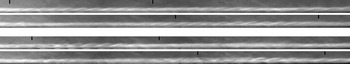
Figure 11. Image pairs (in each the separation is
 $31.7~{\rm\mu}\text{s}$
) showing the propagation and development of second-mode wavepackets. The markers show the approximate extent of the wavepacket in the first image in each case and has been translated downstream in the second image according to the mean phase speed.
$31.7~{\rm\mu}\text{s}$
) showing the propagation and development of second-mode wavepackets. The markers show the approximate extent of the wavepacket in the first image in each case and has been translated downstream in the second image according to the mean phase speed.
4.1 Wavepacket appearance
In figure 11 we show two image pairs from the condition-B porous experiment in each of which pair the propagation of a wavepacket is visible; the two images in each case are separated by
 $31.7~{\rm\mu}\text{s}$
. The images of the lower pair are zoomed-in versions of those at
$31.7~{\rm\mu}\text{s}$
. The images of the lower pair are zoomed-in versions of those at
 $t_{i}+155.8$
and
$t_{i}+155.8$
and
 $187.4~{\rm\mu}\text{ s}$
in figure 7. For brevity in the following discussion, we refer to the two images in the upper pair (pair 1) as 1 : 1 and 1 : 2, and those in the lower pair (pair 2) as 2 : 1 and 2 : 2. The wavepacket in pair 1 is at an earlier stage of development than that in pair 2: the structures in image 1 : 2 are similar to those of 2 : 1, and in 2 : 2 the structures are becoming chaotic and indistinct, i.e. the wavepacket is close to breaking down. In image 1 : 1, the disturbance exhibits the characteristic oblique ‘rope-like’ appearance noted earlier (and observed by other researchers) with the visible features lying mainly within the upper part of the boundary layer. Later, in image 1 : 2 (and also in 2 : 1), the peaks of the rope-like structures appear to fold over, creating a more interwoven appearance reminiscent of plaits or braids. In the centre of the wavepackets, these peaks extend above the visual edge of the boundary layer. For convenience, we refer hereinafter to wavepackets in this later stage of development as ‘plaited’ and those with oblique structures as in image 1 : 1 as ‘rope-like’, though this distinction is necessarily subjective to some extent. In image 2 : 2, even as the bulk of the wavepacket takes on a chaotic, turbulent appearance, some of the stronger regular structures are seen to persist in the centre of the disturbance. A similar persistence of the second-mode structures was observed in the pressure measurements of Casper et al. (Reference Casper, Beresh and Schneider2014), but in this earlier work the rope-like structures were observed at the extremes of the breaking down wavepacket, with the centre developing into turbulence. The rope-like and plaited stages were regularly observed in the evolution of wavepackets in both this and other sequences: in figure 5, for example, the disturbance at
$187.4~{\rm\mu}\text{ s}$
in figure 7. For brevity in the following discussion, we refer to the two images in the upper pair (pair 1) as 1 : 1 and 1 : 2, and those in the lower pair (pair 2) as 2 : 1 and 2 : 2. The wavepacket in pair 1 is at an earlier stage of development than that in pair 2: the structures in image 1 : 2 are similar to those of 2 : 1, and in 2 : 2 the structures are becoming chaotic and indistinct, i.e. the wavepacket is close to breaking down. In image 1 : 1, the disturbance exhibits the characteristic oblique ‘rope-like’ appearance noted earlier (and observed by other researchers) with the visible features lying mainly within the upper part of the boundary layer. Later, in image 1 : 2 (and also in 2 : 1), the peaks of the rope-like structures appear to fold over, creating a more interwoven appearance reminiscent of plaits or braids. In the centre of the wavepackets, these peaks extend above the visual edge of the boundary layer. For convenience, we refer hereinafter to wavepackets in this later stage of development as ‘plaited’ and those with oblique structures as in image 1 : 1 as ‘rope-like’, though this distinction is necessarily subjective to some extent. In image 2 : 2, even as the bulk of the wavepacket takes on a chaotic, turbulent appearance, some of the stronger regular structures are seen to persist in the centre of the disturbance. A similar persistence of the second-mode structures was observed in the pressure measurements of Casper et al. (Reference Casper, Beresh and Schneider2014), but in this earlier work the rope-like structures were observed at the extremes of the breaking down wavepacket, with the centre developing into turbulence. The rope-like and plaited stages were regularly observed in the evolution of wavepackets in both this and other sequences: in figure 5, for example, the disturbance at
 $t_{i}+28.1~{\rm\mu}\text{s}$
is rope-like, whereas that at
$t_{i}+28.1~{\rm\mu}\text{s}$
is rope-like, whereas that at
 $t_{i}+155.0~{\rm\mu}\text{s}$
has a more plaited appearance. In some cases no distinct plaited state could be discerned in the development, the wavepacket being rope-like in one image pair and already breaking down in the next. This may indicate that the plaited state is sometimes bypassed, or simply that it is short lived.
$t_{i}+155.0~{\rm\mu}\text{s}$
has a more plaited appearance. In some cases no distinct plaited state could be discerned in the development, the wavepacket being rope-like in one image pair and already breaking down in the next. This may indicate that the plaited state is sometimes bypassed, or simply that it is short lived.
We also observed that the visualized disturbance strength just prior to breakdown could vary significantly, though this could not be quantified in a meaningful way because of the lack of calibration of the schlieren set-up. While this might indicate that the disturbance amplitude at saturation was varying, an alternative (and we believe, more likely) explanation is that the spanwise extent, and thus the effective integrated path length, of the various wavepackets differed.

Figure 12. (a,b) Schlieren visualizations from a smooth-wall condition-A experiment showing two distinct wavepackets, the first (a) in a ‘rope-like’ state, the second (b) in a ‘plaited’ state; (c,d) the power spectral distributions versus wall-normal distance of these two wavepackets (a
 $\rightarrow$
c; b
$\rightarrow$
c; b
 $\rightarrow$
d).
$\rightarrow$
d).
4.2 Evolution of disturbance wall-normal distribution
In our earlier work (Laurence et al. Reference Laurence, Wagner and Hannemann2014), when the power spectrum of a second-mode disturbance was plotted at different heights above the cone surface, a distinctive double peak at the location of the fundamental frequency was noted, with local maxima both at the wall and inside the boundary layer. Such an example from a condition-A smooth-wall sequence is shown in figure 12 (upper visualization and left panel). Wavepackets showing such wall-normal distributions were seen regularly throughout this sequence and were primarily in a rope-like state. For disturbances that had evolved into a plaited state, however, the wall-normal distribution generally exhibited a subtle difference, as exemplified in the right panel of figure 12 (corresponding to the lower schlieren visualization). Here we see the development of a third peak close to the boundary-layer edge, with the remainder of the distribution remaining similar to that of the rope-like disturbance.
By examining the propagating wavepackets visualized in figure 11, we can gain further insight into the evolution of the wall-normal distribution. In figure 13 we show the distributions derived from the four images associated with the upper pair of figure 11 (i.e. the first and third distributions here correspond to images 1 : 1 and 2 : 1); in figure 14 the same is done with the four images associated with the lower pair of figure 11. The first distribution of figure 13(a) shows the double-peaked profile characteristic of the rope-like state, but already a slight relative growth in the region near the boundary-layer edge is visible. This continues in the subsequent image (b), with the strength of the third, near-edge peak now similar to that of the second peak at
 $y/{\it\delta}\approx 0.7$
. Growth in the near-wall part of the distribution is also apparent between the first two images, though this near-wall peak has almost vanished in the subsequent distribution (c). Redistribution of the disturbance energy towards the boundary-layer edge continues, but by the fourth image (d) the strength of the disturbance has waned and a spreading in frequency is also observed.
$y/{\it\delta}\approx 0.7$
. Growth in the near-wall part of the distribution is also apparent between the first two images, though this near-wall peak has almost vanished in the subsequent distribution (c). Redistribution of the disturbance energy towards the boundary-layer edge continues, but by the fourth image (d) the strength of the disturbance has waned and a spreading in frequency is also observed.

Figure 13. Development of the wall-normal power spectral distribution of the wavepacket shown in the upper image pair of figure 11: (a) corresponds to the first image in the pair; the subsequent distributions are at time lags relative to the first of (b) 4.5, (c) 31.7 and (d)
 $34.5~{\rm\mu}\text{s}$
.
$34.5~{\rm\mu}\text{s}$
.
In figure 14, we see a similar evolution in the outer part of the boundary layer in the first two distributions (a,b), with the splitting of the disturbance energy between the two outer peaks even more pronounced. In this case the near-wall peak is still present, which may indicate that the wavepacket in the sequence of figure 13 was displaced slightly in the circumferential direction from the vertical imaging plane, obscuring the near-wall peak in the later images. Harmonics of the second mode near 750 kHz are clearly visible in these upper two distributions; more shall be said about this in the following subsection. In the lower two panels (c,d), we see that the strength of the fundamental has decreased markedly across the boundary layer as the wavepacket undergoes breakdown, though the triple-peaked distribution is still distinguishable. In the lower left panel (c), an additional strong component has appeared at a value of
 $y/{\it\delta}$
lying between the two outer peaks, but at a slightly lower frequency: 310 kHz versus 380 kHz. This is interesting in light of the observation of Stetson & Kimmel (Reference Stetson and Kimmel1993) that spectral dispersion can occur just prior to breakdown; that is, as the second mode attenuates, neighbouring frequencies can experience rapid growth. This new component has itself been substantially attenuated in the final panel (figure 14
d). Finally, we note that the strength of the first harmonic is little changed between figures 14(b) and 14(c) despite the decay of the fundamental peaks.
$y/{\it\delta}$
lying between the two outer peaks, but at a slightly lower frequency: 310 kHz versus 380 kHz. This is interesting in light of the observation of Stetson & Kimmel (Reference Stetson and Kimmel1993) that spectral dispersion can occur just prior to breakdown; that is, as the second mode attenuates, neighbouring frequencies can experience rapid growth. This new component has itself been substantially attenuated in the final panel (figure 14
d). Finally, we note that the strength of the first harmonic is little changed between figures 14(b) and 14(c) despite the decay of the fundamental peaks.

Figure 14. Development of the wall-normal power spectral distribution of the wavepacket shown in the lower image pair of figure 11. (a) corresponds to the first image in the pair; the subsequent distributions are at time lags relative to the first of (b) 4.5, (c) 31.7, and (d)
 $34.5~{\rm\mu}\text{s}$
.
$34.5~{\rm\mu}\text{s}$
.
4.3 Harmonic development
In § 3, we saw that no harmonics were clearly discernible in the ensemble-averaged power spectra, whereas in the wall-normal distributions of figure 14, harmonic components are apparent at heights above the cone surface roughly coincident with the peaks in the fundamental. In examining the spectra of individual wave packets, harmonics were observed in some but not all cases, with plaited disturbances generally exhibiting stronger harmonics (as might be expected, given that they are at a later stage of development than rope-like waves). The development of nonlinear phenomena such as harmonics has been previously investigated using the bicoherence method (see, for example, Bountin, Shiplyuk & Maslov Reference Bountin, Shiplyuk and Maslov2008, Hofferth et al. Reference Hofferth, Humble, Floryan and Saric2013) - because of the lack of consistency in the appearance of harmonics in the present data, however, no such analysis was attempted here.

Figure 15. (a,d) Schlieren images of a propagating wavepacket in a smooth-surface condition-A sequence. The temporal separation of the images is
 $28~{\rm\mu}\text{s}$
, which corresponds to a propagation distance of 59 mm. Below each schlieren visualization are bandpass-filtered versions, with the filter centred around the second-mode fundamental frequency (b,e) and first harmonic frequency (c,f). (g) Power spectra at the
$28~{\rm\mu}\text{s}$
, which corresponds to a propagation distance of 59 mm. Below each schlieren visualization are bandpass-filtered versions, with the filter centred around the second-mode fundamental frequency (b,e) and first harmonic frequency (c,f). (g) Power spectra at the
 $y$
-location of maximum signal intensity for these two images: -▫- earlier; -▵- later. (h) Peak wall-normal distributions for the second-mode fundamental (-▫-) and first harmonic (-♢-) in the second of these two images. The relative magnitude of the harmonic has been multiplied by a factor of 2.25.
$y$
-location of maximum signal intensity for these two images: -▫- earlier; -▵- later. (h) Peak wall-normal distributions for the second-mode fundamental (-▫-) and first harmonic (-♢-) in the second of these two images. The relative magnitude of the harmonic has been multiplied by a factor of 2.25.
Some wavepackets were notable for the clarity of their harmonic content (this usually corresponded to high fundamental signal strength). In the images of figure 15, we show schlieren visualizations of one such propagating wavepacket from a condition-A smooth-surface sequence, together with processed versions that have been bandpass filtered around each of the fundamental and the first harmonic. For clarity, the amplitude of the first-harmonic-filtered image has been multiplied by a factor of 2.25 in comparison to the fundamental filtered image. In the earlier image the harmonic structures are only weakly visible near the centre of the wavepacket, but they become much more distinct in the later image. The angle formed by the harmonic structures to the cone surface is slightly steeper than that of the fundamental structures. The signal energy of both fundamental and harmonic components is more prominent in the upper half of the boundary layer, though there is also energy present near the surface. As noted in Laurence et al. (Reference Laurence, Wagner and Hannemann2014), the harmonic energy appears to be more concentrated towards the wavepacket centre in the streamwise direction than that of the fundamental.
In the lower left panel of figure 15, we show spectra from this wavepacket at both time instants, measured at
 $y/{\it\delta}=0.7$
(the height above the cone surface corresponding to maximum strength of the outer peak). Comparing to the spectra in the lower right panel of figure 6, we see the much higher signal strength relative to the noise floor that is obtained from considering a single wavepacket rather than the entire sequence. The fundamental and first harmonic peaks at 280 and 550 kHz are visible in each of the spectra, and we see substantial growth in both components as the wavepacket develops. In the downstream spectrum, there is an additional third peak close to where we would expect the second harmonic (820 kHz). To further elucidate the wall-normal distributions of these spectral components, in the lower right panel we show the peak strength of the fundamental and first harmonic versus the normalized wall-normal distance (note that no windowing has been applied to the spectra from which these are calculated, whereas in (g) a Blackman window has been employed). The harmonic also exhibits the double-peaked wall-normal profile we have noted of the fundamental for rope-like wavepackets. The outer peak of the harmonic here is centred closer to the wall than that of the fundamental; indeed, in all rope-like wavepackets examined, either the peaks were approximately coincident or the harmonic peak lay appreciably closer to the wall than the fundamental peak.
$y/{\it\delta}=0.7$
(the height above the cone surface corresponding to maximum strength of the outer peak). Comparing to the spectra in the lower right panel of figure 6, we see the much higher signal strength relative to the noise floor that is obtained from considering a single wavepacket rather than the entire sequence. The fundamental and first harmonic peaks at 280 and 550 kHz are visible in each of the spectra, and we see substantial growth in both components as the wavepacket develops. In the downstream spectrum, there is an additional third peak close to where we would expect the second harmonic (820 kHz). To further elucidate the wall-normal distributions of these spectral components, in the lower right panel we show the peak strength of the fundamental and first harmonic versus the normalized wall-normal distance (note that no windowing has been applied to the spectra from which these are calculated, whereas in (g) a Blackman window has been employed). The harmonic also exhibits the double-peaked wall-normal profile we have noted of the fundamental for rope-like wavepackets. The outer peak of the harmonic here is centred closer to the wall than that of the fundamental; indeed, in all rope-like wavepackets examined, either the peaks were approximately coincident or the harmonic peak lay appreciably closer to the wall than the fundamental peak.

Figure 16. (a,b) Bandpass-filtered versions of the lower image pair in figure 11, with the markers corresponding to the same locations; filters centred around the second-mode fundamental (upper image in each case) and first harmonic (lower image) have been applied. (c) Power spectra at the
 $y$
-location of maximum signal intensity for these two time instants: -▫- earlier; -
$y$
-location of maximum signal intensity for these two time instants: -▫- earlier; -
 $\triangle$
- later. (d) Peak wall-normal distributions for the second-mode fundamental (-▫-) and first harmonic (-♢-) for the first of these two images. The magnitude of the first harmonic has been multiplied by a factor of 5.
$\triangle$
- later. (d) Peak wall-normal distributions for the second-mode fundamental (-▫-) and first harmonic (-♢-) for the first of these two images. The magnitude of the first harmonic has been multiplied by a factor of 5.
In figure 16 we show equivalent results for the lower image pair of figure 11 (condition B); the markers are shown again for reference. In the bandpass-filtered versions of the first image, the oblique harmonic structures of the plaited wavepacket again coincide with those of the fundamental, both in location and roughly in angle. With the onset of breakdown in the second image, we can still make out the oblique fundamental structures in the centre and downstream (right of centre) part of the wavepacket, but the corresponding harmonic structures are visible over a more extended streamwise region, especially to the left of the wavepacket centre. This would help to explain the relatively strong harmonic component seen in the corresponding wall-normal distribution in figure 14(c).
By examining the structures in the fundamental filtered images of figures 15 and 16, we can also see the origin of the changes in the wall-normal distribution near the boundary-layer edge discussed in the previous subsection. When the wavepacket is in a rope-like state (figure 15), the dominant fundamental structures are simply the oblique features associated with the rope-like waves, which reach maximum strength above the midpoint of the boundary layer and then attenuate towards the outer edge. In a plaited wavepacket, on the other hand, although these oblique features persist near the centre of the wavepacket, the fundamental energy is now concentrated both at the peaks of these structures (which now extend above the boundary-layer height) and at a height where each individual wave structure folds over to intersect with the next in the packet. In between these two concentrations there is a relatively quiet zone, leading to a distribution with a split outer peak as seen in the upper panels of figure 14.
In the lower left-hand panel of figure 16 we show power spectra computed at
 $y/{\it\delta}=0.7$
for the wavepacket at these two time instants. As would be expected of a disturbance at the onset of breakdown, the strength of the fundamental has decreased substantially at the later instant; the first harmonic peak near 700 kHz, on the other hand, remains essentially unchanged and there is substantial growth in the part of the spectrum corresponding to the second harmonic (
$y/{\it\delta}=0.7$
for the wavepacket at these two time instants. As would be expected of a disturbance at the onset of breakdown, the strength of the fundamental has decreased substantially at the later instant; the first harmonic peak near 700 kHz, on the other hand, remains essentially unchanged and there is substantial growth in the part of the spectrum corresponding to the second harmonic (
 $f\gtrsim 1~\text{ MHz}$
). In the wall-normal distributions of the peak fundamental and first harmonic strengths in the earlier image of the pair (figure 16
d), we see that the first harmonic profile follows that of the fundamental relatively closely, with additional growth near the boundary-layer edge to form the triple-peaked distribution also characteristic of the fundamental in plaited wavepackets. As with the outer peak in rope-like disturbances, this third peak of the first harmonic was always observed to lie either close to the same
$f\gtrsim 1~\text{ MHz}$
). In the wall-normal distributions of the peak fundamental and first harmonic strengths in the earlier image of the pair (figure 16
d), we see that the first harmonic profile follows that of the fundamental relatively closely, with additional growth near the boundary-layer edge to form the triple-peaked distribution also characteristic of the fundamental in plaited wavepackets. As with the outer peak in rope-like disturbances, this third peak of the first harmonic was always observed to lie either close to the same
 $y/{\it\delta}$
as the corresponding fundamental peak, or more commonly, nearer to the wall. In a few cases the third peak was absent in the harmonic, though it was present in the fundamental.
$y/{\it\delta}$
as the corresponding fundamental peak, or more commonly, nearer to the wall. In a few cases the third peak was absent in the harmonic, though it was present in the fundamental.
4.4 Structure angle
Finally, we consider the ‘structure angle’ of the disturbances, i.e. the inclination of the line of constant phase in the
 $s$
–
$s$
–
 $y$
plane. Kimmel, Demetriades & Donaldson (Reference Kimmel, Demetriades and Donaldson1996) performed measurements of the structure angle in laminar and transitional hypersonic boundary layers using two hot-film probes. For the laminar cases, they found the angle to decrease slightly moving away from the surface, reaching a minimum value of approximately 15° at
$y$
plane. Kimmel, Demetriades & Donaldson (Reference Kimmel, Demetriades and Donaldson1996) performed measurements of the structure angle in laminar and transitional hypersonic boundary layers using two hot-film probes. For the laminar cases, they found the angle to decrease slightly moving away from the surface, reaching a minimum value of approximately 15° at
 $y/{\it\delta}=0.7$
, then increasing to 40–60° near the boundary-layer edge. Structure angles from limited schlieren visualizations were also reported by Laurence et al. (Reference Laurence, Wagner, Hannemann, Wartemann, Lüdeke, Tanno and Itoh2012), who observed the angle to decrease from 24° at
$y/{\it\delta}=0.7$
, then increasing to 40–60° near the boundary-layer edge. Structure angles from limited schlieren visualizations were also reported by Laurence et al. (Reference Laurence, Wagner, Hannemann, Wartemann, Lüdeke, Tanno and Itoh2012), who observed the angle to decrease from 24° at
 $y/{\it\delta}=0.4$
to 14–15° at
$y/{\it\delta}=0.4$
to 14–15° at
 $y/{\it\delta}=0.6$
–0.7; and by Parziale et al. (Reference Parziale, Shepherd and Hornung2015), who measured the angle of the main second mode structures near
$y/{\it\delta}=0.6$
–0.7; and by Parziale et al. (Reference Parziale, Shepherd and Hornung2015), who measured the angle of the main second mode structures near
 $y/{\it\delta}=0.6$
to be in the range of 11–15°.
$y/{\it\delta}=0.6$
to be in the range of 11–15°.
Here the structure angle,
 ${\it\theta}$
, was calculated by first bandpass filtering the image rows around the wavelength of interest (usually the second-mode fundamental), then calculating the cross-correlation coefficients for vertically separated rows at various relative streamwise displacements; the value of
${\it\theta}$
, was calculated by first bandpass filtering the image rows around the wavelength of interest (usually the second-mode fundamental), then calculating the cross-correlation coefficients for vertically separated rows at various relative streamwise displacements; the value of
 ${\it\theta}$
plotted here is the angle corresponding to the maximum of the resulting cross-correlation curves. In figure 17(a) we show the structure angles for the wavepacket in the two images of figure 15 (condition A, smooth surface); for the later image we show both the fundamental and first harmonic angles. For both images the fundamental angle,
${\it\theta}$
plotted here is the angle corresponding to the maximum of the resulting cross-correlation curves. In figure 17(a) we show the structure angles for the wavepacket in the two images of figure 15 (condition A, smooth surface); for the later image we show both the fundamental and first harmonic angles. For both images the fundamental angle,
 ${\it\theta}_{fund}$
, is 70–80°near
${\it\theta}_{fund}$
, is 70–80°near
 $y/{\it\delta}=0$
, then decreases away from the surface, at first rapidly but then more gently to reach a minimum of 12–13°;
$y/{\it\delta}=0$
, then decreases away from the surface, at first rapidly but then more gently to reach a minimum of 12–13°;
 ${\it\theta}_{fund}$
then increases sharply to
${\it\theta}_{fund}$
then increases sharply to
 ${\sim}100^{\circ }$
near the boundary-layer edge. The profile from the later image shows a kink at
${\sim}100^{\circ }$
near the boundary-layer edge. The profile from the later image shows a kink at
 $y/{\it\delta}$
=0.3 (where the fundamental strength is close to minimum), with
$y/{\it\delta}$
=0.3 (where the fundamental strength is close to minimum), with
 ${\it\theta}_{fund}$
increasing to
${\it\theta}_{fund}$
increasing to
 $50^{\circ }$
. The first harmonic structure angle,
$50^{\circ }$
. The first harmonic structure angle,
 ${\it\theta}_{harm}$
, shows generally similar behaviour to the fundamental, but with some differences: the angle is larger near the wall and the kink at
${\it\theta}_{harm}$
, shows generally similar behaviour to the fundamental, but with some differences: the angle is larger near the wall and the kink at
 $y/{\it\delta}$
=0.3 is more pronounced;
$y/{\it\delta}$
=0.3 is more pronounced;
 ${\it\theta}_{harm}$
also remains slightly larger near
${\it\theta}_{harm}$
also remains slightly larger near
 $y/{\it\delta}=0.7$
(consistent with our observations of figure 15), and the sharp rise in
$y/{\it\delta}=0.7$
(consistent with our observations of figure 15), and the sharp rise in
 ${\it\theta}$
near the boundary-layer edge occurs at smaller
${\it\theta}$
near the boundary-layer edge occurs at smaller
 $y/{\it\delta}$
. This latter point is consistent with our previous remarks regarding the tendency of the harmonic wall-normal distribution to be shifted slightly inwards relative to the fundamental distribution. The observations just made regarding the nature of the harmonic structure angle compared to the fundamental were found to generally hold over the disturbances examined in these sequences.
$y/{\it\delta}$
. This latter point is consistent with our previous remarks regarding the tendency of the harmonic wall-normal distribution to be shifted slightly inwards relative to the fundamental distribution. The observations just made regarding the nature of the harmonic structure angle compared to the fundamental were found to generally hold over the disturbances examined in these sequences.

Figure 17. Measured structure angle for the wavepackets seen in (a) figure 15 and (b) figure 12. (a) The curves correspond to: -▫-, the fundamental in the earlier image; -
 $\triangle$
-, the fundamental in the later image; and ——, the first harmonic in the later image. (b) The curves correspond to: ▫, the rope-like disturbance;
$\triangle$
-, the fundamental in the later image; and ——, the first harmonic in the later image. (b) The curves correspond to: ▫, the rope-like disturbance;
 $\triangle$
, the plaited disturbance.
$\triangle$
, the plaited disturbance.
To elucidate changes in the structure angle between rope-like and plaited disturbances, in figure 17(b) we show
 ${\it\theta}_{fund}$
for the two wavepackets of figure 12 (i.e. again condition A, smooth surface). We see in these disturbances that the kink at
${\it\theta}_{fund}$
for the two wavepackets of figure 12 (i.e. again condition A, smooth surface). We see in these disturbances that the kink at
 $y/{\it\delta}=0.3$
has grown to become a much more substantive feature, with the value of
$y/{\it\delta}=0.3$
has grown to become a much more substantive feature, with the value of
 ${\it\theta}_{fund}$
reaching 140° for the second (plaited) wave packet. For this more developed disturbance we also notice a slight rise in
${\it\theta}_{fund}$
reaching 140° for the second (plaited) wave packet. For this more developed disturbance we also notice a slight rise in
 ${\it\theta}_{fund}$
near
${\it\theta}_{fund}$
near
 $y/{\it\delta}=0.7$
(relative to the other cases examined thus far).
$y/{\it\delta}=0.7$
(relative to the other cases examined thus far).

In figure 18 we present the development of
 ${\it\theta}_{fund}$
for the two wavepackets of figures 13 and 14 (condition B, porous surface). For the first (figure 18
a), in the earlier stages of development the angle increases from 70–80° near the wall (i.e. the lines of constant phase are almost normal to the surface) to form a pronounced hump from
${\it\theta}_{fund}$
for the two wavepackets of figures 13 and 14 (condition B, porous surface). For the first (figure 18
a), in the earlier stages of development the angle increases from 70–80° near the wall (i.e. the lines of constant phase are almost normal to the surface) to form a pronounced hump from
 $y/{\it\delta}=0.2$
–0.4, peaking at
$y/{\it\delta}=0.2$
–0.4, peaking at
 ${\it\theta}=150{-}160^{\circ }$
. The curves thereafter follow a similar pattern to that seen previously. This hump is completely absent in the later two curves, but this is an anomalous case: all other plaited wavepackets examined - and some well-developed rope-like packets – exhibited this feature (see also figure 18
b). Its absence here might be linked to the apparent disappearance of the near-wall peak in the wall-normal distributions of figure 13(c,d). Other than this one atypical case, the general trend for this feature near
${\it\theta}=150{-}160^{\circ }$
. The curves thereafter follow a similar pattern to that seen previously. This hump is completely absent in the later two curves, but this is an anomalous case: all other plaited wavepackets examined - and some well-developed rope-like packets – exhibited this feature (see also figure 18
b). Its absence here might be linked to the apparent disappearance of the near-wall peak in the wall-normal distributions of figure 13(c,d). Other than this one atypical case, the general trend for this feature near
 $y/{\it\delta}=0.3$
is for it to grow in width and maximum value as the wavepacket evolves, reaching an angle as large as 160°. As this would involve the structures tilting forward at 20–30° to the upstream wall, this feature may be associated with the folding over of the wavepacket structures back towards the wall.
$y/{\it\delta}=0.3$
is for it to grow in width and maximum value as the wavepacket evolves, reaching an angle as large as 160°. As this would involve the structures tilting forward at 20–30° to the upstream wall, this feature may be associated with the folding over of the wavepacket structures back towards the wall.
In figure 18(b) we show the development of
 ${\it\theta}_{fund}$
for the wavepacket of figure 14. The rise near
${\it\theta}_{fund}$
for the wavepacket of figure 14. The rise near
 $y/{\it\delta}=0.7$
is now very pronounced in the earliest curve, but becomes progressively less so as the wavepacket develops further (the peak of the
$y/{\it\delta}=0.7$
is now very pronounced in the earliest curve, but becomes progressively less so as the wavepacket develops further (the peak of the
 $y/{\it\delta}=0.3$
feature decreasing simultaneously). A small rise was observed near this location for a number of plaited wavepackets, although none quite so pronounced as that seen here; this rise may also be related to the folding back of the wave structures, as this would tend to increase the apparent structure angle. The minimum value of
$y/{\it\delta}=0.3$
feature decreasing simultaneously). A small rise was observed near this location for a number of plaited wavepackets, although none quite so pronounced as that seen here; this rise may also be related to the folding back of the wave structures, as this would tend to increase the apparent structure angle. The minimum value of
 ${\it\theta}_{fund}$
for these curves is 8–9° which was the smallest value recorded amongst the wavepackets examined. Typically, the minimum angle lay in the range 10–14°.
${\it\theta}_{fund}$
for these curves is 8–9° which was the smallest value recorded amongst the wavepackets examined. Typically, the minimum angle lay in the range 10–14°.
5 High-enthalpy results
Two experiments were performed at the higher-enthalpy condition D of table 1; in both cases the visualizations were on the smooth side. In figure 19 we present a sequence of schlieren images from one of these experiments, illustrating the propagation and growth of a second-mode wavepacket in the cone boundary layer. Because of the low density of this condition, the second-mode disturbances were barely visible in the original images, even after contrast enhancement. Thus, to reveal the boundary-layer structures more clearly, all images in figure 19 have had a reference image (constructed by averaging 60 images within the sequence) subtracted before contrast enhancement was applied. The markers in the image at
 $t=20~{\rm\mu}\text{s}$
(fifth from top) indicate the approximate extent of the wavepacket at this point in its development; these have been displaced according to the mean phase velocity at all other time steps, revealing the streamwise spreading of the wavepacket as it propagates. Also notable in these images is the concentration of disturbance energy near the cone surface. In fact, in the early stages of its development, the wavepacket is visible only as a periodic pattern of light and dark regions at the wall, without any visible structures penetrating into the boundary layer. This is quite different from the appearance of disturbances in images obtained at the low-enthalpy conditions presented earlier; more will be said about this shortly.
$t=20~{\rm\mu}\text{s}$
(fifth from top) indicate the approximate extent of the wavepacket at this point in its development; these have been displaced according to the mean phase velocity at all other time steps, revealing the streamwise spreading of the wavepacket as it propagates. Also notable in these images is the concentration of disturbance energy near the cone surface. In fact, in the early stages of its development, the wavepacket is visible only as a periodic pattern of light and dark regions at the wall, without any visible structures penetrating into the boundary layer. This is quite different from the appearance of disturbances in images obtained at the low-enthalpy conditions presented earlier; more will be said about this shortly.

Figure 19. Sequence of reference subtracted schlieren images showing the propagation and growth of a wavepacket in a high-enthalpy boundary layer,
 $s=742{-}912~\text{mm}$
.
$s=742{-}912~\text{mm}$
.

Figure 20. (a,b) Time-developing power spectra just above the cone surface for the visualization regions (a)
 $s=750{-}830~\text{mm}$
and (b)
$s=750{-}830~\text{mm}$
and (b)
 $s=830{-}910~\text{mm}$
in figure 19. The broadband feature at
$s=830{-}910~\text{mm}$
in figure 19. The broadband feature at
 $2~\text{ms}$
in the downstream spectrum was caused by a piece of debris. (c,d) Mean power spectra for this experiment (c) along the cone surface and (d) at three discrete locations (-○-, 775 mm; -▫-, 825 mm; -▵-, 875 mm).
$2~\text{ms}$
in the downstream spectrum was caused by a piece of debris. (c,d) Mean power spectra for this experiment (c) along the cone surface and (d) at three discrete locations (-○-, 775 mm; -▫-, 825 mm; -▵-, 875 mm).
In the sequence exemplified in figure 19, a total of 44 correlated image pairs with wavepackets were identified, from which a mean phase speed of
 $3681\pm 145~\text{m}~\text{s}^{-1}$
(95 % confidence interval) was determined. For the second high-enthalpy sequence, the calculated phase speed was
$3681\pm 145~\text{m}~\text{s}^{-1}$
(95 % confidence interval) was determined. For the second high-enthalpy sequence, the calculated phase speed was
 $3807\pm 160~\text{m}~\text{s}^{-1}$
; considering the measurement uncertainty and shot-to-shot variation, this can be considered good agreement. Again, assuming the edge velocity to correspond to the Taylor–MacColl solution at the surface, these values indicate a propagation speed of 85–88 % of the edge velocity. In figure 20(a,b) we show time-resolved power spectra just above the cone surface for the upstream and downstream sections of the visualization window. The quasi-steady test period here is approximately 1.9 to
$3807\pm 160~\text{m}~\text{s}^{-1}$
; considering the measurement uncertainty and shot-to-shot variation, this can be considered good agreement. Again, assuming the edge velocity to correspond to the Taylor–MacColl solution at the surface, these values indicate a propagation speed of 85–88 % of the edge velocity. In figure 20(a,b) we show time-resolved power spectra just above the cone surface for the upstream and downstream sections of the visualization window. The quasi-steady test period here is approximately 1.9 to
 $2.7~\text{ms}$
. Throughout the plotted duration, the intermittent peaks centred between 500 and 700 kHz reveal the passage of second-mode disturbances across the visualization window; during the test time, the disturbance frequencies are concentrated around
$2.7~\text{ms}$
. Throughout the plotted duration, the intermittent peaks centred between 500 and 700 kHz reveal the passage of second-mode disturbances across the visualization window; during the test time, the disturbance frequencies are concentrated around
 $600~\text{kHz}$
. The signal strength is notably greater in the downstream section. The disturbance shown in figure 19 corresponds to the first of the two prominent peaks at
$600~\text{kHz}$
. The signal strength is notably greater in the downstream section. The disturbance shown in figure 19 corresponds to the first of the two prominent peaks at
 $t\approx 2.4~\text{ms}$
(note that the broadband streak just before
$t\approx 2.4~\text{ms}$
(note that the broadband streak just before
 $2~\text{ms}$
was caused by the passage of a piece of debris across the boundary layer and is not physically meaningful). Following the conclusion of the test time, the wavepackets become less frequent and show a trend towards lower frequencies: this is related to the decreasing Reynolds number caused by the drop in reservoir pressure and/or possible driver-gas contamination.
$2~\text{ms}$
was caused by the passage of a piece of debris across the boundary layer and is not physically meaningful). Following the conclusion of the test time, the wavepackets become less frequent and show a trend towards lower frequencies: this is related to the decreasing Reynolds number caused by the drop in reservoir pressure and/or possible driver-gas contamination.
In the lower panels of figure 20 we show the spatial development of the spectrum at the cone surface, continuously in (c) and at three discrete locations in (d). On the former we have added lines corresponding to the peak fundamental strength as a function of distance downstream (black dashed), as well as the approximate neutral stability boundaries calculated from the spectra (white dashed). In both panels we see strong growth of the fundamental peak at
 $600~\text{kHz}$
across the entire region considered. Only a slight decrease in the peak frequency is observed; note that these measurements are performed further downstream than those described in previous sections, and thus the rate of boundary-layer growth will be smaller. In the right lower panel, the ratio of the second-mode peak strength to the noise floor level is significantly higher than in the earlier measurements described in § 3, but still only very weak evidence of the first harmonic at
$600~\text{kHz}$
across the entire region considered. Only a slight decrease in the peak frequency is observed; note that these measurements are performed further downstream than those described in previous sections, and thus the rate of boundary-layer growth will be smaller. In the right lower panel, the ratio of the second-mode peak strength to the noise floor level is significantly higher than in the earlier measurements described in § 3, but still only very weak evidence of the first harmonic at
 $1200~\text{kHz}$
is visible.
$1200~\text{kHz}$
is visible.

Figure 21. Power spectra at the cone surface for the wavepacket shown in figure 19 at times
 $t=0$
(-○-), 10 (-▫-), 20 (-▵-), and
$t=0$
(-○-), 10 (-▫-), 20 (-▵-), and
 $30~{\rm\mu}\text{s}$
(-♢-). The approximate
$30~{\rm\mu}\text{s}$
(-♢-). The approximate
 $s$
-values on the cone surface corresponding to these times are 778, 814, 851 and 888 mm.
$s$
-values on the cone surface corresponding to these times are 778, 814, 851 and 888 mm.
Concentrating now on the individual wavepacket seen propagating in figure 19, in figure 21 we show the power spectrum at several points in its evolution, spanning a time of
 $30~{\rm\mu}\text{s}$
and a propagation distance of 110 mm. Growth and frequency shifting of the fundamental peak are clearly apparent, but now we also see a similar trend in the development of the first harmonic, together with the appearance of the second harmonic close to
$30~{\rm\mu}\text{s}$
and a propagation distance of 110 mm. Growth and frequency shifting of the fundamental peak are clearly apparent, but now we also see a similar trend in the development of the first harmonic, together with the appearance of the second harmonic close to
 $1700~\text{kHz}$
in the last spectrum (and possibly in earlier spectra). The ratio of strengths of the fundamental and first harmonic peaks in the later spectra is almost two orders of magnitude – much larger than in the equivalent low-enthalpy spectra in figures 15 and 16 (which is not surprising, considering we are further from transition here). Nevertheless, the harmonics are still easily discernible above the noise floor.
$1700~\text{kHz}$
in the last spectrum (and possibly in earlier spectra). The ratio of strengths of the fundamental and first harmonic peaks in the later spectra is almost two orders of magnitude – much larger than in the equivalent low-enthalpy spectra in figures 15 and 16 (which is not surprising, considering we are further from transition here). Nevertheless, the harmonics are still easily discernible above the noise floor.

Figure 22. Image intensity data along the cone surface for two propagating wavepackets, bandpass filtered around the second-mode fundamental (lighter) and first harmonic (darker), the latter multiplied by a factor of two for clarity. The experimental times in each case are (top to bottom)
 $t=0$
, 10, 20 and
$t=0$
, 10, 20 and
 $30~{\rm\mu}\text{s}$
; the left panel is from the sequence seen in figure 19 (at the same time steps).
$30~{\rm\mu}\text{s}$
; the left panel is from the sequence seen in figure 19 (at the same time steps).
The bandpass-filtered versions of these high-enthalpy visualizations, as in figures 15 and 16, were not found to be particularly revealing. Instead, in figure 22 we show intensity data for a single row near the surface, filtered around both the fundamental and first harmonic, for two propagating wavepackets (the left panel corresponds to the disturbance of figure 19). Temporal succession is indicated by downward vertical displacement, with a separation of
 $10~{\rm\mu}\text{s}$
between each profile. Each wavepacket shows steady growth in amplitude as it propagates downstream; in the left panel, we also see streamwise spreading of the disturbance envelope. Little spreading is evident in the wavepacket in the right panel, but at the last time step we do notice an interesting effect: the disturbance envelope has developed a V-shaped kink near 880 mm, rather than smoothly increasing then decreasing. A similar phenomenon was observed during the nonlinear development of a wavepacket in the DNS study of Sivasubramanian & Fasel (Reference Sivasubramanian and Fasel2014). At the earlier time steps it is difficult to resolve the presence of the first harmonic above the noise, but significant harmonic oscillations become clearer at later times. These exhibit a rather irregular envelope in comparison to the fundamental.
$10~{\rm\mu}\text{s}$
between each profile. Each wavepacket shows steady growth in amplitude as it propagates downstream; in the left panel, we also see streamwise spreading of the disturbance envelope. Little spreading is evident in the wavepacket in the right panel, but at the last time step we do notice an interesting effect: the disturbance envelope has developed a V-shaped kink near 880 mm, rather than smoothly increasing then decreasing. A similar phenomenon was observed during the nonlinear development of a wavepacket in the DNS study of Sivasubramanian & Fasel (Reference Sivasubramanian and Fasel2014). At the earlier time steps it is difficult to resolve the presence of the first harmonic above the noise, but significant harmonic oscillations become clearer at later times. These exhibit a rather irregular envelope in comparison to the fundamental.


Finally, we return to the wall-normal distribution of the disturbance energy within the boundary layer at these conditions. In figure 23 we show power spectra at different heights,
 $y$
, above the cone surface for each of the wavepackets in figure 22 at
$y$
, above the cone surface for each of the wavepackets in figure 22 at
 $t=30~{\rm\mu}\text{s}$
(a) and
$t=30~{\rm\mu}\text{s}$
(a) and
 $20~{\rm\mu}\text{s}$
(b). No effort was made to determine the boundary-layer height at these conditions because of the large expected departure from perfect gas behaviour. Similar to the distributions of the low-enthalpy rope-like wavepackets, in both cases we see a local maximum of the second-mode fundamental away from the cone surface, with the disturbance intensity dropping off for larger
$20~{\rm\mu}\text{s}$
(b). No effort was made to determine the boundary-layer height at these conditions because of the large expected departure from perfect gas behaviour. Similar to the distributions of the low-enthalpy rope-like wavepackets, in both cases we see a local maximum of the second-mode fundamental away from the cone surface, with the disturbance intensity dropping off for larger
 $y$
. The signal magnitude at the wall, however, is much larger than anywhere else inside the boundary layer; in both distributions it is approximately three times the other local (outer) maximum. This was consistently observed of wavepackets in the high-enthalpy experiments and is a significant point of difference to the low-enthalpy wavepackets, which exhibited a more balanced distribution of signal energy between peaks. We have noted in § 2.3 that caution is necessary when quantitatively comparing the near-wall signal magnitude with that elsewhere in the boundary layer; nevertheless, the scale of the discrepancy between low- and high-enthalpy distributions observed here suggests it to be physical meaningful.
$y$
. The signal magnitude at the wall, however, is much larger than anywhere else inside the boundary layer; in both distributions it is approximately three times the other local (outer) maximum. This was consistently observed of wavepackets in the high-enthalpy experiments and is a significant point of difference to the low-enthalpy wavepackets, which exhibited a more balanced distribution of signal energy between peaks. We have noted in § 2.3 that caution is necessary when quantitatively comparing the near-wall signal magnitude with that elsewhere in the boundary layer; nevertheless, the scale of the discrepancy between low- and high-enthalpy distributions observed here suggests it to be physical meaningful.
6 Discussion and conclusions
We begin our discussion by summarizing the phenomena observed during the evolution of wavepackets under low-enthalpy conditions up to incipient breakdown. Initially the waves exhibit a rope-like appearance with the fundamental structure angle decreasing from
 ${\sim}90^{\circ }$
near the wall to 10–14° at
${\sim}90^{\circ }$
near the wall to 10–14° at
 $y/{\it\delta}\approx 0.8$
. The fundamental energy has two local maxima of roughly equal strength: one at the wall and an outer peak at
$y/{\it\delta}\approx 0.8$
. The fundamental energy has two local maxima of roughly equal strength: one at the wall and an outer peak at
 $y/{\it\delta}\approx 0.7$
–0.75. As nonlinear processes become significant within the disturbance, indicated by the appearance of harmonics, the first (strongest) harmonic exhibits a structure angle slightly larger than the fundamental; it also shows a similar two-peaked distribution in energy, but shifted slightly towards the wall in comparison to the fundamental distribution. As the wavepacket evolves further and approaches breakdown, it takes on a plaited appearance with the wave structures folding over and becoming increasingly interwoven. This coincides with an increase in disturbance strength (both the fundamental and harmonic) just beyond the outer edge of the boundary layer and saturation of the disturbance energy further inside, a development that bears a superficial resemblance to the discredited transition onset model of Fischer & Weinstein (Reference Fischer and Weinstein1972). Meanwhile, in the region between the two original maxima (
$y/{\it\delta}\approx 0.7$
–0.75. As nonlinear processes become significant within the disturbance, indicated by the appearance of harmonics, the first (strongest) harmonic exhibits a structure angle slightly larger than the fundamental; it also shows a similar two-peaked distribution in energy, but shifted slightly towards the wall in comparison to the fundamental distribution. As the wavepacket evolves further and approaches breakdown, it takes on a plaited appearance with the wave structures folding over and becoming increasingly interwoven. This coincides with an increase in disturbance strength (both the fundamental and harmonic) just beyond the outer edge of the boundary layer and saturation of the disturbance energy further inside, a development that bears a superficial resemblance to the discredited transition onset model of Fischer & Weinstein (Reference Fischer and Weinstein1972). Meanwhile, in the region between the two original maxima (
 $y/{\it\delta}=0.2$
–0.4), the fundamental structure angle has reached values up to 160° (i.e. pointing upstream) and subsequently the angle close to the
$y/{\it\delta}=0.2$
–0.4), the fundamental structure angle has reached values up to 160° (i.e. pointing upstream) and subsequently the angle close to the
 $y/{\it\delta}=0.7$
maximum increases as the folding over of the wave structures becomes more pronounced. The redistribution of energy towards the boundary-layer edge continues as the internal peaks attenuate; this is followed by a rapid decrease in second-mode strength across the boundary layer, though the two-dimensional structures persist even as the wavepacket begins to take on a chaotic, turbulent appearance. We should note that in these later stages of the wavepacket evolution, the structures will become increasingly three-dimensional (Casper et al.
Reference Casper, Beresh and Schneider2014) and the ability of the schlieren technique to resolve them will be compromised.
$y/{\it\delta}=0.7$
maximum increases as the folding over of the wave structures becomes more pronounced. The redistribution of energy towards the boundary-layer edge continues as the internal peaks attenuate; this is followed by a rapid decrease in second-mode strength across the boundary layer, though the two-dimensional structures persist even as the wavepacket begins to take on a chaotic, turbulent appearance. We should note that in these later stages of the wavepacket evolution, the structures will become increasingly three-dimensional (Casper et al.
Reference Casper, Beresh and Schneider2014) and the ability of the schlieren technique to resolve them will be compromised.
At high enthalpy, we have seen that the distribution of disturbance energy across the boundary layer is somewhat different to the low-enthalpy case, with a much more pronounced concentration near the wall. We believe this phenomenon to originate from the highly cooled nature of the wall at high-enthalpy conditions. In the numerical simulations of Sivasubramanian & Fasel (Reference Sivasubramanian and Fasel2014), for example, the edge-to-wall temperature ratio was
 $T_{e}/T_{w}=0.18$
(or in terms of the adiabatic wall enthalpy,
$T_{e}/T_{w}=0.18$
(or in terms of the adiabatic wall enthalpy,
 $h_{w}/h_{aw}=0.80$
), and the density disturbance is weak near the wall (figure 16). For the cool-wall conditions of Parziale et al. (Reference Parziale, Shepherd and Hornung2015), however, the strength of the density fluctuations near the wall (figure 1 and private communication) substantially exceeds that further away from the surface. In this latter work,
$h_{w}/h_{aw}=0.80$
), and the density disturbance is weak near the wall (figure 16). For the cool-wall conditions of Parziale et al. (Reference Parziale, Shepherd and Hornung2015), however, the strength of the density fluctuations near the wall (figure 1 and private communication) substantially exceeds that further away from the surface. In this latter work,
 $M_{e}=5.93$
and
$M_{e}=5.93$
and
 $T_{e}/T_{w}=3.4$
(
$T_{e}/T_{w}=3.4$
(
 $h_{w}/h_{aw}=0.05$
), values similar to the present high-enthalpy experiments (
$h_{w}/h_{aw}=0.05$
), values similar to the present high-enthalpy experiments (
 $T_{e}/T_{w}=4.4$
,
$T_{e}/T_{w}=4.4$
,
 $h_{w}/h_{aw}=0.03$
).
$h_{w}/h_{aw}=0.03$
).
The differing natures of wavepackets at low and high enthalpies as revealed in these experiments raises some interesting questions. In the present work, we were able to visualize the high-enthalpy disturbances as they became nonlinear (as demonstrated by the presence of harmonics) but not through to the point of breakdown. Given the substantially different disturbance-energy distributions within the boundary layer, one might expect that the wavepacket evolution during breakdown could be qualitatively different at high enthalpy from that described above. Also of interest is the role of the entropy layer in blunted configurations such as the present one. The computations of Lau (Reference Lau2008), for example, have shown that the entropy layer can have a significant effect on the boundary-layer profile close to the wall (see figure 6 of that work); we thus might expect nose bluntness to influence the stability of the boundary layer somewhat differently if the disturbance energy is concentrated near the wall as in the present high-enthalpy experiments (and thus, presumably, the overall development towards breakdown is governed by what occurs in this near-wall region).
A further point concerns the use of control mechanisms for second-mode dominated transition, specifically ultrasonically absorptive surfaces such as the ceramic material employed in the present work. As the disturbance energy is effectively absorbed at the surface by such materials, one might expect their effectiveness to be enhanced for disturbances where the energy is concentrated near the wall. This would imply increased effectiveness of these mechanisms at values of
 $T_{e}/T_{w}$
much above unity. Considering that the recent numerical work of Bitter & Shepherd (Reference Bitter and Shepherd2015) has shown the second mode to be important for edge Mach numbers as low as 2.5 for highly cooled walls, questions such as those raised here would appear to take on an increased relevance for high-speed flight.
$T_{e}/T_{w}$
much above unity. Considering that the recent numerical work of Bitter & Shepherd (Reference Bitter and Shepherd2015) has shown the second mode to be important for edge Mach numbers as low as 2.5 for highly cooled walls, questions such as those raised here would appear to take on an increased relevance for high-speed flight.
Acknowledgements
The authors wish to gratefully acknowledge the assistance of the HEG technical staff, particularly Jan Martinez Schramm and Ingo Schwendtke, in operating the wind tunnel and setting up the experimental apparatus in these experiments.
Appendix. Spatial versus temporal measurements of the second mode
Compared to other methods for measuring second-mode disturbances, the schlieren technique employed here is unusual in that it measures the disturbance intensity over a finite spatial interval at a specified instant in time, rather than measuring a time series at a specific location. For studying the spatial development of wavepackets, the latter approach is the preferable one and it is of interest to ask how the measurements might differ if the present approach is taken. If we assign the ‘location’ of the spatial measurement to be the centre of the wavepacket,
 $x_{c}$
(however we choose to define this), and compare to a time-series measurement taken at
$x_{c}$
(however we choose to define this), and compare to a time-series measurement taken at
 $x_{c}$
, we note that the spatial part of the signal downstream of the centre (
$x_{c}$
, we note that the spatial part of the signal downstream of the centre (
 $x>x_{c}$
) will have undergone additional growth in comparison to the instant at which it was at
$x>x_{c}$
) will have undergone additional growth in comparison to the instant at which it was at
 $x_{c}$
, whereas the part upstream will be weaker in comparison to when it arrives at
$x_{c}$
, whereas the part upstream will be weaker in comparison to when it arrives at
 $x_{c}$
. Because the wavepacket growth is exponential, however, the stronger contribution from the downstream part will more than compensate for the weaker upstream part; the spatial signal will thus be slightly stronger than the equivalent time signal, and we might also expect the measured wavelength to be slightly larger, since this will increase with the growing boundary-layer thickness downstream. The signal strengthening is not of concern, since we are only concerned with changes in amplitude, rather than absolute magnitudes. The change in wavelength, however, could be experimentally observable.
$x_{c}$
. Because the wavepacket growth is exponential, however, the stronger contribution from the downstream part will more than compensate for the weaker upstream part; the spatial signal will thus be slightly stronger than the equivalent time signal, and we might also expect the measured wavelength to be slightly larger, since this will increase with the growing boundary-layer thickness downstream. The signal strengthening is not of concern, since we are only concerned with changes in amplitude, rather than absolute magnitudes. The change in wavelength, however, could be experimentally observable.

Figure 24. Comparison of power spectra measured at a specific location downstream in two condition-B experiments using (-▵-) the present schlieren technique and (-▫-) schlieren deflectometry.
In figure 24 we compare a spectrum determined using the present methodology with one measured using the schlieren deflectometry technique described in Laurence et al. (Reference Laurence, Wagner and Hannemann2014); the measurements are made at the same downstream location with the same nominal condition (B) but in different experiments. The vertical axes have been scaled so that the second-mode peaks have equal amplitudes. We note, as predicted, that the present measurement gives a slightly lower frequency (i.e. a longer wavelength) than the deflectometry measurement, though the effect is small and could also be partly due to natural variability between experiments (though a similar effect was noted when schlieren measurements were compared to surface pressure measurements in figure 12 of Laurence et al. Reference Laurence, Wagner and Hannemann2014). There is also a higher level of background noise with the present method; this may be related to the use of an extended light source for the deflectometry measurement, and the resulting focussing effect that would effectively remove some of the free stream noise from the signal. Overall, however, we conclude that the use of spatially resolved measurements here is a reasonable surrogate for the temporal measurements provided by other techniques.


