


1. INTRODUCTION
The Kalman Filter (KF) is considered to be an optimal estimation of the dynamic state and parameters from noisy measurements, and it has been widely used in process state estimation of integrated navigation systems. Nevertheless, the fact that the KF highly depends on a priori knowledge of the dynamic model parameters and noise statistics (Sangsuk-Iam and Bullock, Reference Sangsuk-Iam and Bullock1990; Fang and Yang, Reference Fang and Yang2011) is a major drawback, and the KF will potentially lose the optimal estimation quality if the a priori knowledge is unknown or time-varying. Unfortunately, the correct a priori knowledge of model parameters and noise statistics depends on several factors such as the process dynamics, which are difficult to obtain in many practical applications. In addition, the statistics of the process and measurement noise may change with time in a dynamic process. All of them will lead to the degradation of the estimation accuracy or even the unexpected divergence of the filters (Zhou et al., Reference Zhou, Knedlik and Loffeld2010; Al-Shabi et al., Reference Al-Shabi, Gadsden and Habibi2012).
Adaptive Kalman filtering (AKF) (Myers and Tapley, Reference Myers and Tapley1976; Ding et al., Reference Ding, Wang, Rizos and Kinlyside2007; Sarkka and Nummenmaa, Reference Sarkka and Nummenmaa2009; Karasalo and Hu, Reference Karasalo and Hu2011) can estimate the statistical characteristics of the process and measurement noise, simultaneously estimating the dynamic state and error covariance. As a result, various kinds of AKF have been applied to state and parameters estimation in dynamic systems, and they are broadly classified into four categories: Bayesian, maximum likelihood methods, correlation and covariance matching (Mehra, Reference Mehra1972; Wang, Reference Wang2000; Odelson et al., Reference Odelson, Rajamani and Rawlings2006). In particular, adaptive filtering based on Maximum Likelihood Estimation (MLE) (Mehra, Reference Mehra1970; Mohamed and Schwarz, Reference Mohamed and Schwarz1999) can obtain the approximate values of the process and measurement noise covariance by constantly tuning the noise covariance matrices online. Requiring quite a long innovation covariance sequence to achieve a reliable estimation, MLE still has the problem that the estimated noise covariance cannot be adjusted immediately with the recent innovation sequences in spite of the improvement in the filter stability (Mehra, Reference Mehra1970).
AKF based on Maximum a Posteriori (MAP) estimation (Sage and Husa, Reference Sage and Husa1969b; Gao et al., Reference Gao, You and Katayama2012) is affiliated with the Bayesian approach, and the noise statistical characteristics are estimated or modified consistently with the changes of the innovation sequence in the MAP noise estimator. In addition, the well-known Sage-Husa adaptive Kalman filtering (Sage and Husa, Reference Sage and Husa1969a), which is widely used in the estimation fields with unknown noise statistics, is just based on the MAP estimation. However, the MAP noise estimator at present has been shown to give biased estimation of true covariance (Bavdekar et al., Reference Bavdekar, Deshpande and Patwardhan2011).
To solve the degradation of accuracy or the divergence of the filter in the integration navigation system, an AKF algorithm based on MAP estimation and one-step smoothing filtering is proposed in this paper. An unbiased recursive noise estimator where noise statistics are recursively estimated or modified with the changes of innovation sequences is derived. In order to improve the accuracy of estimation, the AKF utilises the one-step smoothing value to modify the KF; moreover, the innovation covariances within a fixed moving window are averaged to correct the MAP noise estimator. Since the integration of the Strapdown Inertial Navigation System (SINS) and Doppler Velocity Log (DVL) system is a common navigation installation for vessels (Zhang, Reference Zhang2013), the performance of the proposed AKF algorithm is evaluated in the integrated SINS/DVL system, compared with the MLE and the Sage-Husa adaptive filtering algorithms. Moreover, the proposed AKF algorithm is also used to process the real voyage data of a marine vehicle for testing the actual estimation accuracy of the filter, and a long endurance test is also carried out to investigate the stability of the proposed AKF algorithm over long application periods.
This paper is organised as follows. In Section 2, the MAP noise estimator is given. In Section 3, an adaptive Kalman filtering algorithm with unbiased recursive noise estimator is derived in detail. In Section 4, experiments and analysis on the integrated SINS/DVL navigation system are carried out to evaluate the performance of the AKF. The conclusions are presented in Section 5.
2. MAP NOISE ESTIMATOR
The dynamic system model is described by the following equations:
 $${\bi X}_k = {\bf \Phi} _{k - 1} {\bi X} _{k - 1} + {\bf \Gamma} _{k - 1} {\bi W}_{k - 1} $$
 $${\bi Z}_k = {\bi H}_k {\bi X}_k + {\bi V}_k $$
where Xk ∈ Rn, Zk ∈ Rm, Φk−1 ∈ Rn×n, Γk−1 ∈ Rn×p and Hk∈Rm×n. Both Wk−1 ∈ Rp and Vk∈Rm are assumed to be uncorrelated Gaussian white noise sequences with mean and covariance matrices
 $$\eqalign{ & E[{\bi W}_k ] = {\bi q}_k, \;C{\rm ov}[{\bi W}_k, \;{\bi W}_j ] = {\bi Q}_k \delta _{kj} \cr & E[{\bi V}_k ] = {\bi r}_k, \;C{\rm ov}[{\bi V}_k, \;{\bi V}_j ] = {\bi R}_k \delta _{kj} \cr & C{\rm ov}[{\bi W}_k, \;{\bi V}_j ] = 0} $$
where E[·] denotes the expectation, Cov[·] denotes the covariance, and δ kj denotes the Kronecker delta function.
It is noted that the first moments of the process and measurement noise are not “zero”, which means the process and measurement noises are biased. Generally, the biases in the process and measurement noise are treated as “new” state variables in the functional modelling phase and are estimated during the propagation of the filter utilizing the approach of augmenting the dimension of system states. For example, Hewitson and Wang (Reference Hewitson and Wang2010), and Knight et al. (Reference Knight, Wang and Rizos2010) implemented the outlier detection, identification and reliability theory on the basis of the augmented dimension approach in order to remove the biases or fault measurements or outliers. Meanwhile, Sage and Husa (Reference Sage and Husa1969a; Reference Sage and Husa1969b), Myers and Tapley (Reference Myers and Tapley1976), and Gao et al. (Reference Gao, You and Katayama2012) provide another approach to deal with the biased process and/or measurement noise by establishing the relevant statistical mean and covariance estimators according to some optimal or suboptimal estimation rules. These noise estimators can estimate the statistics of the biased noise directly and correct the unrealistic noise parameters during the propagation of the filter, cutting down the estimation errors caused by the biased noise. In this paper, we deal with estimation problems of the biased noise according to motivation behind the second method and make some efforts to obtain the MAP estimator of the biased process and measurement noise.
If a priori means and covariances of the process noise qk, Qk and measurement noise rk, Rk are constant but unknown or random, the MAP estimations of  ${\bi \hat q},{\kern 1pt} {\bi \hat Q},{\kern 1pt} {\bi \hat r},{\kern 1pt} {\bi \hat R}$ can be obtained by maximizing the a posteriori density function (Sage and Husa, Reference Sage and Husa1969a). The noise estimator based on MAP estimation in coupling form can be expressed as follows:
 $${\bf \Gamma} _k {\bi \hat q}_k = \displaystyle{1 \over k}\sum\limits_{\,j = 1}^k {[{\bi \hat X}_{\,j,k} - {\bf \Phi} _{\,j - 1} {\bi \hat X}_{\,j - 1,k} ]} $$
 $${\bf \Gamma} _k {\bi \hat Q}_k {\bf \Gamma} _k^T = \displaystyle{1 \over k}\sum\limits_{j = 1}^k {[{\bi \hat X}_{j,k} - {\bf \Phi} _{j - 1} {\bi \hat X}_{j - 1,k} - {\bf \Gamma} _{j - 1} {\bi q}][{\bi \hat X}_{j,k} - {\bf \Phi} _{j - 1,k} {\bi \hat X}_{j - 1,k} - {\bf \Gamma} _{j - 1} {\bi q}]^T} $$
 $${\bi \hat r}_k = \displaystyle{1 \over k}\sum\limits_{\,j = 1}^k {[{\bi Z}_j - {\bi H}_j {\bi \hat X}_{\,j,k} ]} $$
 $${\bi \hat R}_k = \displaystyle{1 \over k}\sum\limits_{j = 1}^k {[{\bi Z}_j - {\bi H}_j {\bi \hat X}_{j,k} - {\bi r}][{\bi Z}_j - {\bi H}_j {\bi \hat X}_{j,k} - {\bi r}]^T} $$
Notice that complicated multistep smoothing terms (e.g.  ${\bi \hat X}_{\,j,k}, \;{\bi \hat X}_{\,j - 1,k} $) appear in Equations (2a)–(2d), and all previous state vectors are smoothed repeatedly by the latest measurements at every instant. In theory, the MAP noise estimator above could optimally estimate the statistical characteristics of the process and measurement noise, and it could modify the KF when noise statistics are unknown or time variant. However, it is impossible to estimate these noise statistics by directly utilising the MAP estimator in practical operations, as the MAP noise estimator cannot be described in a recursive form, in view of Equations (2a)–(2b), and each previous state vector needs to be smoothed by the latest measurements at every instant, which results in the inefficiency of the algorithm.
3. ADAPTIVE KALMAN FILTERING
In this paper, an AKF algorithm is proposed to solve the problems above on the basis of the MAP estimation, and the proposed AKF is divided into two main parts: one is a suboptimal noise estimator that can estimate the noise statistics; and the other is an improved Kalman filter, which utilises the outputs of the noise estimator to correct the estimate results.
3.1. Suboptimal MAP Noise Estimator
The inefficiency of the MAP noise estimator is due to the complicated multistep smoothing terms in Equations (2a)–(2b), thus some simplifications are taken in order to obtain the recursive form. Additionally, it is convenient and efficient if the noise estimator updates recursively, because only the estimate value at the previous step k-1 and the latest filter parameters at step k are used in the recursive update process, which greatly simplifies the process and decreases the calculations.
First, the one-step smoothing value  ${\bi \hat X}_{\,j - 1,j} $ takes the place of the multistep smoothing term
  ${\bi \hat X}_{\,j - 1,k} $ in Equations (2a) and (2d), and then the estimate value
  ${\bi \hat X}_{\,j,j} $ replaces the term
  ${\bi \hat X}_{\,j,k} $ in Equations (2a)–(2d). After these simplifications, a suboptimal MAP noise estimator is obtained as follows.
 $${\bf \Gamma} _k {\bi \hat q}_k = \displaystyle{1 \over k}\sum\limits_{\,j = 1}^k {[{\bi \hat X}_{\,j,j} - {\bf \Phi} _{\,j - 1} {\bi \hat X}_{\,j - 1,j} ]} $$
 $${\bf \Gamma} _k {\bi \hat Q}_k {\bf \Gamma} _k^T = \displaystyle{1 \over k}\sum\limits_{j = 1}^k {[{\bi \hat X}_{j,j} - {\bf \Phi} _{j - 1} {\bi \hat X}_{j - 1,j} - {\bf \Gamma} _{j - 1} {\bi q}][{\bi \hat X}_{j,j} - {\bf \Phi} _{j - 1} {\bi \hat X}_{j - 1,j} - {\bf \Gamma} _{j - 1} {\bi q}]^T} $$
 $${\bi \hat r}_k = \displaystyle{1 \over k}\sum\limits_{\,j = 1}^k {[{\bi Z}_j - {\bi H}_j {\bi \hat X}_{\,j,j} ]} $$
 $${\bi \hat R}_k = \displaystyle{1 \over k}\sum\limits_{j = 1}^k {[{\bi Z}_j - {\bi H}_j {\bi \hat X}_{j,j} - {\bi r}][{\bi Z}_j - {\bi H}_j {\bi \hat X}_{j,j} - {\bi r}]^T} $$
In view of Equations (3a)–(3d), only the estimate value  ${\bi \hat X}_{\,j,j} $ and one-step smoothing value
  ${\bi \hat X}_{\,j - 1,j} (\,j = 1,\;2 \ldots k)$ need to be updated in the suboptimal MAP noise estimator. It is noted that
  ${\bi \hat X}_{\,j,j} $ can be obtained from the conventional KF, but
  ${\bi \hat X}_{\,j - 1,j} $ cannot, so our first task is to obtain the one-step smoothing value
  ${\bi \hat X}_{\,j - 1,j} $.
3.2. Improved Kalman Filter
The improved KF consists of two procedures: the former utilises the estimate value at step k-1 and the innovation at k to calculate the one-step smoothing gain matrix and its corresponding smoothing value, and the latter modifies the estimate value  ${\bi \hat X}_{k - 1,k - 1} $ with the one-step smoothing value
  ${\bi \hat X}_{k - 1,k} $. Finally both the estimate value and the one-step smoothing value are propagated recurrently in the improved KF.
3.2.1. One-step Smoothing Filter
Firstly, our task is to obtain the one-step smoothing value  ${\bi \hat X}_{k - 1,k} $, which is used for the propagation of the noise estimator. According to the fixed point smoothing algorithm (Gustafsson, Reference Gustafsson2000), the one-step smoothing filter is obtained by utilising the measurements at step k.
 $${\bi \bar X}_{k,k - 1} = {\bf \Phi} _{k - 1} {\bi \hat X}_{k - 1,k - 1} + {\bf \Gamma} _{k - 1} {\bi q}_{k - 1} $$
 $${\bi \bar \varepsilon} _k = {\bi Z}_k - {\bi H}_k {\bi \bar X}_{k,k - 1} - {\bi r}_k $$
 $${\bi P}_{k,k - 1} = {\bf \Phi} _{k - 1} {\bi P}_{k - 1} {\bf \Phi} _{k - 1}^T + {\bf \Gamma} _{k - 1} {\bi Q}_{k - 1} {\bf \Gamma} _{k - 1}^T $$
 $${\bi \bar K}_k = {\bi P}_{k - 1} {\bf \Phi} _{k - 1}^T {\bi H}_k^T ({\bi H}_k {\bi P}_{k,k - 1} {\bi H}_k^T + {\bi R}_k )^{ - 1} $$
 $${\bi \hat X}_{k - 1,k} = {\bi \hat X}_{k - 1,k - 1} + {\bi \bar K}_k {\bi \bar \varepsilon} _k $$
where  ${\bi \bar X}_{k,k - 1} $ denotes the a priori estimate value,
  ${\bi \bar \varepsilon} _k $ denotes the innovation, Pk,k−1 denotes the a priori estimate error covariance,
  ${\bi \bar K}_k $ denotes the gain matrix, which is different from the KF in form, and
  ${\bi \hat X}_{k - 1,k} $ denotes the one-step smoothing value of the one-step smoothing filter, respectively. Additionally, the derivation of the one-step smoothing filter in detail is presented by Gustafsson (Reference Gustafsson2000), which is not derived in this paper.
3.2.2. Modified Kalman Filter
From Equations (3a)–(3b), it is noted that the connection between  ${\bi \hat X}_{k,k} $ and
  ${\bi \hat X}_{k - 1,k} $ is important to estimate the process noise statistics qk and Qk; moreover, the connection is also important in forming a closed-loop propagation for the noise estimator. Hence, we need to establish the connection between
  ${\bi \hat X}_{k,k} $ and
  ${\bi \hat X}_{k - 1,k} $. Specifically, the one-step smoothing value
  ${\bi \hat X}_{k - 1,k} $ is used to modify the a priori estimate value
  ${\bi \hat X}_{k,k - 1} $ by replacing
  ${\bi \hat X}_{k - 1,k - 1} $, the estimate value at step k-1, in the KF. The modified KF can be written as
 $${\bi \hat X}_{k,k - 1} = {\bf \Phi} _{k - 1} {\bi \hat X}_{k - 1,k} + {\bf \Gamma} _{k - 1} {\bi q}_{k - 1} $$
 $${\bi \varepsilon} _k {\bi = Z}_k - {\bi H}_k {\bi \hat X}_{k,k - 1} - {\bi r}_k $$
 $${\bi K}_k = {\bi P}_{k,k - 1} {\bi H}_k^T ({\bi H}_k {\bi P}_{k,k - 1} {\bi H}_k^T + {\bi R}_k )^{ - 1} $$
 $${\bi \hat X}_{k,k} = {\bi \hat X}_{k,k - 1} + {\bi K}_k {\bi \varepsilon} _k $$
 $${\bi P}_k = ({\bi I} - {\bi K}_k {\bi H}_k ){\bi P}_{k,k - 1} $$
where  ${\bi \hat X}_{k,k - 1} $ denotes the a priori estimate value, εk denotes the innovation, Kk denotes the gain matrix, and
  ${\bi \hat X}_{k,k} $ denotes the estimate value of the modified KF. It is noted that Pk,k−1 is the same in Equations (4d) and (5c).
Note that the connection between  ${\bi \hat X}_{k,k} $ and
  ${\bi \hat X}_{k - 1,k - 1} $ is described by Equations (5a) and (5d). It is convenient to introduce
  ${\bi \hat X}_{k - 1,k} $ into Equation (5a) to calculate the a priori estimate value
  ${\bi \hat X}_{k,k - 1} $, since
  ${\bi \hat X}_{k - 1,k} $ has been obtained in Equation (4e); besides, the estimation accuracy may be improved because
  ${\bi \hat X}_{k - 1,k} $ has been already estimated by the measurements at step k in Equation (5a).
At this point, the expected recursive suboptimal MAP noise estimator is obtained through substituting Equations (4a)–(5e) into Equations (3a)–(3d), but our work has not been finished yet. After these simplifications and arrangements, the MAP estimator has lost its optimal estimation quality, and our next task is to guarantee the unbiased estimation of the suboptimal MAP noise estimator.
3.3. Unbiased Suboptimal MAP Noise Estimator
An unbiased estimation test on the suboptimal noise estimator is performed, in order to guarantee that the estimations for the noise statistical means and covariances are unbiased.
In view of Equations (5a) and (5d), the general term  ${\bi \hat X}_{\,j,j} - {\bf \Phi} _{\,j - 1} {\bi \hat X}_{\,j - 1,j} $ in Equation (3a) can be written as
 $${\bi \hat X}_{\,j,j} - {\bf \Phi} _{\,j - 1} {\bi \hat X}_{\,j - 1,j} = {\bi K}_j {\bi \varepsilon} _j + {\bf \Gamma} _{\,j - 1} {\bi q}_{\,j - 1} $$
 Similarly, from Equations (5a)–(5d), the term  ${\bi Z}_j - {\bi H}_j {\bi \hat X}_{\,j,j} $ in Equation (3c) can be represented as
 $$\eqalign{ & {\bi Z}_j - {\bi H}_j {\bi \hat X}_{\,j,j} = {\bi Z}_j - {\bi H}_j ({\bi \hat X}_{\,j,j - 1} + {\bi K}_j {\bi \varepsilon} _j ) \cr & = ({\bi I} - {\bi H}_j {\bi K}_j ){\bi \varepsilon} _j + {\bi r}_j} $$
Therefore, an equivalent expression of the suboptimal MAP noise estimator is obtained after rearranging Equations (3a)–(3d).
 $${\bf \Gamma} _k {\bi \hat q}_k = \displaystyle{1 \over k}\sum\limits_{\,j = 1}^k {[{\bi K}_j {\bi \varepsilon} _j + {\bf \Gamma} _{\,j - 1} {\bi \hat q}_{\,j - 1} ]} $$
 $${\bf \Gamma} _k {\bi \hat Q}_k {\bf \Gamma} _k^T = \displaystyle{1 \over k}\sum\limits_{j = 1}^k {[{\bi K}_j {\bi \varepsilon} _j {\bi \varepsilon} _j^T {\bi K}_j^T ]} $$
 $${\bi \hat r}_k = \displaystyle{1 \over k}\sum\limits_{\,j = 1}^k {[({\bi I} - {\bi H}_j {\bi K}_j ){\bi \varepsilon} _j + {\bi r}_j ]} $$
 $${\bi \hat R}_k = \displaystyle{1 \over k}\sum\limits_{j = 1}^k {[({\bi I} - {\bi H}_k {\bi K}_j ){\bi \varepsilon} _j {\bi \varepsilon} _j^T ({\bi I} - {\bi H}_j {\bi K}_j )^T ]} $$
Notice that the innovation εj and its covariance εjεjT are contained in the process and measurement noise estimator, as described by Equations (8a)–(8d), and we can obtain the following:
 $$\eqalign{ & {\bi \varepsilon} _j = {\bi Z}_j - {\bi H}_j {\bi \hat X}_{\,j,j - 1} - {\bi r}_j \cr & = {\bi H}_j {\bi \tilde X}_{\,j,j - 1} + ({\bi V}_j - {\bi r}_j )} $$
 $$\eqalign{ & {\bi K}_j {\bi \varepsilon} _j {\bi \varepsilon} _j^T {\bi K}_j^T = {\bi K}_j {\bi H}_j {\bi P} _{j,j - 1}^T \cr & = {\bi K}_j {\bi H}_j {\bi P}_{j,j - 1} = {\bi P}_{j,j - 1} - {\bi P}_j \cr & = {\bf \Phi} _{j - 1} {\bi P}_{j - 1} {\bf \Phi} _{j - 1}^T - {\bi P}_j + {\bf \Gamma} _{j - 1} {\bi Q}_{j - 1} {\bf \Gamma} _{j - 1}^T} $$
Additionally, the derivation of Equation (10) refers to Equations (A1)–(A3) in the Appendix. Then by taking the expectations of εj and εjεjT yields the following:
 $$E[{\bi \varepsilon} _j ] = 0$$
 $$E[{\bi \varepsilon} _j {\bi \varepsilon} _j^T ] = {\bi H}_j {\bi P}_{j,j - 1} {\bi H}_j^T + {\bi R}$$
Substitute Equations (9)–(12) into Equations (8a)–(8d), and then the expectations of the process noise mean and covariance can be expressed as
 $$E[{\bf \Gamma} _k {\bi \hat q}_k ] = E\left\{ {\displaystyle{1 \over k}\sum\limits_{\,j = 1}^k {[{\bi K}_j {\bi \varepsilon} _j + {\bf \Gamma} _{\,j - 1} {\bi q}_{\,j - 1} ]}} \right\} = {\bf \Gamma} {\bi q}$$
 $$\eqalign{ & E[{\bf \Gamma} _k {\bi \hat Q}_k {\bf \Gamma} _k^T ] = E\left[ {\displaystyle{1 \over k}\sum\limits_{j = 1}^k {{\bi K}_j {\bi \varepsilon} _j {\bi \varepsilon} _j^T {\bi K}_j^T}} \right] \cr & = E\left\{ {\displaystyle{1 \over k}\sum\limits_{j = 1}^k {[{\bf \Phi} _{j - 1} {\bi P}_{j - 1} {\bf \Phi} _{j - 1}^T - {\bi P}_j + {\bf \Gamma} _{j - 1} {\bi Q}_{j - 1} {\bf \Gamma} _{j - 1}^T ]}} \right\} \cr & = {\bf \Gamma} {\bi Q}{\bf \Gamma} ^T + E\left\{ {\displaystyle{1 \over k}\sum\limits_{j = 1}^k {[{\bf \Phi} _{j - 1} {\bi P}_{j - 1} {\bf \Phi} _{j - 1}^T - {\bi P}_j ]}} \right\}} $$
Equation (13) demonstrates that Equation (8a) is the unbiased estimation of the process noise statistical mean. The unbiased estimation of process noise statistical covariance is obtained by rearranging Equation (14), and it can be written as
 $${\bf \Gamma} _k {\bi \hat Q}_k {\bf \Gamma} _k^T = \displaystyle{1 \over k}\sum\limits_{\,j = 1}^k {[{\bi K}_j {\bi \varepsilon} _j {\bi \varepsilon} _j^T {\bi K}_j^T + {\bi P}_j - {\bf \Phi} _{\,j - 1} {\bi P}_{\,j - 1} {\bf \Phi} _{\,j - 1}^T ]} $$
Similarly, the unbiased measurement noise estimator is obtained. In particular, Equation (8c) represents the unbiased estimation of measurement noise mean and the unbiased estimation of the covariance can be expressed as (derivations are shown in the Appendix):
 $$\hat R_k = \displaystyle{1 \over k}\sum\limits_{\,j = 1}^k ( {\bi I} - {\bi H}_j {\bi K}_j )[{\bi \varepsilon} _j {\bi \varepsilon} _j^T ({\bi I} - {\bi H}_j {\bi K}_j )^T + {\bi H}_j {\bi P}_{\,j,j - 1} {\bi H}_j^T ]$$
Consequently, Equations (8a), (8c), (15) and (16) make up the unbiased suboptimal MAP noise estimator.
3.4. Time-varying Unbiased Noise Estimator
The derivations of the noise estimator above are based on the assumption that the noise statistics are unknown constants. However, the noise statistics are generally time varying or random in practical situations.
Consider the case that the noise statistics are time varying, an exponentially weighted fading memory method is introduced to increase the weights of the recent innovations (Gao et al., Reference Gao, You and Katayama2012). A time-varying noise estimator is obtained after the weighted factor τ k replaces the term 1/k in Equations (8a), (8c), (15) and (16). Therefore, its recursive decoupling form can be represented as
 $${\bi \hat q}_k = {\bi \hat q}_{k - 1} + \Xi _k \{ \tau _k [{\bi K}_k \varepsilon _k ]\} $$
 $${\bi \hat Q}_{k} = (1 - \tau _k ){\bi \hat Q}_{k - 1} + \Xi _k \{ \tau _k [{\bi K}_k {\bi \varepsilon} _k {\bi \varepsilon} _k^T {\bi K}_k^T + {\bi P}_k - {\bf \Phi} _{k - 1} {\bi P}_{k - 1} {\bf \Phi} _{k - 1}^T ]\} \Xi _k^T $$
 $${\bi \hat r}_k = {\bi \hat r}_{k - 1} + \tau _k [({\bi I} - {\bi H}_k {\bi K}_k ){\bi \varepsilon} _k ]$$
 $${\bi \hat R =} (1 - \tau _k ){\bi \hat R}_{k - 1} + \tau _k ({\bi I} - {\bi H}_k {\bi K}_k )[{\bi \varepsilon} _k {\bi \varepsilon} _k^T ({\bi I} - {\bi H}_k {\bi K}_k )^T + {\bi H}_k {\bi P}_{k,k - 1} {\bi H}_k^T ]$$
where  ${\rm \Xi} _k = ({\bf \Gamma} _k^T {\bf \Gamma} _k )^{ - 1} {\bf \Gamma} _k^T, \;\tau _k = (1 - b)/(1 - b^k )$, and b is a fading factor, 0<b<1.
Equations (17a)–(17d) compose the unbiased recursive noise estimator that can provide accurate noise statistical parameters for the improved KF. However,  ${\bi \hat Q}_k $ and/or
  ${\bi \hat R}_k $ may be increased when applied to long application periods. The reason is that the estimation error of
  ${\bi \hat Q}_k $ and/or
  ${\bi \hat R}_k $, which is caused by a sudden measurement jump or outlier, will accumulate with the propagation of the recursive noise estimator. For this case, we should choose a small value of b to decrease the weights of the incorrect estimations in the recursive noise estimator and generally we choose a value below 0·2 in practice.
Additionally, in the KF, the covariance of the process noise  ${\bi \hat Q}_k $ is required to be a non-negative definite matrix and the covariance of the measurement noise
  ${\bi \hat R}_k $ to be a positive definite matrix in order to guarantee the stability of the filter. Since we obtain these noise estimators from the KF and one-step smoothing filter without any extra assumptions, in theory, the estimator
  ${\bi \hat Q}_k $ is a non-negative definite matrix from Equations (12), (14) and (17b), and
  ${\bi \hat R}_k $ is a positive definite matrix from Equations (5e), (12), (17d) and (A7). However, in view of Equations (17b) and (17d), the propagation of
  ${\bi \hat Q}_k $ and
  ${\bi \hat R}_k $ depends on the actual covariance εkεkT of the innovation sequence instead of its theoretical covariance. The covariance estimator
  ${\bi \hat Q}_k $ or
  ${\bi \hat R}_k $ may be likely to lose its non-negative definite or positive definite quality if a measurement outlier occurs unexpectedly during its recursive procedure in practice. Thus, we introduce an innovation covariance estimator to depress the estimation errors caused by the measurement outlier in Section 3.5.
3.5. Innovation Covariance Estimator
In view of Equations (17b) and (17d), there are complicated matrix iteration operations on  ${\bi \hat Q}_k $ and
  ${\bi \hat R}_k $; moreover, the innovation covariance εkεkT is relied on for the propagation of the noise estimator. When applied to long application periods,
  ${\bi \hat Q}_k $ and/or
  ${\bi \hat R}_k $ may be increased, which is caused by a sudden measurement jump or outlier and degrades the performance of the filter. Besides, it may even lead the AKF to divergence if some “bad” outliers from the innovation sequences occur during the propagation. In order to identify and remove the faulty measurements or outliers, some other procedures have been proposed in the past decade. For example, an outlier test based on the reliability theory is implemented by Knight et al. (Reference Knight, Wang and Rizos2010) to deal with the measurement outliers. More detailed information can be found in Hewitson and Wang (Reference Hewitson and Wang2006, Reference Hewitson and Wang2010).
To solve this problem, we can also utilise the discrepancy between the actual covariance and theoretical covariance of the innovation sequence. In this section, an innovation covariance estimator (ICE) (Jwo and Weng, Reference Jwo and Weng2008) is introduced for guaranteeing the non-negative definite or positive definite quality of  ${\bi \hat Q}_k $ or
  ${\bi \hat R}_k $. It estimates the innovation covariance online, through averaging the recent N-step innovation covariances. The ICE can be written as
 $${\bi C}_k = \displaystyle{1 \over N}\sum\limits_{\,j = 0}^{N - 1} {[{\bi \varepsilon}_{k - 1}^{} {\bi \varepsilon}_{k - j}^T ] = {\bi C}_{k - 1}^{} + \displaystyle{1 \over N}[{\bi \varepsilon} _k {\bi \varepsilon} _k^T - {\bi \varepsilon} _{k - N} {\bi \varepsilon} _{k - N}^T ]} $$
where N denotes the length of the moving window.
Then the ICE modifies the noise estimator by substituting the term εkεkT in Equations (17b) and (17d). Besides, the effect of the ICE on correcting the calculation of εkεkT contaminated by the measurement outlier is evident through averaging the recent N-step innovation covariances in practical applications.
In view of Equation (18), it is noted that the estimation accuracy of the innovation covariance estimators relies on the adjustments of the window size N. However, the proper choice of N highly depends on the dynamic characteristics of the system and the motion methods of the vehicle, and usually it is established by empirical knowledge. For details, consider a case of high-frequency changes of the trajectory; N needs to be a small value to adjust to the fast changes though the innovation covariance estimator will be biased. On the other hand, N needs to be a larger value to improve the stability and unbiased quality of the innovation covariance estimation when the system dynamics change slowly.
Furthermore, the discrepancy between ICE and theoretical covariance of the innovation sequence can be used for identifying the measurement outliers and evaluating the stability of the noise estimators. When the noise estimators are in stable status, the inequality satisfies
 $${\rm tr(}C_k ) \leqslant \kappa \cdot {\rm tr}({\bi H}_k {\bi P}_{k,k - 1} {\bi H}_k^T + {\bi R}_k )$$
where κ is a reserve factor, κ ⩾1, and κ is set up from the empirical knowledge; tr(·) is the trace operation on a matrix.
Actually, κ is a threshold value that reflects whether the noise estimators are in stable status or not. It indicates that the estimates of the noise statistics are incorrect and that the measurement outliers occur if the ratio between tr(Ck) and tr(HkPk,k −1HkT+Rk) is beyond the threshold value κ at current step. Therefore, the current innovation covariance εkεkT will be isolated from the calculation of the ICE for keeping the ICE robust and keeping the noise estimator  ${\bi \hat Q}_k $ and
  ${\bi \hat R}_k $ stable when the measurement outliers occur.
In view of Equations (4a)–(5e) and Equations (17a)–(17d), a complete adaptive Kalman filer is obtained. The AKF contains two segments: the former is the improved KF that utilises the innovation at step k to smooth the estimate value at step k-1, and then uses the one-step smoothing value to correct estimate results of the KF; the latter is the noise estimator that estimates or modifies the noise statistics with the innovation sequences to provide accurate statistics for the improved KF.
The operation of the adaptive Kalman filtering is represented as shown in Figure 1.
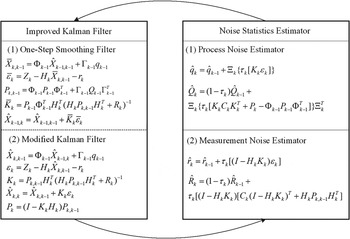
Figure 1. Operation of the adaptive Kalman filtering.
4. EXPERIMENT RESULTS AND ANALYSIS IN THE INTEGRATED SINS/DVL SYSTEM
To evaluate the performance of the proposed AKF in a dynamic system with unknown and time-varying measurement noise statistics, simulations in the integrated SINS/DVL system are performed firstly, and then real voyage data are also processed using the proposed AKF offline.
4.1. Simulation and Analysis in the SINS/DVL System
The SINS/DVL is integrated by a loosely coupled method and the diagram of the integration navigation system is shown in Figure 2. DVL velocity information is used to compensate SINS navigation errors through the adaptive Kalman filter, in which the navigation information from the subsystem is fused adaptively. Moreover, the output correction is applied to correct the navigation parameters from the SINS for navigation solutions.

Figure 2. Diagram of the integrated SINS/DVL navigation system.
The components of the position and velocity errors at a level plane are only considered in this paper as the vertical motion is negligible when a marine vehicle is sailing. Hence, the state vector x is composed of seven navigation error variables, and it is expressed as x=[δL δλ δν e δν n φ e φ n φ u]T. The state space model of the SINS that is a time varying linear stochastic system is described in Equation (20).
 $${\bi \dot x}({\rm t}) = {\bi Ax}({\rm t}) + {\bi Bw}({\rm t})$$
where w(t)=[0 0 w ax w ay w gx w gy w gz]T, and subscripts e, n, u denote the east, north and up components in the navigation frame, respectively, and x, y, z denote the right, front and up components in the body frame, respectively. The process noise vector w(t) consists of the Gaussian white noises of the accelerometers and gyroscopes. A is the state transition matrix and B is the process noise matrix. Besides, the elements of matrix A and B are listed as follows.
 $$\hskip-2\eqalign{ & {\bi A} = \left[ \matrix{\matrix{ {{\bi A}_{11}} & {{\bi A}_{12}} & {{\bi A}_{13}} \cr} \cr \matrix{ {{\bi A}_{21}} & {{\bi A}_{22}} & {{\bi A}_{23}} \cr} } \right], \ {\bi B =} \left[ {\matrix{ {{\bi B}_{11}} & {{\bf 0}_{4 \times 3}} \cr {{\bf 0}_{3 \times 4}} & {{\bi B}_{22}} \cr}} \right] \cr & {\bi A}_{11} = \left[ {\matrix{ 0 & 0 \cr {\displaystyle{{v_e} \over {R_n}} \ {\rm sec} \ L\tan L} & 0 \cr {2w_{ie} v_n \cos L + \displaystyle{{v_e v_n} \over {R_n}} {\rm sec}^2 L} & 0 \cr { - \left( {2w_{ie} v_n \cos L + \displaystyle{{v_e^2} \over {R_n}} {\rm sec}^2 L} \right)} & 0 \cr}} \right]\hskip-1 , \;\,\hskip-2 {\bi A}_{12} = \hskip-2 \left[ {\matrix{ {\displaystyle{1 \over {R_m}}} & 0 \cr {\displaystyle{{{\rm sec} \ L} \over {R_n}}} & 0 \cr {\displaystyle{{v_n} \over {R_n}} \tan L} & {2w_{ie} \sin L + \displaystyle{{v_e} \over {R_n}} \tan L} \cr { - \left( 2w_{ie} \sin L + \displaystyle{{v_e} \over {R_n}} \tan L \right)} & 0 } \cr}} \right] \cr & {\bi A}_{13} = \left[ \matrix{\matrix{ 0 & 0 & 0 \cr 0 & 0 & 0 \cr 0 & { - g} & {\,f_n} \cr} \cr \matrix{ g & 0 & { - f_e} \cr} } \right],\;{\bi A}_{21} = \left[ {\matrix{ 0 & 0 \cr { - w_{ie} \ {\rm sin} \, L} & 0 \cr {w_{ie} \cos L + {\displaystyle{{v_e} \over {R_n}}} \sec ^2 L} & 0 \cr}} \right]{\bi A}_{22} = \left[ {\matrix{ 0 & { - {\displaystyle{1 \over {R_m}}}} \cr {{\displaystyle{1 \over {R_n}}}} & 0 \cr {{\displaystyle{1 \over {R_n}}} \tan L} & 0 \cr}} \right] \cr & {\bi A}_{23} = \left[ {\matrix{ 0 & {w_{ie} \sin L + \displaystyle{{v_e} \over {R_n}} \tan L} & { - (w_{ie} \cos L + \displaystyle{{v_e} \over {R_n}} )} \cr { - \left( {w_{ie} \sin L + \displaystyle{{v_e} \over {R_n}} \tan L} \right)} & 0 & { - \displaystyle{{v_n} \over {R_m}}} \cr {w_{ie} \cos L + \displaystyle{{v_e} \over {R_n}}} & 0 & {\displaystyle{{v_n} \over {R_m}}} \cr}} \right] \cr & {\bi B}_{11} = \left[ {\matrix{ 0 & 0 & 0 & 0 \cr 0 & 0 & 0 & 0 \cr 0 & 0 & {C_b^n (1,1)} & {C_b^n (1,2)} \cr 0 & 0 & {C_b^n (2,1)} & {C_b^n (2,2)} \cr}} \right],\;\;{\bi B}_{22} = \left[ {\matrix{ {C_b^n (1,1)} & {C_b^n (1,2)} & {C_b^n (1,3)} \cr {C_b^n (2,1)} & {C_b^n (2,2)} & {C_b^n (2,3)} \cr {C_b^n (3,1)} & {C_b^n (3,2)} & {C_b^n (3,3)} \cr}} \right]} $$
where R m and R n are the main curvature radii along the meridian and the vertical plane of the meridian, respectively, L is the local latitude and Cbn is the direction cosine matrix from the body frame to the navigation frame.
Moreover, the measurement error model can be determined from the level velocity errors obtained from the DVL receiver and the navigation solution from the SINS. Therefore, the measurement model can be written as
 $${\bi z}{\rm (t)} = \left[ {\matrix{ {v_e^{SINS}} & { - v_e^{DVL}} \cr {v_n^{SINS}} & { - v_n^{DVL}} \cr}} \right] = {\bi Hx}{\rm (t)} + v{\rm (t)}$$
where H=[02×2 I2×2 03×3],  ${\bi \nu} ({\rm t}) = \left[ {\nu _e^{DVL} \quad \nu _n^{DVL}} \right]^T $. H is the measurement matrix and ν(t) is the measurement noise with time-varying covariance R(t).
The MLE algorithm and the Sage-Husa algorithm are two popular types of adaptive Kalman algorithm dealing with the parameter estimation problems when the noise statistics are unknown and/or time varying. Therefore, the MLE algorithm in Mohamed and Schwarz (Reference Mohamed and Schwarz1999) and the Sage-Husa algorithm in Sage and Husa (Reference Sage and Husa1969b) and the proposed AKF are adopted respectively to estimate the navigation parameter errors, e.g. attitude and velocity errors in the dynamic integration system. Thus, the performance of the proposed AKF can be measured by contrasting the outputs with other AKF. Besides, output correction is used to modify the parameters of SINS. The initial simulation information is shown in Table 1.
Table 1. Initial Simulation Specification.

In addition, the size of innovation sequence window is N=10.
The following situations are considered in the simulation.
1) The initial value of the measurement noise is unknown and set ten times the true value.
2) The magnitude of the measurement noise is time varying and enlarged four times during 720 s~1440 s (12 min~24 min).
3) The DVL signals are lost during 1695s~1700s (in the 28 min), which denotes the outliers that appear at that period and the outputs of the SINS are the only measurements to the filters.
The estimate results of the attitude, velocity and position errors are shown in Figures 3 to 5, respectively.

Figure 3. Estimation of attitude errors.

Figure 4. Estimation of velocity errors.

Figure 5. Estimation of position errors.
These results show that MLE, Sage-Husa and the proposed AKF, when the initial value of the measurement noise covariance is unknown, can make adaptive adjustments. However, a temporary divergence occurs in MLE at the period 12 to 24 minutes when the magnitude of the noise covariance is enlarged four times, as shown in Figures 3 to 5, and a sharp jump appears in Sage-Husa after 28 minutes due to the loss of the DVL signals.
When the measurement noise is enlarged or lost, the estimate errors of the MLE and Sage-Husa increase immediately. The proposed AKF can effectively restrain the disturbances from the measurement signals and improve the accuracy, e.g. the heading error declines 35·7%. A comparison of the heading RMS errors is shown in Table 2.
Table 2. Heading RMS Error.

Subsequently, compared with the MLE and Sage-Husa algorithms, the proposed AKF performs better on the stability as shown in Figures 3 to 5. The AKF shows a strong robustness as it works steadily during the simulation, while a temporary divergence occurs in MLE and a sharp jump appears in Sage-Husa.
Figure 6 shows the estimate result of measurement noise covariance R. The true value of R is set as 0·25 and R is enlarged four times from 12 to 24 minutes. The estimate result is consistent with the changes of the measurement noise. In particular, an impulse occurs after 28 minutes when the measurement signals are lost and it lasts for 5 s, but the AKF can eliminate the disturbance rapidly and then reach convergence. Table 3 denotes the estimation error of measurement noise covariance after convergence (RMS value, taken during the last 10 minutes), and it shows that the AKF has the best accuracy among these adaptive filters.

Figure 6. Estimation of measurement noise covariance.
Table 3. Estimation error of measurement noise covariance.

4.2. Experiments and Results of Real Voyage Data
Besides the simulation in the SINS/DVL integration system, the proposed AKF algorithm is also used to process the real voyage data of a marine vehicle for testing the actual performance of the filter. The voyage data from the marine vehicle were collected in the Bohai Sea of China. In the experiment, the attitude and velocity references are given by the PHotonic Inertial Navigation System (PHINS), which is a complete INS product from the company IXSEA, and the attitude and velocity accuracy of the PHINS are 0·01° and 0·1 m/s, respectively. Moreover, a Fibre Optic Gyroscope (FOG)-based SINS (named HZ-24) which is developed by our laboratory is adopted as the inertial measurement unit (IMU), and it provides the raw IMU information at 100 Hz. Specifically, the gyroscope constant drift and the accelerometer constant bias of the HZ-24 are about 0·01°/h and 100°μg, respectively. The DVL provides the resultant velocity with the accuracy ±1% of the speed and it updates at 10 Hz. Hence, the filter updates at 10 Hz when the measurements are available and the outputs of the adaptive filter are used to correct the solutions of the SINS in the experiment.
As the estimations of the noise covariance depend on the calculation of Ck, which is calculated by averaging the recent N-step innovation covariances, a test (Li et al., Reference Li, Wang, Lu and Wu2013) is done first for choosing an appropriate value of N.
The estimation of measurement noise covariance with different sizes of the innovation sequence window are shown in Figure 7 and all the estimates converge to the value of around 0·25 (m2/s2) finally. From the figure, we can see that the estimation oscillation becomes obvious when short window sizes are used to adapt to the fast changes and that the trend of the estimation convergence becomes slow but stable when long window sizes are used. Consequently, the size of the innovation sequence is selected as N=100 for the actual SINS/DVL system.

Figure 7. Estimation of measurement noise covariance with different window sizes.
Figures 8 to 9 show the comparison of attitude and velocity errors of the actual SINS/DVL system. The experimental results show that the proposed AKF algorithm is the most robust during the test, while the estimation fluctuations of the other two filters are obvious. As expected, the estimation accuracy of the AKF is the best of all, and different biases of the heading error of the other two adaptive filters occur after the filters come to the steady state. Therefore, the proposed AKF algorithm can keep robust against the disturbances and improve the accuracy of navigation results with the real voyage data.

Figure 8. Comparison of attitude errors.

Figure 9. Comparison of velocity errors.
4.3. Long Endurance Test
In order to test the stability of the proposed AKF algorithm for long application periods, a long endurance test was done with 30 hours of real voyage data.
The sailing trajectory of the marine vehicle for the long endurance test is shown in Figure 10 and the turning manoeuvres are well illustrated by the sailing trajectory. Figure 11 to 12 describe the attitude results and corresponding errors of AKF algorithm. It is noted that, from Figure 11, the marine vehicle takes turning manoeuvres with complete ±180° turns five times during the test. Figure 13 to 14 describe the velocity results and corresponding errors with vigorous manoeuvres in the long endurance test.

Figure 10. Sailing trajectory of the marine vehicle in the long endurance test.

Figure 11. Attitude results in the long endurance test.

Figure 12. Attitude errors in the long endurance test.

Figure 13. Velocity results in the long endurance test.

Figure 14. Velocity errors in the long endurance test.
From the figures, it can be seen that the manoeuvre methods of the marine vehicle in the test include acceleration, deceleration and sharp turns. Besides, the sea status, during the voyage, is rough as the velocity oscillation becomes obvious when the vehicle is in anchoring state. Actually, the performances of the filter and the integration navigation system are highly affected by the motion methods and the sea conditions. Though the application environments are tough and complicated, the proposed AKF algorithm can remain robust against the disturbances and improve the accuracy of navigation results in the presence of heavy manoeuvres and complicated sea conditions during the long voyage. Therefore, as illustrated by the figures, the performance of the proposed AKF algorithm is up to the requirements for long application periods.
5. CONCLUSIONS
In this paper, an adaptive Kalman filtering algorithm is proposed to solve the estimation problems when noise statistics are unknown or time varying in an integrated SINS/ DVL system. A recursive noise estimator based on MAP estimation and one-step-smoothing filtering is derived to provide more accurate noise statistical characteristics for the filter. Besides, an innovation covariance estimator with a fixed memory is introduced to modify the noise estimator. Compared with the MLE and Sage-Husa adaptive filtering, the proposed AKF is more robust in the presence of the time-varying noise, which denotes that the proposed AKF can adaptively tune the filter gain and estimate the noise statistics with the changes of the innovation sequences. The steady state errors decline prominently, e.g. the heading RMS errors decline 35·7%. Moreover, the proposed AKF algorithm is also used to process the real voyage data of a marine vehicle for testing the actual performance of the filter. The experiment results show that the proposed AKF algorithm can remain robust against disturbances and improve the accuracy of navigation results with real voyage data. In addition, a long endurance test demonstrates that the performance of the proposed AKF algorithm is up to the requirements for long application periods. Consequently, the performance of the proposed AKF is better than that of the MLE and Sage-Husa adaptive filtering.
ACKNOWLEDGEMENTS
The work described in the paper was supported by the National Natural Science Foundation of China (61203225) and the National Science Foundation for Post-doctoral Scientists of China (2012M510083). The authors would like to thank all members of the inertial navigation research group at Harbin Engineering University for the technical assistance with the integrated navigation system.
APPENDIX: DERIVATION OF THE UNBIASED MEASUREMENT NOISE ESTIMATOR
In theory, the following is satisfied
 $${\bi \varepsilon} _j {\bi \varepsilon} _j^T = {\bi H}_j {\bi P}_{\,j,j - 1} {\bi H}_j^T + {\bi R}$$
Substitute Equation (A1) into Equation (5c) to obtain an equivalent expression
 $${\bi K}_j {\bi \varepsilon} _j {\bi \varepsilon} _j^T = {\bi P}_{\,j,j - 1} {\bi H}_j^T $$
 $${\bi \varepsilon} _j {\bi \varepsilon} _j^T {\bi K}_j^T = ({\bi K}_j {\bi \varepsilon} _j {\bi \varepsilon} _j^T )^T = {\bi H}_j {\bi P}_{j,j - 1}^T = {\bi H}_j {\bi P}_{j,j - 1} $$
The expansion of the term in Equation (8d) is written as
 $$\eqalign{ & ({\bi I} - {\bi H}_j {\bi K}_j ){\bi \varepsilon} _j {\bi \varepsilon} _j^T ({\bi I} - {\bi H}_j {\bi K}_j )^T \cr & = {\bi \varepsilon} _j {\bi \varepsilon} _j^T - {\bi H}_j {\bi K}_j {\bi \varepsilon} _j {\bi \varepsilon} _j^T - {\bi \varepsilon} _j {\bi \varepsilon} _j^T {\bi K}_j^T {\bi H}_j^T + {\bi H}_j {\bi K}_j {\bi \varepsilon} _j {\bi \varepsilon} _j^T {\bi K}_j^T {\bi H}_j^T} $$
Substituting Equations (A1)–(A3) into Equation (A4) leads to the following:
 $$\eqalign{ & ({\bi I} - {\bi H}_j {\bi K}_j ){\bi \varepsilon} _j {\bi \varepsilon} _j^T ({\bi I} - {\bi H}_j {\bi K}_j )^T \cr & = ({\bi H}_j {\bi P}_{\,j,j - 1} {\bi H}_j^T + {\bi R}) - 2{\bi H}_j {\bi P}_{\,j,j - 1} {\bi H}_j^T + {\bi H}_j K_j {\bi H}_j {\bi P}_{\,j,j - 1} {\bi H}_j^T \cr & = {\bi R} - ({\bi I} - {\bi H}_j K_j ){\bi H}_j {\bi P}_{\,j,j - 1} {\bi H}_j^T} $$
The expectations of the measurement noise mean and covariance can be expressed as
 $$E[\left{\bi \hat r}_k ] = E{ \displaystyle \left\{ {1 \over k}\sum\limits_{\,j = 1}^k {[({\bi I} - {\bi H}_j {\bi K}_j ){\bi \varepsilon} _j + {\bi r}]} \right\} = {\bi r}$$
 $$\eqalign{E[{\bi \hat R}_k ] = & E\left\{ {\displaystyle{1 \over k}\sum\limits_{j = 1}^k {[({\bi I} - {\bi H}_j {\bi K}_j ){\bi \varepsilon} _j {\bi \varepsilon} _j^T ({\bi I} - {\bi H}_j {\bi K}_j )^T ]}} \right\} \cr & = E\left\{ {\displaystyle{1 \over k}\sum\limits_{j = 1}^k {[{\bi {R}} - ({\bi I} - {\bi H}_j K_j ){\bi H}_j {\bi P}_{j,j - 1} {\bi H}_j^T} ]} \right\} \cr & = {\bi {R}} - E\left\{ {\displaystyle{1 \over k}\sum\limits_{j = 1}^k {[({\bi I} - {\bi H}_j K_j ){\bi H}_j {\bi P}_{j,j - 1} {\bi H}_j^T} ]} \right\}} $$
Equation (A6) indicates that Equation (8c) is the unbiased estimation of measurement noise statistical mean. The unbiased estimation of measurement noise statistical covariance is obtained through rearranging Equation (A7), and it can be expressed as
 $$\bi \hat R}_k = \displaystyle{\rm 1 \over \it k}\sum\limits_{\,j = 1}^k {({\bi I} - {\bi H}_j {\bi K}_j )} [{\bi \varepsilon} _j {\bi \varepsilon} _j^T ({\bi I} - {\bi H}_j {\bi K}_j )^T + {\bi H}_j {\bi P}_{\,j,j - 1} {\bi H}_j^T ]$$


