


Introduction
The role of irrigation is central for enhancing crop yield and contributes significantly to income stabilization for a large number of smallholder farmers. Irrigated agriculture, in fact, is responsible for about 0.70 of the world's freshwater withdrawals (Ringler and Zhu, Reference Ringler and Zhu2015). According to FAO (2015, 2016), in 2012, 324 million ha were equipped for irrigation worldwide. The largest irrigated areas in the world are in India, China and the USA, which are also the major contributors to the world's food supply.
Competition for water is increasing, especially for domestic and industrial uses but also for supporting livestock farming, which is increasingly dependent on irrigation for feed production (Rosegrant and Ringler, Reference Rosegrant and Ringler2000) and it is envisaged that areas cultivated with water-intensive crops, such as maize and soybean, will increase markedly by 2030 (Ringler and Zhu, Reference Ringler and Zhu2015).
Further, according to the literature (Chiu et al., Reference Chiu, Walseth and Suh2009; Dalla Marta et al., Reference Dalla Marta, Mancini, Natali, Orlando and Orlandini2012), bioenergy production is increasing water consumption in many regions and in particular the continued expansion of maize cultivation for biofuel production will have a significant impact on water use sustainability.
During the coming years, in many parts of the world, climate change will increase the variability of available water resources, and will induce an increasing water demand in irrigated and rain-fed agricultural systems (Jiménez Cisneros et al., Reference Jimenez Cisneros, Oki, Arnell, Benito, Cogley, Döll, Jiang, Mwakalila, Field, Barros, Dokken, Mach, Mastrandrea, Bilir, Chatterjee, Ebi, Estrada, Genova, Girma, Kissel, Levy, MacCracken, Mastrandrea and White2014).
In this context, measures of adaptation to climate change should also take into account the competition for water use (industry, agriculture, urban) and its implications for food security, which is largely dependent on water availability (Rosegrant et al., Reference Rosegrant, Cai and Cline2002).
Improving the sustainability of water use in agriculture involves all actors along and around food chains, from farmers to consumers, including the private sector, civil society and public authorities but also involves other important aspects, such as land management, technology and public policy regarding water management (Meybeck et al., Reference Meybeck, Gitz and Altobelli2015; Strom, Reference Strom2015). Therefore, the adoption of appropriate water accounting tools to measure or estimate water productivity and efficiency, and that support decision-making at technical and political level including consumption choices, is becoming crucial (Rinaldi et al., Reference Rinaldi, Garofalo, Rubino and Steduto2011; HLPE, 2015; Ventrella et al., Reference Ventrella, Gliglio, Charfeddine and Dalla Marta2015). At the farm level, such accounting tools could help improve water productivity by getting closer to actual farming needs and would provide accurate methods to compare the efficiency of different production systems. At water basin level, it could help improve prioritization of investments and water allocations by taking into account more diverse benefits provided by water use in a comparable format.
The water footprint (WF) is among the most well-known water use indicators and has been adopted worldwide. According to Hoekstra et al. (Reference Hoekstra, Chapagain, Aldaya and Mekonnen2011): ‘the water footprint of a product is defined as the total volume of fresh water that is used directly or indirectly to produce the product. It is estimated by considering water consumption and pollution in all steps of the production chain’. It is generally expressed in volume of water per quantity of product, specifically m3/t (crop production), m3/kcal (food production) and m3/MJ (bioenergy production) (Dalla Marta et al., Reference Dalla Marta, Mancini, Natali, Orlando and Orlandini2012). Garrido et al. (Reference Garrido, Llamas, Varela-Ortega, Novo, Rodríguez-Casado and Aldaya2010) showed that water productivity is affected by water scarcity and that blue water (i.e. water withdrawn for irrigation (Rost et al., Reference Rost, Gerten, Bondeau, Luncht, Rohwer and Schaphoff2008)), is used more efficiently when it is scarce and when irrigation is one of the major inputs to crop production (Chouchane et al., Reference Chouchane, Hoekstra, Krol and Mekonnen2015).
Although WF was primarily conceived to inform consumers about the consequences of their consumption choices on water resources, it could also be a good candidate to measure water consumption in relation to many different aspects of overall water usage. It can be calculated at various levels of detail to analyse and compare agricultural practices and systems, and also to make policy choices from a socio-economic perspective. In fact, agriculture produces not only food and non-food products, but also provides income and jobs, of particular importance in developing countries and family farming. Nevertheless, only a few studies have investigated the relation between crop WF and socio-economic aspects (Garrido et al., Reference Garrido, Llamas, Varela-Ortega, Novo, Rodríguez-Casado and Aldaya2010; Mekonnen and Hoekstra, Reference Mekonnen and Hoekstra2014; Schyns and Hoekstra, Reference Schyns and Hoekstra2014) of agricultural production.
The objective of the current work was to define a methodology useful for calculating WF at the local level, as well as its implications in terms of job and income per unit of water used, allowing farmers to compare different agricultural productions and their effects in areas where water is a limiting factor.
Materials and methods
Case study
This work was carried out in Campania, a region located in the southwest of Italy (Fig. 1). It has heterogeneous physical characteristics: about half of the total area (0.51) is hilly (up to 700 m a.s.l.), 0.35 is mountainous and only 0.15 is flat. The utilized agricultural area (UAA) covers 0.40 of the region's total area. Urbanization is reducing the agricultural area of the region, especially in areas of higher population density, in particular Naples, Caserta and Salerno.

Fig. 1. Study region.
The analysis of structural characteristics of the farms (Table 1) showed that micro (<1 ha) and small farms prevail. In particular, micro-farms represent 0.38 of the total and cover 0.05 of the UAA. Farms with a UAA between 1 and 5 ha account for 0.83 of the total, which corresponds to a share of 0.30 of UAA. Instead, farms over 100 ha of UAA, while representing only 0.0021 of the total, account for 0.14 of the UAA.
Table 1. Proportions, per classes of utilized agricultural area (UAA), of the farms and UAA in Campania and Italy

Source: Own elaboration based on ISTAT (2013).
In Campania, the most important form of land use is harvested cropland, which covers 0.49 of the UAA, followed by permanent crops (vines, olive trees, fruit trees) that cover 0.29. Permanent pasture and meadows cover about 0.22 of the agricultural area and horticulture 0.006.
The information used for the analysis was derived from the Farm Accountancy Data Network (FADN) database, which is a European system of sample surveys conducted annually to collect microeconomic data from farms, with the aim of monitoring the income and business activities of EU agricultural holdings. Moreover, the FADN is an important source of information for understanding the impact of the measures taken under the Common Agricultural Policy on different types of agricultural holdings. In Italy, the FADN sample selection is made through a stratified random sampling to represent the different types of farming (TOF) and economic size of farms throughout the country.
The first step was identification of farms in the study region. Starting from the FADN sample (598 farms), only irrigated farms were selected.
For selected farms, the economic variables chosen were as follows: the use of machinery and labour, calculated as number of hours dedicated to individual farming operations; the amount of irrigation supplied to each individual crop; the hourly cost of labour calculated as wages and social security charges for each province; the number of labour hours attributed to each crop; and the gross margin (GM), calculated by using the gross production values and the specific costs for each individual crop.
The crops analysed were selected on the basis of their incidence on the total cultivated surface of the sample: alfalfa, potato, maize, silage maize, tomato, tomato for industry, tobacco and olive.
Based on the aforementioned criteria, the selected sample was thus composed of 349 farms distributed in the different provinces: 14 in Avellino, 54 in Benevento, 125 in Caserta, 72 in Napoli and 84 in Salerno (Table 2). The most widely used irrigation system is sprinkler (0.66), followed by micro irrigation (0.17). Less than 0.04 of the irrigated area is equipped with other irrigation systems such as furrow and infiltration. As the FADN data only reflects irrigation systems at the farm level, it was not possible to associate irrigation system with the specific crop.
Table 2. Breakdown, per classes of utilized agricultural area (UAA), of the farms and UAA in Campania's FADN database

Source: Own elaboration based on FADN database.
Blue water footprint
Only the blue water footprint (WFb) was considered, as in Campania the amount of water coming from rainfall (green water) (Table 3) is negligible compared with that coming from irrigation (blue water).
Table 3. Average of rain and irrigation by province in the Campania region

a Campania region/meteorological data.
b FADN.
The blue water used by the crop to grow corresponds to the crop's irrigation requirement. This value can be estimated by subtracting the effective rainfall (ER) from the crop evapotranspiration. It is referred to as WFb in the current paper, because the estimation does not take into account the efficiency of the irrigation system. The following steps were taken to calculate the WFb (Fig. 2).
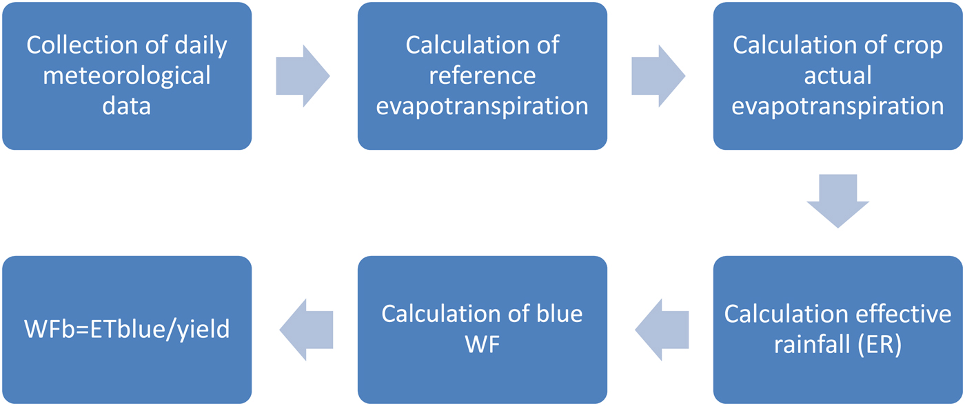
Fig. 2. Flowchart of blue water footprint (WFb).
Collection of daily meteorological data
Daily meteorological data of air temperature (minimum and maximum), relative humidity (minimum and maximum), solar radiation, wind and rainfall were collected for the year 2012 from 15 weather stations, managed by the agrometeorological service of Campania Region.
Calculation of reference evapotranspiration
The data set was used to calculate the reference evapotranspiration using the FAO model ET0 calculator (Allen et al., Reference Allen, Pereira, Raes and Smith1998; Raes, Reference Raes2009), which estimates ET0 from meteorological data by means of the FAO Penman–Monteith equation (Allen et al., Reference Allen, Pereira, Raes and Smith1998). The software used for this calculation works with dynamic daily climatic data.
Calculation of crop actual evapotranspiration
Daily crop evapotranspiration was calculated for the growing period (from sowing to harvest) of each crop by multiplying ET0 by the corresponding crop coefficient (K c). Specific dynamic values for Southern Italy of K c were collected for the initial, development, mature and final stages of each crop. Finally, for each crop, the total crop evapotranspiration (E tc) was calculated as the summation of daily crop evapotranspiration during the growing period.
Calculation of effective rainfall
Effective rainfall is the only part of total rainfall that is really usable by plants, excluding what is lost by surface runoff, deep percolation and interception by the canopy, and is a more realistic estimation of the moisture available to the soil. The method of the Soil Conservation Service of the United States Department of Agriculture (USDA SCS, 1994) was applied to estimate ER. This method estimates ER by processing long-term climatic and soil moisture data (50 years) recorded by 22 experimental stations representing different climatic and soil conditions.
Calculation of blue water footprint
The blue water evapotranspiration (ETblue) has been estimated as the difference between the total ETc and the ER; when ER > ETc, ETblue is zero (Hoekstra et al., Reference Hoekstra, Chapagain, Aldaya and Mekonnen2011). In the calculation of ETc and ER, a factor of 10 was used to convert depth of water (mm) into volume (value m3/ha).
Consequently, WFb was estimated as the ratio between ETblue and crop yield (Eqn (1)):
 $$\hbox{WFb}{\rm \,= \, \hbox{E}}{\rm \hbox{T}}_{{\rm blue}}{\rm /}\hbox{yield}$$
The WFb was calculated on a monthly basis for each crop and for each province of Campania, from June to September, which coincides with the Italian irrigation season of the crops analysed.
Farm Accountancy Data Network data analysis
The FADN data and methodological approach allowed specific costs to be attributed to each production process and the use of production factors, such as water and labour, to be broken down and similarly attributed. This made possible the computation of these indicators at the farm level, by product. The FADN data were used to compute water applied (WA) via irrigation and to estimate irrigation water per kg of product, estimated as a ratio between WA and yield for each crop in the different provinces. The GM for a specific product is the difference between total revenues and the specific costs incurred in the production process, before taxes and depreciation of fixed structures.
The GM, being an aggregate of economic performance at the level of the production process but at the same time reflecting the entrepreneurial choices of the whole farm, can be used as an index for the economic evaluation of the individual production activities.
Once WFb was calculated, the GM per WFb and the WFb per job were defined.
Gross margin per blue water footprint
The GM per WFb (GMWFb, in m3/€) was calculated as the ratio of WFb (m3) and GM of a crop (€), defined as the gross financial result of the management of the farm for each crop (gross production−specific costs for each crop) (Eqn (2)). This indicator describes the potential economic efficiency of irrigation in terms of the WFb. High values of GMWFb, for a given quantity of WFb, determine a potentially higher economic productivity of water.
 $$\hbox{GMWFb}{\rm \, = \,} \hbox{GM}{\rm /}\hbox{WFb}\,(\hbox{m}^{\rm 3}\!{\rm /}€ {\rm )}$$
Blue water footprint per working hours
In order to consider the overall water productivity, in the current study the index ‘WFb per working hours (job WFb (JWFb))’ was proposed in order to measure the performance of irrigation in terms of working hours (i.e. number of working hours needed to produce 1 t of product for each crop).
The JWFb (m3/working hours) was determined as the ratio between the WFb (m3/ton) and J (working hours/ton of product) (Eqn (3)). From a social point of view, it shows how many jobs (and workers) are behind each unit of water used. This is especially important on a local scale, in countries and regions where jobs are scarce and agriculture is an important employment opportunity. In this context, lower values of the indicator indicate a greater value of the unit of water.
 $$\hbox{JWFb}{\rm \, =\, } \hbox{WFb}{\rm /}\hbox{J}\,(\hbox{m}^{\rm 3}{\rm /}\hbox{working}\,\hbox{hours)}$$
Statistical analysis
The average values of the variables extracted from the FADN were used and, in specific cases, the coefficient of variation (CV) was calculated.
The use of CV aimed at showing the extent of variability in relation to the average of the population (Eqn (4)). It is often expressed as a percentage, and is defined as the ratio of the standard deviation (σ) to the average (μ) (with μ ≠ 0):
 $$\hbox{CV} = \sigma /\mu $$
For the calculated indicators, WFb, GMWFb and JWFb, an analysis of variance was also performed.
Furthermore, the ‘analysis of efficiency’ of average quantity of WA for irrigation in terms of water, the working hours per hectare and the GM for the different crops was carried out.
Lastly, factors (structural and economic) affecting the performance of farms in terms of WFb were identified and measured. For this assessment, a multivariate ordinary least squares (OLS) regression model, a statistical method of analysis that estimates the relationship between one or more independent variables (Y) and multiple dependent variables (X), was implemented.
More specifically, the ‘WA per kilogram of product’ for each crop (WATAPP_LKG) was taken as the dependent variable, while education level, age and gender of the holder, type of farming, crops cultivated, farm size and area devoted to each crop, average yield per hectare, water supplied by irrigation per hectare, economic size of farms, number of workers per hectare and total cost, GM per hectare and per yield, geographical location (provinces), and the constant C (i.e. the intercept) were taken as independent variables.
The OLS was carried out at different levels. At first, it was carried out at regional level by considering all crops; then it was verified that the variables identified with the first regression were still significant when analysing the crops individually, always at the regional level. Finally, the analysis was repeated by taking a single crop (alfalfa) and one province (Caserta).
Results and discussion
Water efficiency
The study area is characterized by a typical Mediterranean climate, and the evaporative power of the atmosphere determined by the climatic conditions does not differ significantly in the different provinces (Fig. 3).

Fig. 3. Reference evapotranspiration (ET0) for each province of Campania during the year 2012.
The results demonstrated that the quantity of water distributed with irrigation is, in general, much higher compared with the volumes effectively required by the crops, even when to such requirements an additional volume of water is considered to compensate the irrigation efficiency (Table 4).
Table 4. Ratio between water applied and blue water for different crops in each province of Campania (q/ha)

Nevertheless, there was a wide variation among provinces in the quantities of water distributed for the same crop. In fact, lower values were registered for tobacco, maize and alfalfa, while potato had higher values.
In terms of WA and yield, large differences were observed between the different crops. In particular, the crop with the highest value of WA was potato (1.916 m3/ha), followed by tomato (1.711 m3/ha), while the crops with the highest yield were maize silage (51.6 t/ha) and tomato (Fig. 4).

Fig. 4. Comparison between water volumes applied (m3/ha) and yield (t/ha) for different crops in Campania.
Despite the differences in terms of TOF, yields and geographical location, the reasons for these differences can be attributed to several causes. An early indication is certainly to be found between the different irrigation systems used, as well as the different sources of water used by farmers; however, the available data did not allow such analysis.
Gross margin per blue water footprint
The economic value of water is a partial factor of productivity that measures how the system converts water into economic value. It can be presented in several different formats. In the current paper the GM, obtained by deducting intermediate consumption (costs for each agricultural product) from final agricultural production (value of crop output), was used.
The economic productivity, measured by GM, varied widely (Fig. 5). In particular, a clear difference between the crops cultivated for animal feeding and the other crops considered was noticed. Indeed, alfalfa and silage maize had the lowest value of GM.
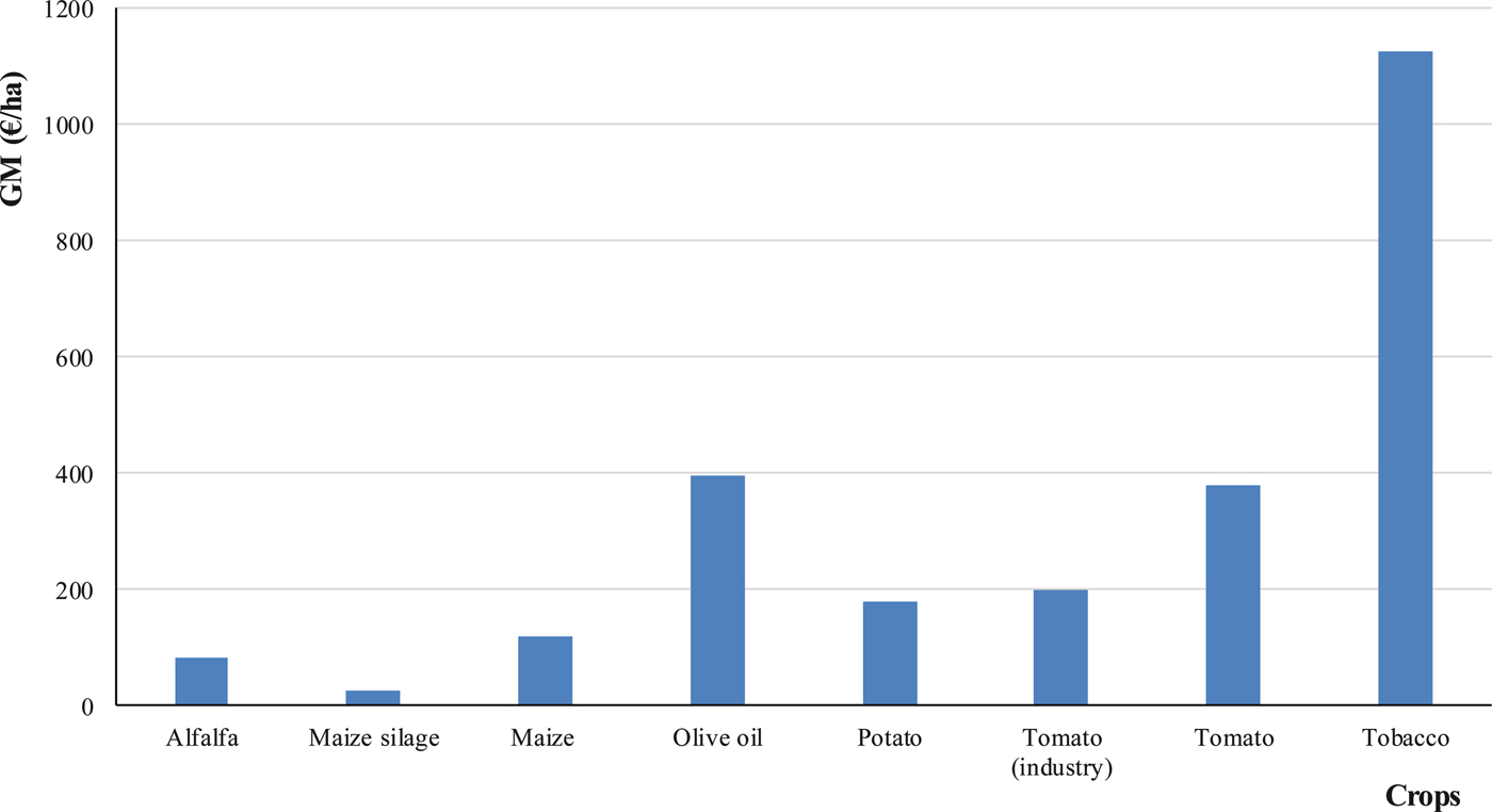
Fig. 5. Gross margin per hectare (€/ha) for different crops in Campania.
The comparison between water distributed with irrigation and the GM for the different crops in various provinces (Table 5) showed that the highest values were recorded for tobacco (1.38 m3/€) in Benevento, followed by tomato (1.12 m3/€) in Avellino. Looking at GMWFb of crops at a regional level, it can be first noticed that it was very variable among provinces (Fig. 6). In particular, silage maize had the highest value (23.89 m3/€) in Benevento, followed by maize in the same province (14.09 m3/€), while in Salerno a value of 6.78 m3/€ for alfalfa was estimated. Finally, olive, potato and tomato had the lowest GMWFb.
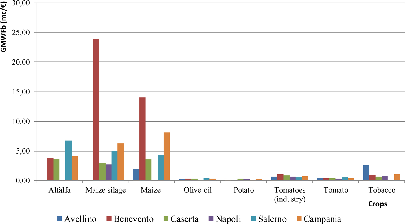
Fig. 6. Gross margin per blue water footprint (GMWFb; m3/€) for different crops in each province of Campania (June–Sept).
Table 5. Ratio between gross margin per hectare and average water applied for different crops in each province of Campania (€/m3)

The reasons for the observed differences should be found on one hand, in the amount of WA compared with the yield at provincial level and, on the other hand, in the difference in terms of GM observed. In particular, some crops had higher performance in terms of water (economic) productivity; in fact, in some cases higher yields were obtained with lower volumes of water.
Blue water footprint per working hour
The agricultural water productivity was also calculated in terms of employment in order to show how much labour is associated with the use of irrigation water for different crops. At the regional level, silage maize had the highest water use (m3) per working hour (154.08 m3/working hour), followed by alfalfa (148.58 m3/working hour) and maize (61.23 m3/working hour). The lowest values were those of potato (6.53 m3/working hour), tomato (5.58 m3/working hour) and olive (2.71 m3/working hour) (Fig. 7).
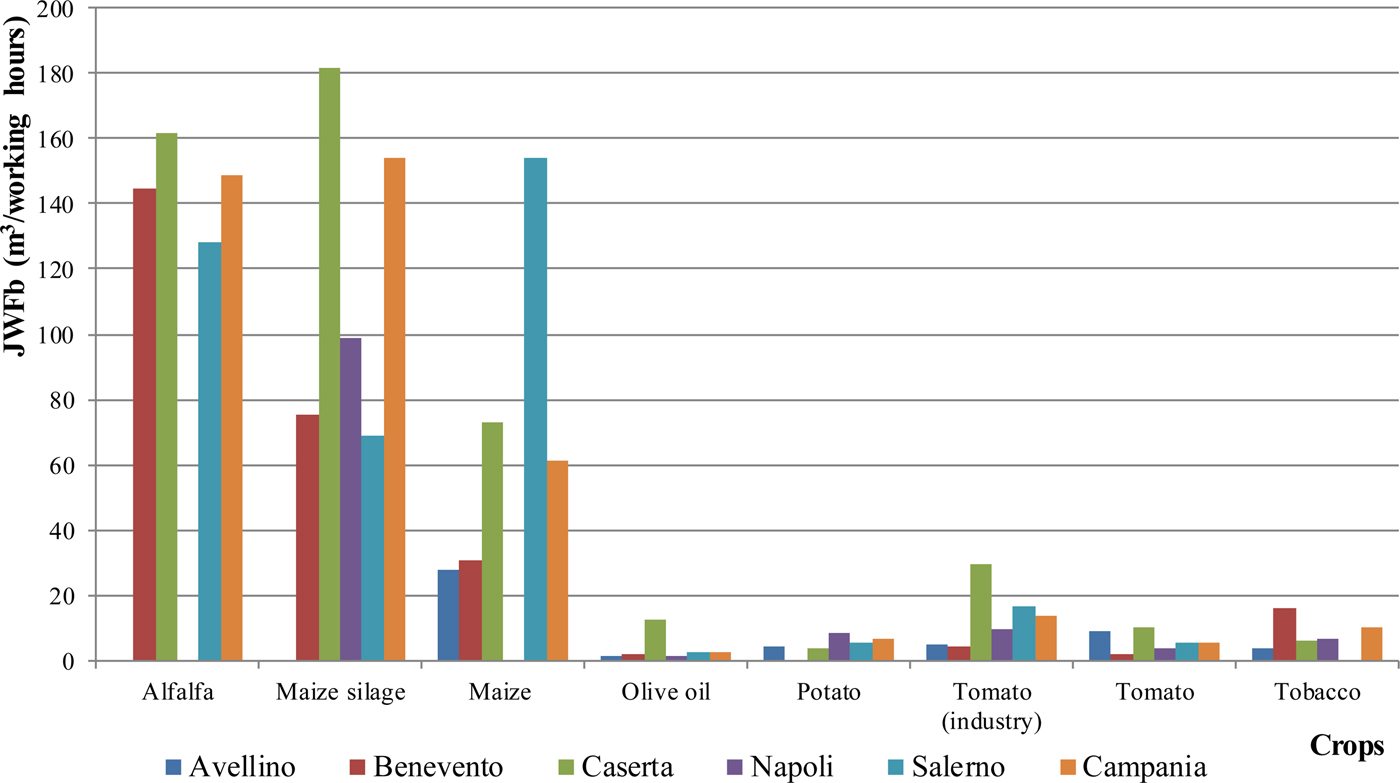
Fig. 7. Blue water footprint per working hour (JWFb; m3/working hours) for different crops in each province of Campania (June–Sept).
At the provincial level, the crop with the highest values of JWFb were always maize, alfalfa and silage maize. In particular, silage maize was the crop with the highest value of the index (181.68 m3/working hour) in Caserta, followed by alfalfa (161.68 m3/working hour) in Caserta and maize (154.28 m3/working hour) in Salerno. Conversely, lower values were found for olive – in particular, 1.75 m3/working hour in Benevento, 1.49 m3/working hour in Naples and, finally, 1.26 m3/working hour in Avellino. Among the other crops, lower values were those of potato with 3.53 m3/working hour in Caserta and 4.11 m3/working hour in Avellino, and tobacco with 3.94 m3/working hour in Avellino.
Tomato was the crop requiring the highest number of working hours per hectare of cultivation. In particular, in Benevento, it required 2318 h/ha and in Naples 1650 h/ha, followed by tomato for industry in Benevento (1000 h/ha), while alfalfa in Caserta is the crop requiring the lowest amount of work (28 h/ha). In general, the highest values were recorded for herbaceous crops (potato, tomato, tobacco); however, for the same crop, a strong variation among provinces was observed. Comparing the number of hours of work per hectare with the average WA for different crops in each province, it appears that Avellino recorded the highest value in the tomato industry (1.38 h/m3), tomato for consumer (1.25 h/m3) and tobacco (1.22 h/m3) (Table 6).
Table 6. Ratio between working hours per hectare and average water applied for different crop in each province of Campania (hours/m3)

The joint analysis of the two indices showed a clear difference between the crops linked to animal husbandry (alfalfa, maize) and the other crops taken into consideration (Figs 8 and 9). In fact, for the former, both the GMWFb and the JWFb achieved their highest values.
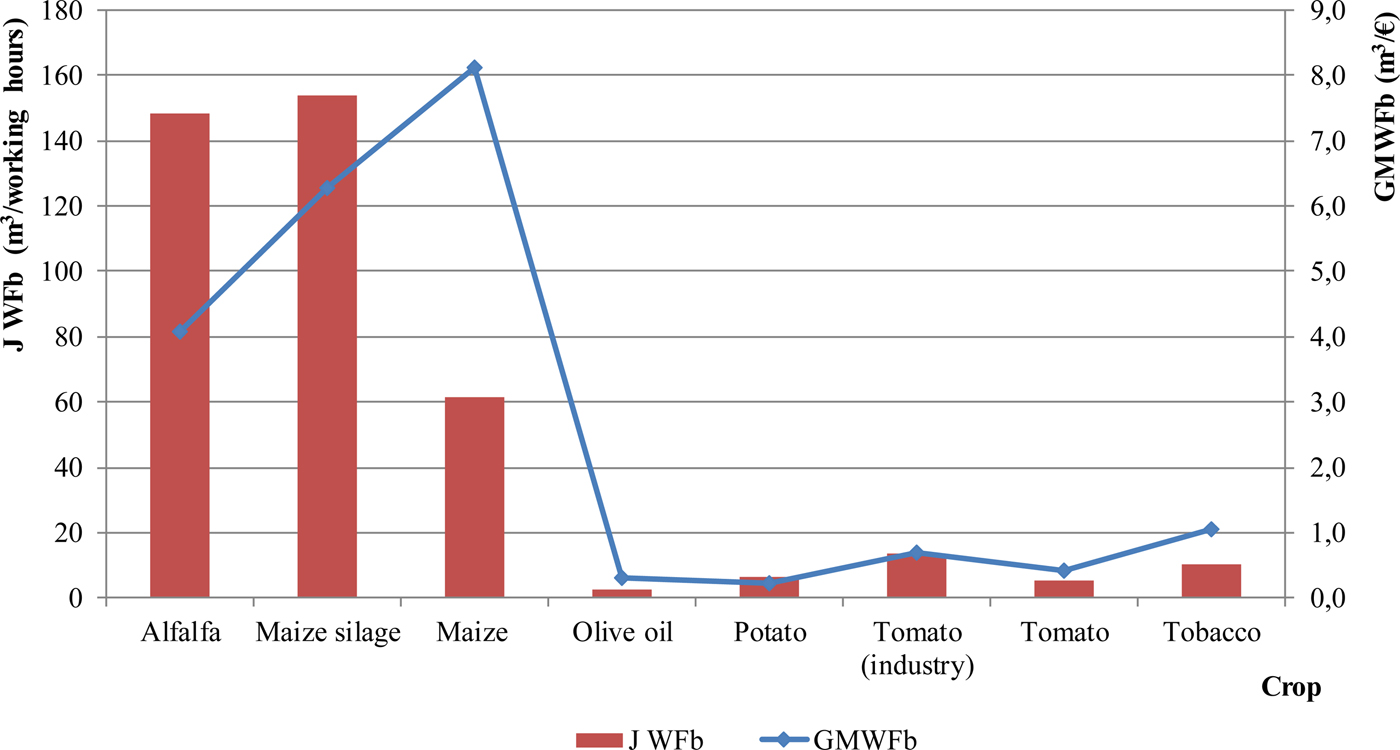
Fig. 8. Comparison between gross margin per blue water footprint (GMWFb; m3/€) and blue water footprint per working hours (JWFb; m3/working hours) for different crops in Campania.

Fig. 9. Comparison between gross margin per blue water footprint (GMWFb; m3/€), blue water footprint per working hour (JWFb; m3/working hours) and blue water footprint (WFb; m3/ton) for different crops in Campania.
Regarding the OLS results, the independent variables implemented in the model approximated the variables that have an effect on the performance of the farms in terms of WFb.
All the signs of the estimated coefficients are highly significant and consistent with expected signs. In particular, in the OLS, the statistically significant (P < 0.05) variables were geographical location (PROV), type of farming (TOF), crop (CROPS), yield (YIELD_Q_HA), WA (AV_WATER_APP), number of workers per hectare (NUM_MAN_HA), total cost per employee (TOT_COST_MAN) and, finally, GM for yield (GM_YIELD) and per hectare (GM_HA), in addition to the constant C.
Although some of the variables considered were not significant, some hypotheses can be formulated. In particular, the WA per kilogram of product seemed to be independent of the average farm size, economic size, age, sex and level of education of farmers and the area used for different crops. These results showed that there is ‘a way to irrigate’ which is common among farmers for each crop and per each study area that can be probably defined as ‘local knowledge’.
In the further OLS, only three crops were analysed – tomato (industry), maize and alfalfa – for which the independent variables that are significant (P < 0.05) varied according to crop. In the case of the tomato (industry), the only statistically significant variables were type of farming, yield per hectare, average volume of water distributed and GM per hectare; the results of maize showed that these are dependent on the total cost per worker and the yield per hectare. Finally, in the case of alfalfa, the statistically significant variables were GM per hectare and per yield as well as average volume of water distributed (Tables 7–11).
Table 7. Results of the one-way analysis of variance (ANOVA) for the indicators: blue water footprint (WFb), gross margin per blue water footprint (GMWFb), blue water footprint per working hour (JWFb)

Table 8. Ordinary least squares (OLS) regression model at regional level

C, constant; prov, provinces (geographical location); crops, crops cultivated; NUM_MAN_HA, number of workers per hectare; TOT_COST_MAN, total cost per employee; GM_YIELD, gross margin for yield; YIELD_Q_HA, yield; AV_WATER_APP, average water applied; GM_HA, gross margin per hectare.
Table 9. Results of the ordinary least squares (OLS) regression model at regional level for Tomato (industry)

C, constant; TOF, type of farming; YIELD_Q_HA, yield; AV_WATER_APP, average water applied; GM_HA, gross margin per hectare.
Table 10. Ordinary least squares (OLS) regression model at regional level for maize

C, constant; TOT_COST_MAN, total cost per employee; YIELD_Q_HA, yield.
Table 11. Ordinary least squares (OLS) regression model at region level for Alfalfa

GM_YIELD, gross margin for yield; AV_WATER_APP, average water applied; GM_HA, gross margin per hectare.
Results varied for the same crop at the provincial level (one crop in one province) (Table 12). In particular, for alfalfa cultivated in Caserta, the significant variables were total cost per worker, average volume of water distributed and GM per hectare and per yield.
Table 12. Results of the ordinary least squares (OLS) regression model for Alfalfa in the province of Caserta

TOT_COST_MAN, total cost per employee; GM_YIELD, gross margin for yield; AV_WATER_APP, average water applied; GM_HA, gross margin per hectare.
Finally, it was not possible to repeat the same analysis at the provincial level because, by dividing the number of farms between different provinces, there was no longer an adequate number of observations.
Conclusions
In the current study, some environmental, economic and social aspects related to the use of water for irrigation were investigated through the calculation of WFb-related indicators. In particular, WFb, GMWFb and JWFb were calculated for the main crops cultivated in the Campania region (South of Italy). The WFb, the volume of water used for the obtained yield, gives an indication of the impact of irrigation on the water resource. The GMWFb describes the economic productivity of irrigated agriculture in terms of the economic return of the blue water used. The JWFb expresses the social value of blue water in terms of job opportunities in (irrigated) agriculture.
Although irrigated agriculture can have significant impacts in terms of water consumption, it is also true that it has greater economic productivity (allowing a higher and more constant yield and allowing greater diversification of production). In the current research, for example, tomato, despite having the highest irrigation needs, had the highest GM and the largest number of working hours necessary for its cultivation. In other cases, such as alfalfa, a smaller volume of irrigation determined a substantial reduction of both the GM and the hours worked. Therefore, these indices confirmed that for certain irrigation volumes and for certain crops, the economic and social impacts are very different and the choice of an irrigated crop rather than another has different repercussions in terms of environmental and socio-economic sustainability.
Such a range of indicators would enable water managers and farmers to assess and compare production systems in terms of the different benefits that their use of water can provide: products, economic value, jobs. This can facilitate and support decisions at farm level, and investments and allocation of water at water basin level.
Considering the increasing impacts of climate change and variability on rainfall patterns, future research should also address the green component of the crop WF and assess the role of soil and crop management techniques to increase the water use efficiency in rain-fed agriculture.
Acknowledgements
The research work described in the present paper was undertaken as a part of COST Action ES1106 ‘Assessment of European Agriculture Water Use and Trade Under Climate Change’ (EURO-AGRIWAT). The authors gratefully acknowledge the GIS assistance of Dr Luigi Fabrizio Tascone, CREA. The authors would also like to thank Mr Bruce Polichar for his invaluable help in reading the English-language manuscript.
Financial support
This research received no specific grant from any funding agency, commercial or not-for-profit sectors.
Conflict of interest
None.
Ethical standards
Not applicable.


