


1. Introduction
The expansion of offshore wind farms into deeper water requires floating concepts, as bottom-fixed monopile turbines become prohibitively expensive beyond about  $60~\text {m}$ water depth (IRENA 2019). Such deep-water floating installations benefit from a more consistent and abundant wind resource as well as greater availability of potential deployment sites. In a floating concept, the tower, which supports the turbine, sits on a floater. The floater can be fully or partially submerged and is moored to the seabed. In this work, a catenary moored floater system is investigated. To avoid direct excitation by waves, such systems are typically designed to have long natural periods, typically above 25–30 s for pitch, roll, heave and yaw. For surge and sway modes, the natural periods are usually even longer, due to the absence of hydrostatic stiffness and low restoring force provided by the mooring. Since the hydrodynamic damping is weak, the systems are highly resonant. It is well known that low-frequency resonant motions of soft-moored structures can be excited by second-order difference-frequency hydrodynamic loads.
Here, we show that, for the floater considered, Morison drag forcing can also give rise to considerable resonant pitch motions. We focus on pitch motions because these are typically the most critical for turbine performance due to their direct influence on the effective inflow speed to the rotor. Surge motion is also relevant in this respect, though its effect is generally weaker due to the motions being slower. Large floater pitch motion can couple with the blade pitch control system of the turbine (Larsen & Hanson Reference Larsen and Hanson2007). Furthermore, extreme tower inclination angles induce strong overturning moments in the tower base (see e.g. Madsen, Pegalajar-Jurado & Bredmose Reference Madsen, Pegalajar-Jurado and Bredmose2019). Understanding the amplified resonant oscillations is of interest not only for the operational performance of the turbine, but importantly also for design so as to avoid structural fatigue and to maintain mooring system integrity.
A number of research studies on nonlinear hydrodynamic loads for offshore floating wind turbines have been carried out in recent years. Goupee et al. (Reference Goupee, Koo, Kimball, Lambrakos and Dagher2014) performed model-scale experiments in a combined wave and wind facility for three floater types supporting a scaled 5 MW turbine. The spar and semi-submersible floaters exhibited notable resonant subharmonic surge and pitch motions in the sea states and wind conditions tested. For the semi-submersible floater, Coulling et al. (Reference Coulling, Goupee, Robertson and Jonkman2013) successfully replicated the experiments numerically, accounting for second-order wave loads (in addition to wave-frequency and aerodynamic loading and the flexible behaviour of the tower). When the turbine was not operating (parked rotor with feathered blades), the difference-frequency wave forcing was shown to govern the global motion responses. Comparison of the (parked) floater dynamics, in a severe sea state with and without winds, revealed the nonlinear wave forcing to be dominant and the wind effects to be minimal (even in strong winds).
In contrast, in tests when the turbine was operational, the measured and simulated dynamics revealed dominance of the aerodynamic excitation of the slow-drift surge and pitch motions. These low-frequency motions were found to be similar for wind-only and wind-and-wave tests, though it should be noted that the tested sea state was fairly mild (see Coulling et al. Reference Coulling, Goupee, Robertson and Jonkman2013). Similarly, Roald et al. (Reference Roald, Jonkman, Robertson and Chokani2013) proposed that inclusion of second-order difference-frequency wave forcing is not essential for conditions when the turbine is operating based on a numerical study with a spar floater. Simulations carried out by Bayati et al. (Reference Bayati, Jonkman, Robertson and Platt2014) suggest that the subharmonic responses are dependent on both wind and wave environmental conditions. Their study highlighted the importance of the second-order difference-frequency hydrodynamics in severe wave conditions, while the wind slow-drift loads were shown to be dominant in a milder sea state.
As outlined above, investigating higher-order hydrodynamic effects is of interest, due to their relevance for high-speed wind conditions (above cut-out speed, so turbine parked) or when the turbine is not operating for other reasons such as faults, as well as for severe wave conditions under which the nonlinear hydrodynamic forcing is expected to dominate over aerodynamic effects. For accurate calculation of resonant motions in the absence of wind, both the slow-drift hydrodynamic excitation and the hydrodynamic damping levels are crucial (see Pegalajar-Jurado & Bredmose Reference Pegalajar-Jurado and Bredmose2019). In laboratory tests, however, both of these could be affected, for example due to difficulty of generating and then absorbing low-frequency wave components in a wave basin/flume and due to issues with scaling of viscous effects. A number of numerical modelling studies have reported difficulties in accurately predicting subharmonic resonant load and/or motion responses of floating wind turbines. The large code comparison initiatives OC5 and OC6 (see Robertson et al. Reference Robertson2017, Reference Robertson2020), as well as works by Azcona, Bouchotrouch & Vittori (Reference Azcona, Bouchotrouch and Vittori2019) and Li & Bachynski (Reference Li and Bachynski2021) for example, reveal model underestimation of surge and pitch resonant responses, when compared to wave-basin experiments. It is hoped that the detailed examination of small-scale floater measurements presented in this paper, which allow identification of different excitation mechanisms affecting the resonant floater dynamics, could be useful in model validation.
The aim of this paper is to present a comprehensive analysis of the dynamic motion of a model-scale floating wind turbine. We utilise harmonic separation, made possible by phase-manipulated realisations in the tank. All the stochastic sea states were run with phase inversion – a novelty for floating-structure response tests. The harmonic separation reveals even-harmonic, as well as unexpected odd-harmonic, components of the resonant responses. To identify the dominant hydrodynamic effects, we apply signal conditioning techniques, where the bandpass-filtered even- and odd-harmonic response is correlated with constructed proxy signals for the forcing. Second-order quadratic potential flow effects and Morison drag loading are shown to be important. The paper is organised as follows. First, in § 2, the floater characteristics and the experiments are outlined. In § 3, the signal processing techniques applied to the measured data are explained, and the nonlinear responses identified. Furthermore, in § 4, we quantify other potential sources of the resonant motion excitation.
2. Basin experiments
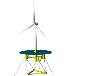
A comprehensive laboratory campaign investigating responses of a model-scale floating wind turbine under wave and wind forcing was carried out in 2017 in the deep-water basin at DHI, Hørsholm, Denmark. In this work, we focus on the hydrodynamics alone, analysing tests in the absence of wind. The tested turbine was a  $1:60$ scale model of the DTU 10 MW reference wind turbine. The TetraSpar floater (yellow structure in figure 1), designed by Stiesdal Offshore Technologies, consists of a main column connected to three sets of tanks, as well as a triangular counterweight suspended from these. Attached to the tanks, three catenary mooring chains (in a symmetric arrangement, with one line pointing down-wave, and two lines pointing obliquely up-wave) were used to soft-moor the floater. Here, we analyse the spar configuration where the tanks were completely submerged (leaving only the base of the tower column projecting through the free surface). A prototype of the TetraSpar floater design aims to reduce production and installation costs of floating offshore wind turbines by utilising simple tubular elements and by use of the counterweight. This counterweight can be lowered once the turbine has been towed to the deployment site, thus eliminating the need for deep-water harbours and/or the use of expensive offshore operations vessels (see Borg et al. (Reference Borg, Walkusch Jensen, Urquhart, Andersen, Thomsen and Stiesdal2020) for details of the full-scale deployment, with the floater installed in July 2021).

Figure 1. (a) Diagram of the wave basin, with wave gauges (blue) and the model (yellow). (b) Diagram of the model and (c) photograph of the experimental set-up. Note that in the spar configuration tested the buoyancy tanks are fully submerged. (d) Target (solid) and measured (dashed) free-surface variance density spectra  $S(\eta )$, together with the floating-system rigid-body natural frequencies
  $f_{ni}$ (details in tables 1 and 2). Note that the measured spectra are from a wave gauge located at
  $[x,y]=[5~\text {m},~10~\text {m}]$.
The wave basin is 30 m wide and 20 m long, with an absorbing beach and an articulated flap wavemaker hinged  $1.5~\text {m}$ above the basin floor (see figure 1). Linear wave generation was used for calculation of the paddle signals, and active absorption by the wavemaker was not utilised. The water depth was
  $3~\text {m}$, and we note that most of the beach structure at the far end of the basin was submerged. The model was positioned equidistantly from the basin sidewalls and
  $5~\text {m}$ away from the wavemaker (at
  $[x,y]=[5~\text {m},~15~\text {m}]$, where
  $x$ and
  $y$ denote the distance from and along the wavemaker). The relatively close placement of the model to the wavemakers was necessary for tests with wind forcing (not reported here) to ensure a consistent wind field over the swept rotor area produced by the wind generator. The influence of linear evanescent waves at the model location was examined to ensure that these local standing waves (originating from a velocity mismatch at the paddle face) did not contaminate the experiments. For all components in the incident wave frequency range, the summed evanescent wave amplitude at the model location was found to be less than 0.5 % of the corresponding progressive component. Hence, these standing waves almost completely decayed away, and their effect on the floater motions was negligible.
Free-surface elevations were measured with 10 wave gauges. Measurement from the wave gauge at  $[x,y]=[5~\text {m},~10~\text {m}]$, which is offset from the model laterally, is assumed to represent the undisturbed wave field (i.e. in the absence of the model) and is used in the conditioned signal analysis. This is deemed appropriate due to the slender geometry of the floater (with the diameter of the widest tubular element being
  $0.11~\text {m}$ in model scale). The scattered and the radiated wave fields are therefore relatively small, and their effect on gauge measurements at
  $[x,y]=[5~\text {m},~10~\text {m}]$ is further reduced due to the geometric spreading associated with radially propagating waves. The wave gauges placed along the basin centreline were utilised in the second-order error wave and basin sloshing investigations; in particular, readings from the wave gauge closest the wavemaker at
  $[x,y]=[1~\text {m},~15~\text {m}]$ are used in § 4.2. A Qualisys optical motion tracking system was employed to measure the six-degree-of-freedom motions of the floater. An extensive range of additional instrumentation was employed to measure tower and nacelle accelerations, mooring line and counterweight line loads, as well as rotor behaviour. Further details of the campaign are given in Borg et al. (Reference Borg, Bredmose, Stiesdal, Jensen, Mikkelsen, Mirzaei, Pegalajar-Jurado, Madsen, Nielsen and Lomholt2018). See also Bredmose et al. (Reference Bredmose2017) for details on the model turbine.
In the experimental campaign, long-duration irregular wave tests were performed and are examined here. We note that regular waves and focused wave group tests were also carried out. All conditions were long-crested, and in this work only waves propagating in the  $x$-direction are presented (i.e. propagation direction normal to the wavemaker front). The analysed sea states are listed in table 1; a Pierson–Moskowitz spectral shape was used for all conditions. Sea states EC5, EC6 and EC64 can be considered operational, whereas EC11 represents a survival extreme-conditions test. The long-duration runs were 3 h long (in full scale), roughly corresponding to between 600 and 1600 wave periods for the longest and shortest waves tested. We note that, apart from the longest-period sea state (with
  $k_p d = 2.3$, where
  $k_p$ is the wavenumber corresponding to peak period
  $T_p$ and
  $d$ is water depth), the conditions can be considered deep-water. In order to facilitate separation of individual harmonics under the broad-banded wave conditions, phase-manipulated tests were carried out. For each sea state, two realisations were performed: the first one with randomly chosen phases, the second one with the phase of every component shifted by
  $180^{\circ }$. We note that this is equivalent to inverting the linear paddle signal, which is very convenient from a practical point of view. Such pairs of tests are used in § 3.1, where harmonic separation is discussed.
Table 1. Environmental conditions used in the experimental campaign. Sea states are given in terms of significant wave height  $H_s$ and peak period
  $T_p$, with Pierson–Moskowitz spectral shape. Model-scale values are shown in parentheses.

The precise details of the model floater, tower and turbine will be omitted here for brevity. The natural frequencies of rigid-body motions of the system are detailed in table 2. The values were estimated from free-decay tests carried out as part of the campaign. The mismatch of the surge and sway natural periods is thought to originate from a slight deviation from symmetry in the experimental set-up. These experimentally derived natural periods were closely matched by calculations using the system mass properties and the linearised mooring and hydrostatic restoring forces.
Table 2. Natural periods of the tested system  $T_{ni}$, where
  $i=1, \ldots, 6$ denotes the floater rigid-body motion modes of surge, sway, heave, roll, pitch and yaw, respectively. Values of the natural frequencies
  $f_{ni} = {1}/{T_{ni}}$ are also given for convenience. Model-scale values are shown in parentheses.

3. Identifying nonlinear resonant responses
The measured floater surge, heave and pitch motions exhibit responses in the range of the incident wave energy, as well as in the subharmonic range peaking at the respective natural frequencies. Figure 2 shows short segments of the wave and pitch motion signals from two sea states. The notable low-frequency motions are clearly seen. In addition, pitch motion spectra for the four wave conditions investigated are displayed later in figure 4. Since, for the floater considered, the natural frequencies of all six degrees of freedom lie below the incident wave frequencies (see figure 1), the motion at the natural frequencies must be driven nonlinearly. The analysis that follows identifies the source of these resonant subharmonic motions.

Figure 2. Measured free surface  $\eta$ and floater pitch motion
  $\theta$ time series. (a,b) Total undisturbed free surface. (c,d) Total pitch. (e,f) High-pass-filtered (HPF) odd-harmonics signal representing linear wave-frequency pitch motion. (g,h) Even-harmonics signal (red) and low-pass-filtered (LPF) odd-harmonics signal (blue) both representing subharmonic pitch motion.
3.1. Harmonic separation
Utilising the two phase-shifted realisations (the original and the inverted test), odd and even harmonics can be separated via subtraction and addition of the two signals (e.g. Jonathan & Taylor Reference Jonathan and Taylor1997; Fitzgerald et al. Reference Fitzgerald, Taylor, Eatock Taylor, Grice and Zang2014):
 \begin{equation} \left. \begin{aligned} \text{odd} \quad & \frac{1}{2} (X_0 - X_{180}) \nonumber \\ & \quad = \mathrm{Re} \sum_{n} A_n Q^{(1)}_{n} \mathrm{e}^{\mathrm{i} 2 {\rm \pi}f_n t} + \cdots \nonumber \\ & \qquad + \mathrm{Re} \sum_{n} \sum_{m} \sum_{p} A_n A^{-:*}_m A^{-:*}_p Q^{(3\pm)}_{n,m,p} \, \mathrm{e}^{\mathrm{i} 2 {\rm \pi}(f_n \pm f_m \pm f_p) t} + O(A^{5}), \nonumber \\ \text{even} \quad & \frac{1}{2} (X_0 + X_{180}) \nonumber \\ & \quad = \mathrm{Re} \sum_{n} \sum_{m} A_n A^{-:*}_m Q^{(2\pm)}_{n,m} \mathrm{e}^{\mathrm{i} 2 {\rm \pi}(f_n \pm f_m) t} + O(A^{4}), \end{aligned} \right\} \end{equation}
where  $X_0$ and
  $X_{180}$ represent the two phase-shifted signals. In the above,
  $A_n= |A_n| \mathrm {e}^{\mathrm {i} \varphi _n}$ and
  $Q_n^{(1)}$ denote the complex wave amplitude and the complex linear transfer function of an
  $f_n$ frequency component, with
  $\varphi _n$ being the phase of the wave component. The superscript
  $^{-:*}$ denotes complex conjugation, which only applies to subharmonic components. The double and triple summations each comprise both super- and subharmonics, with coefficients
  $Q^{(2\pm )}_{n,m}$ and
  $Q^{(3\pm )}_{n,m,p}$ representing second- and third-order transfer functions/interaction kernels, respectively. Further details on higher harmonic components are provided in Appendix B. The reason the subtraction and addition time series contain the odd and even harmonics, respectively, becomes clear when one considers the individual complex amplitudes in the inverted signal, which are given by
  $|A_n| \mathrm {e}^{\mathrm {i} (\varphi _n + {\rm \pi})} = - A_n$. With the complex amplitudes pre-multiplied by a minus sign, all odd-harmonic terms become inverted while the even-harmonic terms remain unaffected in the inverted signal.
This phase-based harmonic separation method relies on a Stokes-like structure of the studied wave-driven response. It has been used to analyse various nonlinear wave phenomena involving fixed (Fitzgerald et al. Reference Fitzgerald, Taylor, Eatock Taylor, Grice and Zang2014; Zhao et al. Reference Zhao, Wolgamot, Taylor and Eatock Taylor2017; Chen et al. Reference Chen, Zang, Taylor, Sun, Morgan, Grice, Orszaghova and Tello Ruiz2018) and floating (Roux de Reilhac et al. Reference Roux de Reilhac, Bonnefoy, Rousset and Ferrant2011; Chen et al. Reference Chen, Taylor, Ning, Cong, Wolgamot, Draper and Cheng2021) offshore structures, as well as higher-order responses in coastal problems (Orszaghova et al. Reference Orszaghova, Taylor, Borthwick and Raby2014; Whittaker et al. Reference Whittaker, Fitzgerald, Raby, Taylor, Orszaghova and Borthwick2017; Judge et al. Reference Judge, Hunt-Raby, Orszaghova, Taylor and Borthwick2019). The above studies utilise short deterministic wave groups. More recently, the method has been applied to random time series (Adcock et al. Reference Adcock, Feng, Tang, van den Bremer, Day, Dai, Li, Lin, Xu and Taylor2019; Zheng et al. Reference Zheng, Lin, Li, Adcock, Li and van den Bremer2020; Kristoffersen et al. Reference Kristoffersen, Bredmose, Georgakis, Branger and Luneau2021), which we also pursue here.
To illustrate the frequency range of the various harmonics, figure 3 shows the free-surface variance density spectra for the free linear components and the associated second- and third-order bound waves. Details of the spectral calculations are included in Appendix B. For clarity, a broad-banded top-hat spectral shape with clearly defined cutoff frequencies  $f_{min}$ and
  $f_{max}$ is shown, in addition to sea state EC5. As seen from the spectral plots, the individual harmonics cannot be easily separated via frequency filtering due to them overlapping, highlighting the usefulness of the harmonic separation using phase-manipulated realisations. We note that straightforward frequency filtering is only possible for very narrow-banded processes.

Figure 3. Theoretical free-surface variance density spectra  $S(\eta )$: (a) Pierson–Moskowitz input spectrum EC5, with linear wavemaking up to 2.5 Hz; and (b) top-hat input spectrum with frequency range
  $(f_{{min}}, f_{{max}}) = (0.5,~2.5~\text {Hz})$ and
  $H_s = 0.069~\text {m}$ (same as EC5). Curves shown are: linear free wave spectrum
  $S^{(1)}$ (black); second-order difference-frequency bound wave spectrum
  $S^{(2-)}$ (red); second-order sum-frequency bound wave spectrum
  $S^{(2+)}$ (purple); third-order difference-frequency bound wave spectrum
  $S^{(3-)}$ (blue); and third-order sum-frequency bound wave spectrum
  $S^{(3+)}$ (green). Note that only the low- and high-frequency tails of the third-order difference-frequency spectrum
  $S^{(3-)}$ are shown. The solid green vertical line denotes the pitch natural frequency
  $f_{n5}$.
Within the even-harmonics signal, the second-order difference-frequency components (terms with  $Q_{n,m}^{(2-)}$ in (3.1) and denoted by
  $S^{(2-)}$ in figure 3) span frequencies within
  $(0,~f_{{max}} - f_{{min}})$, which includes the pitch natural frequency. The second-order sum-frequency components (terms with
  $Q_{n,m}^{(2+)}$ in (3.1) and denoted by
  $S^{(2+)}$ in figure 3) comprise frequencies
  $(2 f_{min}, 2 f_{max})$, so do not extend to the low-frequency subharmonic range where the natural frequencies lie. The second-order super- and subharmonics can be suitably separated by frequency filtering.
Now inspecting the odd-harmonics signal, the third-order superharmonic (terms with  $Q_{n,m,p}^{(3+)}$ in (3.1) and denoted by
  $S^{(3+)}$ in figure 3) is typically centred around
  $3 f_p$ in frequency and can be isolated by frequency filtering. However, the linear components (terms with
  $Q_n^{(1)}$ in (3.1) and denoted by
  $S^{(1)}$ in figure 3) and the third-order subharmonic components (terms with
  $Q_{n,m,p}^{(3-)}$ in (3.1) and denoted by
  $S^{(3-)}$ in figure 3) cannot be separated, as their frequency ranges overlap. As detailed in Appendix B, the third-order subharmonic terms arise from
  $++-$,
  $+-+$ and
  $+--$ combinations of linear frequencies. Their frequency range is
  $(\max (0,~2f_{min} - f_{max}),~2f_{max} - f_{min})$, and as such they extend below and above the linear frequency range. Due to singularities in the third-order subharmonic transfer function
  $Q_{n,m,p}^{(3-)}$, only the low- and high-frequency tails of the spectrum
  $S^{(3-)}$ are shown in figure 3. We note that the low-frequency range spans the pitch natural frequency.
The harmonic separation is applied to both the free surface  $\eta$ and the pitch motion
  $\theta$ experimental signals. Careful alignment of the measured signals
  $X_0$ and
  $X_{180}$ is critical in ensuring correct cancellation of the relevant harmonics and in avoiding spectral leakage. The linearised free surface
  $\eta _L$ is obtained from the odd-harmonics free-surface signal, which has been low-pass-filtered to remove third- and higher-order odd superharmonic content. In the remaining signal, the third-order subharmonic bound wave content is very small, due to the (mostly) deep-water conditions analysed here. For this reason, the low-pass-filtered free-surface subtraction time series is taken to represent linear waves.
Figure 4 shows spectra of the total (dotted black), as well as the even (solid red) and the odd (solid blue) pitch motion. We would expect the response at the low natural frequency to appear in the even signal due to second-order subharmonic wave–floater interactions. However, for the longer sea states EC11 and EC64, a comparably large response at the pitch natural frequency also manifests in the odd signal. As mentioned above, there is virtually no linear excitation at the natural frequency. The fact that this motion is not driven linearly is confirmed by calculation of linear motion (dashed blue), which completely fails to reproduce the response peak at the natural frequency. This calculation uses a theoretical linear transfer function for pitch motion (based on the work of Pegalajar-Jurado, Borg & Bredmose (Reference Pegalajar-Jurado, Borg and Bredmose2018)) applied to the linearised free surface  $\eta _L$. Further details can be found in Appendix A. The linearised hydrodynamic damping estimates are taken from Pegalajar-Jurado, Madsen & Bredmose (Reference Pegalajar-Jurado, Madsen and Bredmose2019). Their analysis of this experimental campaign reveals the pitch damping to be dependent on sea state severity, with the damping values positively correlated with the significant wave height
  $H_s$.

Figure 4. Measured floater pitch motion variance density spectra  $S(\theta )$: total, odd and even components, respectively, are shown in dotted black, solid blue and solid red lines. The dash-dotted blue curve represents the reconstructed linear pitch motion via application of the linear transfer function to the linearised free surface. The solid green and the dashed black vertical lines denote the pitch natural frequency
  $f_{n5}$ and the input peak wave frequency
  $f_p$, respectively.
For all conditions tested, the odd-harmonics pitch motion spectra exhibit a clear frequency gap between the resonant and the wave-frequency responses (see figure 4). Frequency filtering can thus be carried out with the cutoff frequency chosen to correspond to the spectral minimum in the gap. The separated pitch motion time series are shown in figure 2. The high-pass-filtered (HPF) odd-harmonics signal represents linearly excited pitch motions. The resonant subharmonic pitch motions comprise contributions from the even-harmonics signal and the low-pass-filtered (LPF) odd-harmonics signal.

Figure 5. Theoretical variance density spectra  $S$. Linear free wave spectrum for sea state EC5 denoted by
  $S^{(1)}$ (black). Difference- and sum-frequency spectral content of
  $\eta _L^{2}$ denoted by
  $S^{-}(\eta _L^{2})$ (red) and
  $S^{+}(\eta _L^{2})$ (purple), respectively. Difference- and sum-frequency spectral content of
  $\eta _L^{3}$ denoted by
  $S^{-}(\eta _L^{3})$ (blue) and
  $S^{+}(\eta _L^{3})$ (green), respectively. Spectrum of
  $u_L|u_L|$ denoted by
  $S(u_L|u_L|)$ (light blue). Note that the curves are scaled and as such the vertical axis range is omitted. The solid green vertical line denotes the pitch natural frequency
  $f_{n5}$.
3.2. Fluid forcing proxies
The nonlinear resonant pitch motions comprise both even and odd harmonics. The odd response is somewhat unexpected, as one would typically assume the subharmonic resonant motions to arise from second-order potential flow wave–structure interactions. The spectral content of the second- and third-order bound waves is seen to encompass the pitch natural frequency, suggesting quadratic and cubic interactions as plausible loading mechanisms. Additionally, we also consider Morison drag loading, as its frequency content is also relevant in the subharmonic range. In our data-driven analysis approach, we utilise proxies for the three possible forcings at play.
The linearised free surface raised to the  $n{\text {th}}$ power, i.e.
  $\eta _L^{n}$, represents the
  $n{\text {th}}$-order bound waves (and in fact other wave properties/contributions), assuming unit transfer function values. It is thus a proxy for the
  $n{\text {th}}$-order potential flow forcing, which is generally due to contributions from both the local
  $n{\text {th}}$-order processes and scattering of the
  $n{\text {th}}$ harmonic of the incident wave. Figure 5 shows spectra of the sum- and difference-frequency content of the
  $\eta _L^{2}$ and
  $\eta _L^{3}$ signals, where here
  $\eta _L$ denotes a linear synthetic, rather than the linearised experimental, free-surface signal. The difference-frequency content of the squared and cubed signals is given by
  $( \eta _L^{2} + [\text {H}(\eta _L)]^{2} )/2$ and
  $3\eta _L (\eta _L^{2} + [\text {H}(\eta _L)]^{2})/4$, respectively, where
  $\text {H}$ denotes the Hilbert transform, which introduces a
  $90^{\circ }$ phase shift into the signal. The equivalent expressions for the sum frequencies are
  $( \eta _L^{2} - [\text {H}(\eta _L)]^{2} )/2$ and
  $\eta _L ( \eta _L^{2} -3 [\text {H}(\eta _L)]^{2} )/4$, and follow from Walker, Taylor & Eatock Taylor (Reference Walker, Taylor and Eatock Taylor2004). The magnitudes of these proxy forcing signals are irrelevant and as such the spectra presented in figure 5 have been scaled to aid comparison with figure 3. As expected, the proxy signals have comparable spectral content to the bound wave components.
In addition to potential flow forcing, we consider viscous effects and approximate these via the drag term of the Morison equation (see Morison, Johnson & Schaaf Reference Morison, Johnson and Schaaf1950). Following the approach of Pegalajar-Jurado & Bredmose (Reference Pegalajar-Jurado and Bredmose2019), we can expand the relative velocity formulation of the drag term (see e.g. Faltinsen Reference Faltinsen1993) into a pure forcing term that is independent of the body velocity, as well as linear and quadratic damping terms. We choose the drag forcing proxy to be  $u_L|u_L|$, where
  $u_L$ represents the linearised experimental horizontal fluid velocity at the mean free surface and
  $|{~}|$ represents the modulus. Assuming deep water, we evaluate the velocity signal using the linearised free-surface measurement
  $\eta _L$ such that
  $u_L = \text {H}[\dot {\eta }_L]$, where the dot operator
  $\dot {~}$ denotes time differentiation. The frequency content of the drag forcing proxy is shown in figure 5. The spectrum can be seen to have a peak around
  $f_p$ and
  $(3\text {--}4)f_p$, similar to the third-order potential flow terms. The low-frequency components extend below the linear range and span the natural frequencies, thus possibly exciting the resonant motions.
To our knowledge, a closed-form expression for the  $u_L|u_L|$ signal using a broad-band harmonic content of
  $u_L$, similar to the summation expressions given in (3.1) for the second- and third-order potential flow terms, is not possible. We can only write a regular wave approximation, with simple sinusoidal velocity
  $u_L=a\cos (\omega t + p)$, which reads
 \begin{align} & a\cos(\omega t + p)\, |a\cos(\omega t + p)| \nonumber\\ & \quad = \frac{8}{3 {\rm \pi}} a^{2} \cos(\omega t +p) + \frac{8}{15 {\rm \pi}} a^{2} \cos(3\omega t +3p) \nonumber\\ & \qquad +\sum_{n=2}^{\infty} \frac{({-}1)^{(n+1)} 8 a^{2} } {(2n-1)(2n+1)(2n+3){\rm \pi}} \cos((2n+1)\omega t + (2n+1) p) . \end{align}
The above is an infinite summation of progressively smaller odd-harmonic terms, with no even harmonics. The drag forcing signal is thus dominated by the components close to the linear spectral peak, as can be seen in figure 5. It is worth presenting here the third-order potential flow forcing proxy for a sinusoidal linear signal, which is given by
 \begin{equation} ( a\cos(\omega t + p) )^{3} = \tfrac{3}{4} a^{3} \cos(\omega t +p) + \tfrac{1}{4} a^{3} \cos(3\omega t + 3 p). \end{equation}
The first term represents the subharmonics, the second term the superharmonics.
Comparing (3.2) and (3.3), we note a number of similarities and differences. In a Stokes-like harmonic structure, an  $n{\text {th}}$ harmonic can be approximated to be proportional to
  $a^{n} \cos (n \omega t + n p)$, i.e. it scales as the
  $n{\text {th}}$ power of the linear amplitude. We note that the complete expression also contains higher-order subharmonic terms, which scale as the
  $(n+2m){\text {th}}$ power of the linear amplitude, and as such are much smaller. The third-order effects investigated here are precisely such higher-order subharmonic terms of the first harmonic (see the first term in (3.3), terms with
  $Q_{n,m,p}^{(3-)}$ in (3.1) and denoted by
  $S^{(3-)}$ in figure 3). The key point is that Stokes odd harmonics only have odd amplitude power scalings. On the other hand, in the drag forcing expression, all harmonics depend quadratically on the linear amplitude, so the amplitude scaling is independent of the harmonic number. The relationship between the harmonic number and the amplitude power is thus different. Focusing on the first harmonic
  $\omega$ components in the two expressions, as these are most relevant for the analysis here, we note their phase alignment. Extrapolating to a broad-banded situation, we anticipate the two forcing signals to be strongly correlated, and to scale respectively as a square and a cube of the linear content amplitude.
As we are interested in the resonant pitch motion, we bandpass filter (BPF) all the response and the forcing proxy signals around the natural frequency (roughly between  $0.75 f_{n5}$ and
  $1.20 f_{n5}$). We note that the strong similarity in shape between the BPF drag and the BPF third-order loading signals remains. This is illustrated in figure 6 for sea state EC11, where the experimental linearised free surface
  $\eta _L$ was used. The assumed amplitude scaling between the BPF
  $u_L|u_L|$ and the BPF
  $\eta _L^{3}$, i.e. power coefficient of
  ${3}/{2}$, will be utilised in analysis presented in § 3.4.

Figure 6. Third-order potential flow forcing  $\eta _L^{3}$ and Morison drag forcing
  $u_L|u_L|$ proxy signals for sea state EC11 calculated using the experimental linearised free-surface signal
  $\eta _L$: (a) raw signals and (b) bandpass-filtered (BPF) signals.
3.3. Conditioned signal analysis
In order to identify the source of the pitch motion at the natural frequency, we use signal conditioning (similar to Zhao et al. (Reference Zhao, Taylor, Wolgamot and Eatock Taylor2018)). The conditioning analysis involves selecting a number (here 30) of the largest events in the conditioning signal, as well as the corresponding sections of the conditioned signal. A portion of time series around each identified peak is cut out, followed by shifting of each time axis such that the maximum value occurs at zero relative time, and finally the 30 series are averaged. The remaining structure in time of the averaged signals is indicative of the coupling between the two processes. This is because the averaged conditioned signal would simply reduce to zero-mean noise if there was no phase relationship to the conditioning process.
Figures 7 and 8 show the even and odd pitch motion conditioned on second and third powers of  $\eta _L$ as well as on
  $u_L|u_L|$, with all signals having been suitably bandpass-filtered. The conditioning signals are locally symmetric, as expected. For all sea states, the plots clearly show a coupling between
  $\eta _L^{2}$ and even-harmonic pitch (left-hand-side panel for each sea state, i.e. panels (a) and (d) in Figures 7 and 8), confirming that these motions are caused by quadratic interactions. For sea states EC6 and EC11, strong coupling is also strikingly demonstrated between the odd-harmonic pitch signals and both the
  $\eta _L^{3}$ and
  $u_L|u_L|$ forcing proxies (middle and right-hand-side panels respectively, i.e. panels (e) and (f) respectively for sea state EC6 in Figure 7 and panels (b) and (c) respectively for sea state EC11 in Figure 8). The fact that the pitch motions correlate with both conditioning signals is consistent with figure 6, which shows their shape similarity. For the shortest and longest sea states EC5 and EC64, however, these couplings appear less well defined, as the expected response is mostly hidden within the noise band.

Figure 7. Conditioned signal analysis for sea states EC5 (a–c) and EC6 (d–f). Local average profiles of bandpass-filtered (BPF) even-harmonics and odd-harmonics pitch motion (second and third rows, respectively, in each panel, for each sea state) conditioned on extrema in the BPF  $\eta _L^{2}$,
  $\eta _L^{3}$ and
  $u_L|u_L|$ time series (first row in each panel, for each sea state). The grey shading represents
  $95\,\%$ confidence intervals on the estimation of the mean signals. Reciprocity is shown by the dash-dotted curves, which correspond to the scaled and time-reversed conditioned forcing signals. In the label, the symbol
  $|$ represents ‘conditioned on’.

Figure 8. As in figure 7, but for sea states EC11 (a–c) and EC64 (d–f).
The conditioned signal analysis can also be performed in reverse, whereby we condition on large even/odd pitch events. The equivalent plots to figures 7 and 8 are omitted for brevity. However, we utilise the resulting conditioned signals to highlight reciprocity between the two sets of coupled processes. For a linear system of two Gaussian processes (with a linear relationship between input and output), the averaged output signal conditioned on an extreme input event is identical to the scaled time-reversed/mirrored averaged input signal conditioned on an extreme output event. The derivation of this reciprocity relation is omitted here, but can be found in Zhao et al. (Reference Zhao, Taylor, Wolgamot and Eatock Taylor2018), for example. The additional dash-dotted curves in figures 7 and 8 show the mean forcing time histories that give the largest pitch response. Note that the time axis has been reversed for the  $\eta _L^{n}$ and
  $u_L|u_L|$ forcing time series and that the curves have been scaled.
For the even pitch and the assumed  $\eta ^{2}$ loading, each pair of these reciprocity curves, where above the noise levels, shows a distinct similarity. We note, of course, that the second-order potential flow quadratic interactions are pairwise in frequency. However, between a higher-order response and the corresponding higher-order forcing signal there is a linear relationship. In other words, the nonlinear forcing operates on a linear hydromechanical system through a linear transfer function, which we have confirmed with this reciprocity analysis. It follows from Stokes theory that the second-order subharmonic bound wave content in the undisturbed incident waves is very low for the (mostly) deep-water conditions analysed in this work. Moreover, as the structure considered is rather slender, the identified nonlinear responses are presumably excited by local quadratic processes at the structure, as opposed to the incident or diffracted bound wave components. This agrees with Simos et al. (Reference Simos, Ruggeri, Watai, Souto-Iglesias and Lopez-Pavon2018), who carried out a comprehensive numerical investigation of second-order difference-frequency wave forcing of a semi-submersible floating turbine. Their study demonstrated that in deep water the second-order diffraction contribution is negligible, and thus the second-order forcing follows primarily from the quadratic/product terms of first-order wave and body variables.
The reciprocity analysis for the odd pitch motions appears to work equally well for the third-order and the drag loading proxies. Clearly there cannot be a linear relationship between the odd resonant motions and both the forcings. We postulate that, due to averaging over only a limited number of events (spanning a range of amplitudes), we are unable to determine which of the two processes is driving the odd pitch motions. We note that, since the conditioned time histories are so similar (in magnitude and shape), it could be that both effects are present and provide roughly equal excitation. Additional processing of the data presented in the next section will reveal the dominant effect.
Lastly, we briefly comment on the surge and heave motions of the TetraSpar floater. Analysis equivalent to that presented in figure 4 suggests that, in these modes, the subharmonic odd responses are not as significant, and that the resonant motions are driven by second-order interactions. We also note that bi-spectral (and tri-spectral) analysis (see e.g. Stansberg Reference Stansberg1997) may also be used to identify nonlinear interactions and could have been applied as a complementary approach to the signal conditioning pursued here.
3.4. Amplitude dependence analysis
In this section we attempt to establish whether the odd-harmonics resonant pitch motions are due to third-order potential flow forcing or due to Morison drag loading, through an amplitude scaling analysis. We focus on sea state EC11, which exhibits the largest odd pitch motions, which we found to be strongly correlated with both the  $\eta _L^{3}$ and
  $u_L|u_L|$ signals. We probe the linearity assumption of these correlations by examining the transfer function at different response and forcing amplitudes. Rather than averaging across the top 30 events as above, we split the data into groups of 20, such that events 1–20 form the first group, events 2–21 the second, etc. The averaged conditioning and conditioned signals of each group are calculated. The conditioned profiles from different groups are found to be similar, apart from scaling differences. This would be expected for a true linear correlation, while profile changes would be expected to arise if the relationship was not linear. These subtle changes in the mean profiles are not possible to detect due to the small number of events available as well as due to the rather limited range of levels/amplitudes arising from the different groups. We thus extract the maxima in these mean signals to establish a representative amplitude/scale associated with each group of events. For the conditioning signals, the maxima are at
  $t=0~\text {s}$. For the conditioned signals, the maxima occur in very close proximity to the extrema seen in figures 7 and 8.
We first illustrate the outcomes of this analysis on the even pitch motion and the second-order forcing proxy in EC11 wave conditions. The extracted correlated amplitudes are shown in figure 9(a,b). The linear relationship between the response and the assumed forcing is confirmed, as the ratio between the representative conditioning and conditioned amplitudes remains fairly constant. As such, the data from the 11 different subgroups closely trace a best-fit straight line (forced to go through the origin), irrespective of whether we condition on the forcing or the response. Figure 9(c) presents an ordered peaks analysis, whereby the top 30 peaks in the forcing signal are plotted against the top 30 peaks in the even pitch signal. As such, there is no imposed time association between the extrema extracted from the two signals. The fairly linear trend again confirms the already established deduction that the even resonant pitch motion is driven by quadratic interactions.

Figure 9. Amplitude dependence investigation for sea state EC11. (a,d,g) Representative response and forcing amplitudes derived from multiple groups of events using conditioning on forcing. (b,e,h) Representative response and forcing amplitudes derived from multiple groups of events using conditioning on response.(c,f,i) Ordered forcing peaks versus ordered response peaks. The solid lines represent best-fit straight lines through the origin. The dotted lines represent best-fit power curves through the origin, with the power coefficient given in the legend.
The same analysis performed on the odd pitch motion reveals differences in correlations with the cubic potential flow and the Morison drag forcings. The relationship is found to be more closely linear for the drag excitation, using both the time-correlated and the ordered amplitudes. The amplitude scaling between  $\eta _L^{3}$ and the odd pitch appears nonlinear. For the relevant plots in figure 9, we have also displayed best-fit lines with a power coefficient of
  ${2}/{3}$ (and
  ${3}/{2}$ as appropriate). The reasonable alignment of the data points with these curves provides an additional consistency check. Our analysis suggests that, for this sea state EC11, the odd resonant pitch motion is driven by a low-frequency contribution from Morison drag. As such, it exhibits a quadratic dependence on the underlying wave amplitudes and therefore also scales reasonably well with the cubic forcing term raised to the power of
  ${2}/{3}$.
We note that, for the other wave conditions tested, the equivalent analysis was not successful in determining the source of the odd-harmonic pitch motions. The data were either too clustered and/or too noisy to detect the subtle amplitude dependences. Presumably the analysis is simply more distorted by noise, as the nonlinearity is weaker in the less severe sea states (see also § 4.2 and figure 10).

Figure 10. (a,c,e,g) Free-surface variance density spectra: total measured free surface from two wave gauges shown by bold black solid and dotted lines, theoretical linear waves shown in blue, and theoretical second-order subharmonic waves shown in red (solid, dashed and dash-dotted red lines denote the total, bound and error components, respectively). The solid green and the grey vertical lines denote the pitch natural frequency  $f_{n5}$ and the first three basin longitudinal sloshing frequencies
  $f_{b1,\ldots,3}$, respectively. (b,d,f,h) Pitch motion variance density spectra: total, even and odd measured motions shown by solid black, red and blue lines, respectively, calculated pitch via application of the LTF to the second-order subharmonic error waves shown by the dash-dotted red line, and calculated pitch via application of the LTF to the measured free-surface bandpass-filtered around the second basin sloshing frequency
  $f_{b2}$ shown by the dashed black line.
In the procedure outlined above, there is a need to average over a large enough number of events to derive reliable amplitude estimates, while also ensuring that all individual events are large enough (ideally greater than twice the standard deviation of the record, as per Taylor & Williams (Reference Taylor and Williams2004)). Very long records are thus needed, which is difficult experimentally as discussed in the next section. Alternatively, having multiple tests with the same incident wave spectral content with different significant wave height would have been useful. We will adopt this recommendation into the next round of experiments.
4. Investigating other drivers of low-frequency oscillations
4.1. Parametric excitation
In this section we investigate whether the measured pitch floater motions could also be driven through parametric resonance. Parametric resonance is a phenomenon that can arise in mechanical systems, whereby a response in a particular mode is excited via a time-varying parameter, as opposed to via direct forcing. A well-known example in ocean engineering is the parametric roll of ships in head or following seas, where, in the absence of direct forcing from waves (due to the port–starboard symmetry), large-amplitude roll motions can occur. The roll motion is excited indirectly by time-varying roll stiffness (see e.g. Oh, Nayfeh & Mook Reference Oh, Nayfeh and Mook2000; Shin et al. Reference Shin, Belenky, Paulling, Weems and Lin2004). In moored structures, a similar mechanism exists, whereby pitch/roll instability can arise due to the pitch/roll restoring stiffness dependence on the instantaneous displaced volume and metacentric height, both of which vary in time as the structure heaves and/or the free surface interacts with the hull.
According to Haslum & Faltinsen (Reference Haslum and Faltinsen1999) and Koo, Kim & Randall (Reference Koo, Kim and Randall2004), who investigated roll/pitch motions in spar platforms in the framework of Mathieu instability, the problematic conditions leading to indirectly excited resonant roll/pitch motions are when there is substantial heave motion at twice the natural roll/pitch frequency  $(2 f_{n5})$. This could occur when the heave natural frequency
  $f_{n3}$ is close to twice the roll/pitch natural frequency, and/or when energetic wave components align with twice the natural roll/pitch frequency. We note that for a structure with the symmetry properties of the TetraSpar, the resultant parametrically excited motions would be a combination of roll and pitch (see Orszaghova et al. (Reference Orszaghova, Wolgamot, Eatock Taylor, Taylor and Rafiee2019) for analysis of sway/surge instability in a moored axisymmetric buoy). One can therefore gauge the presence of the instability by observing the roll spectra. In all conditions tested, the measured roll spectra are found to be considerably smaller than the corresponding pitch spectra. In the two potentially troublesome sea states, EC11 and EC64, which span
  $2 f_{n5}$ (see figure 4), the measured roll motions are in fact smaller than in the other sea states. This suggests that the observed peaks at the natural pitch frequency are not contaminated by motions arising from parametric resonance.
4.2. Second-order error waves and basin sloshing
It is well known that performing tests in a wave basin, compared to the open ocean, introduces undesirable effects arising from the mechanical laboratory wave generation and the finite basin domain coupled with imperfect absorption along basin walls. These artefacts include higher-order spurious wave generation by nonlinear boundary condition mismatch at the wavemaker, as well as linear and nonlinear excitation of resonant basin modes (see e.g. § 10.2.2 in Dean & Dalrymple Reference Dean and Dalrymple2001; Bonnefoy, Le Touzé & Ferrant Reference Bonnefoy, Le Touzé and Ferrant2006). In this section we investigate the potential impact of these effects on the measured dynamics of the floater. We note that additional complications arise in directional experiments due to finite-width wavemaker elements and reflections from sidewalls. However, these are irrelevant here due to the unidirectional nature of the tests analysed.
When linear wave generation theory is applied, spurious higher-order waves are inadvertently generated (see Barthel et al. Reference Barthel, Mansard, Sand and Vis1983; Hughes Reference Hughes1993; Schäffer Reference Schäffer1996). Here we are primarily concerned with the second-order subharmonic error waves due to their frequency content spanning the floater natural frequencies. In shallow-water experiments, these low-frequency free waves are known to contaminate floating body responses as well as coastal responses (see e.g. Orszaghova et al. Reference Orszaghova, Taylor, Borthwick and Raby2014; Whittaker et al. Reference Whittaker, Fitzgerald, Raby, Taylor, Orszaghova and Borthwick2017). This is due to the depth dependence of Stokes theory whereby second-order interactions increase with decreasing water depth. As such, the bound set-down, as well as the second-order error waves, are non-negligible in shallow water. On the other hand, in deep water, the low-frequency bound content is low, and typically so are the error waves arising from application of linear wave generation. For reference, in EC11, which is the most nonlinear sea state tested, the amplitude (in laboratory scale) of the bound set-down underneath large wave groups is of the order of  $5\text {--}10~\text {mm}$ and the amplitude of the long error wave (a positive-elevation hump) is around
  $1~\text {mm}$, for random waves with
  $H_s=175~\text {mm}$. Nevertheless, we evaluate the error waves to assess their potential effect on the measured floater motions.
The second-order subharmonic spectra of the bound, error and total waves are calculated via
 \begin{align} S^{(2-)}_{{bound}}(f_n) &= 2 \Delta f \sum_{m=1}^{N-n} S^{(1)}(f_m) S^{(1)}(f_{m+n}) \, |Q^{(2-)}_{{bound}}(f_m, f_{m+n})|^{2}, \end{align}
 \begin{align} S^{(2-)}_{{error}}(f_n) &= 2 \Delta f \sum_{m=1}^{N-n} S^{(1)}(f_m) S^{(1)}(f_{m+n}) \, |Q^{(2-)}_{{error}}(f_m, f_{m+n})|^{2}, \end{align}
 \begin{align} S^{(2-)}_{{total}}(f_n, x) &= 2 \Delta f \sum_{m=1}^{N-n} S^{(1)}(f_m) S^{(1)}(f_{m+n}) \nonumber\\ & \quad \times |Q^{(2-)}_{{bound}}(f_m, f_{m+n}) \mathrm{e}^{-\mathrm{i}(k_{m+n}-k_{m})x} + Q^{(2-)}_{{error}}(f_m, f_{m+n}) \mathrm{e}^{-\mathrm{i} k_n x} |^{2}, \end{align}
where the discretised representation has been adopted. For a time series of duration  $t_{{max}}$ with sampling interval
  $\Delta t$, the corresponding resolution in the frequency domain is
  $\Delta f = {1}/{t_{{max}}}$ with
  $f_n=n \Delta f$ and
  $k_n$ being the wave frequency and wavenumber linked via the dispersion relation, and
  $N={t_{{max}}}/{2 \Delta t}$ being the number of Fourier components (excluding the zero frequency mean component). In the above,
  $S^{(1)}$ and
  $S^{(2-)}$ denote the linear and second-order difference-frequency free-surface variance density spectra, respectively, and
  $Q^{(2-)}$ represents the second-order difference-frequency kernels/transfer functions, which can be found in Schäffer (Reference Schäffer1996). We note that in the equations above a factor of 2 is quoted, instead of the commonly used definition with a factor of 8 (see e.g. Pinkster Reference Pinkster1980; Kim & Yue Reference Kim and Yue1990). This is due to different summation indices used (i.e. summing up over an octant versus a quadrant), with more details provided in Appendix B. We also remark that here it is sufficient to evaluate only the progressive error wave components, as the evanescent non-propagating second-order terms are negligible already at the first wave gauge, which is positioned
  $1~\text {m}$ from the wavemaker.
Owing to their different propagation speeds, the presence of free and bound waves can give rise to an undesirable interference pattern in the basin (see (4.3)). This is particularly noticeable for the superharmonics (not shown here), since the free and bound components come in phase and out of phase repeatedly, resulting in the combined second-order spectra exhibiting multiple peaks, which vary with distance from the wavemaker, as also documented by Pierella, Bredmose & Dixen (Reference Pierella, Bredmose and Dixen2021). Figure 10(a,c,e,g) show the calculated second-order subharmonic bound and error wave spectra (based on the input Pierson–Moskowitz linear spectrum). In general, the bound waves are more prominent. The error waves are particularly low around the floater pitch natural frequency. Applying the theoretical pitch linear transfer function (LTF) to the calculated error waves gives the predicted contaminating pitch motion. This is shown by the dash-dotted lines in the response spectral plots in figure 10(b,d,f,h) (zoomed in on the low-frequency content). It is clear that the influence of the subharmonic error waves is completely inconsequential for the sea states tested. The use of linear wave generation theory is thus justified in these deep-water tests. We note in passing that, contrary to intuition, the magnitudes of the propagating bound and error waves do not need to be equivalent. Barthel et al. (Reference Barthel, Mansard, Sand and Vis1983) shows them to be the same for long waves generated by a piston wavemaker, but, as demonstrated here, in other scenarios this need not be the case.
We next analyse the extent of sloshing in the tank and the associated influence on the low-frequency resonant pitch motion. Figure 10(a,c,e,g) show the measured free-surface spectra from two wave gauges, one close to the wavemaker at  $[x,y]=[1~\text {m},~15~\text {m}]$, and the other at
  $[x,y]=[5~\text {m},~10~\text {m}]$, which is aligned with the floater location but offset laterally. In the wave-frequency range, the measured spectra agree well with the theoretical input spectrum. In the subharmonic range, however, there are clear differences between the measured and the predicted total spectra. Note that, for each sea state, the total predicted spectrum (as per (4.3)) shown is for location
  $x=1~\text {m}$; the equivalent spectra at other wave gauge locations are similar due to the bound waves dominance and the resulting weak interference. In general, there appears to be more subharmonic wave energy present in the basin compared to the theory. The measured spectra show distinct peaks, which align well with the calculated longitudinal sloshing frequencies (see table 3), of which the first three are highlighted with the vertical grey lines. We note that the location
  $x=5~\text {m}$ corresponds to a free-surface node of the second mode standing wave pattern. Accordingly, the second sloshing mode peak appears to be absent in the measurements from this wave gauge.
Table 3. Longitudinal basin sloshing modes: the first five sloshing modes, for basin length  $L$, characterised by wavelengths
  ${2 L}/{i}$ and wave frequencies
  $f_{bi}$ for
  $i=1,\ldots,5$ with the corresponding sloshing periods
  $T_{bi} = {1}/{f_{bi}}$.

Sloshing (also referred to as seiching) is a common problem in wave basins and flumes, and can arise through linear and/or nonlinear excitation of the basin eigenmodes. Molin (Reference Molin2001) proposes a mechanism for basin mode excitation resulting from the wavemaker transient as the generation starts and stops. In practice, the first few modes tend to be dominant due to ineffective absorption of these very long waves (since the passive beach would typically only be a fraction of their wavelengths). For this reason, the first few basin frequencies can typically be fairly accurately estimated assuming a complete reflection at the basin far end, which is what we have done here and summarised in table 3. The shorter modes are more strongly dissipated, and in general do not become established as easily. Basin sloshing is reported in the works of Essen, Pauw & van den Berg (Reference van Essen, Pauw and van den Berg2016) and Shemer & Sergeeva (Reference Shemer and Sergeeva2009) for example. In our tests we note that the pitch natural frequency  $f_{n5}$ is very close to the second basin mode frequency
  $f_{b2}$. Even though there are no free-surface oscillations associated with these standing waves at the floater location, the wave kinematics stipulate horizontal fluid motions (in fact, this location is an antinode for the fluid horizontal properties/variables; see e.g. § 4.4 in Dean & Dalrymple (Reference Dean and Dalrymple2014)), which can drive horizontal floater motions.
In order to assess the influence of the basin sloshing on the measured floater motions, we apply the theoretical pitch linear transfer function to the BPF measured free-surface spectra from the wave gauge at  $[x,y]=[1~\text {m},~15~\text {m}]$. This location exhibits close to the full standing wave height. Since the absolute value of the pitch transfer function is very similar for incident waves from
  $0^{\circ }$ and
  $180^{\circ }$, its application in this way is justified. In doing so, we also presume the sloshing waves to satisfy the linear dispersion equation. The minimum and maximum frequencies for the bandpass filter applied to the measured free surface are
  $0.8 f_{b2}$ and
  $1.2 f_{b2}$, respectively. The resulting motion spectra are shown in dashed black lines in figure 10(b,d,f,h). For the three shorter sea states, the sloshing-driven pitch motions are relatively small, though noticeable. For the longest-period sea state EC64, our estimates suggest that basin sloshing contaminates the measured responses around the natural frequency to a considerable extent. This appears consistent with our analysis above, where the conditioned odd pitch motion signal in sea state EC64 was found to be rather small compared to the corresponding signal from EC6 (see figures 7(e,f) and 8(e,f)) even though the odd motion content (around the natural frequency) was higher. We also note that for sea state EC64, the effect of the third basin mode
  $f_{b3} \approx 0.32~\text {Hz}$ can be seen within the linear frequency range in the measured wave spectra (see figure 10g). It is also manifested in the calculated linear pitch motion spectrum in figure 4(d) in which the linearised measured free surface
  $\eta _L$ has been assumed to represent purely incident waves.
We conclude by remarking that standing waves are hard to eliminate in basin tests due to their potential multiple generation sources, as well as the inherent space limitations for their passive absorption and the wavemaker stroke limitations for their active absorption. Since their frequency content can be similar to the natural frequencies of soft-moored structures, their effect should be taken into account when comparing experimental and numerical floating body responses.
5. Conclusions
A detailed analysis of the motion responses of a model-scale soft-moored floating wind turbine in irregular waves revealed significant subharmonic excitation of the pitch mode. The floater was subjected to long-duration waves only (zero wind speed) and resonant motions were at the soft-moored rigid-body natural frequencies, which lie well below the incident wave frequency range. Applying a harmonic separation technique to pairs of phase-manipulated realisations revealed both even- and odd-harmonic content of these slow-drift resonant responses. The even pitch motion was found to be excited by second-order difference-frequency wave–structure interactions, as expected. In the milder wave conditions, these second-order motions comprised the bulk of the resonant pitch response. However, in the extreme sea state tested, the unexpected odd resonant pitch motion was considerable, which prompted further investigation.
Using conditioned signal analysis, forcings arising from third-order potential flow, as well as from Morison drag, were probed as possible drivers of the odd resonant motions. The harmonic structure of  $u|u|$ drag loading, where
  $u$ is the fluid velocity, differs from a Stokes-like harmonic series. The third-order subharmonic potential flow forcing scales as a cube of the linear amplitude, whereas drag is predominantly a quadratic effect. Thanks to the observed amplitude dependence not following the usual Stokes structure, Morison drag was found to dominate over the cubic low-frequency forcing under the severe wave conditions and result in pitch motion of comparable magnitude to the second-order even response.
Since in the studied experiments wind forcing was omitted, and as such the aerodynamic effects of the turbine were excluded, the identified considerable drag-driven responses in severe wave conditions may be applicable to other soft-moored spar platforms. Even in weaker sea states, drag may presumably be the governing odd-harmonic effect due to its square amplitude dependence, though this could not be unambiguously proven with the available data. This analysis is a demonstration of harmonic decomposition treatment in the presence of drag effects. As a recommendation for future wave–structure interaction experimental campaigns, it is suggested to use two- or four-phase realisations carried out at two or three different amplitudes. Such datasets will aid identification of the different excitation mechanisms influencing the floater dynamics, and can provide valuable validation of different hydrodynamic components within numerical models.
This study highlights the importance of careful interrogation of free-surface and response measurements collected in wave-basin experiments. In addition to the above analysis, it was verified that second-order subharmonic error waves (present in the tests due to the use of linear wave generation theory) had negligible effects, while some contamination from basin sloshing was identified in the longest wave conditions tested.
Acknowledgements
We wish to thank DTU and DHI staff (B. Jensen and J. Fuchs) for their help in the experimental campaign. We also sincerely thank the anonymous reviewer who suggested investigating Morison drag effects, leading to a major revision of the paper.
Funding
This research was supported by Innovation Fund Denmark as part of the FloatStep project (grant no. 8055-00075A). H.A.W. and J.O. acknowledge support from the UWA Research Priorities Fund. H.A.W. is supported by an Australian Research Council (ARC) Early Career Fellowship (DE200101478) and acknowledges support from Shell Australia. Parts of this research were conducted by the Wave Energy Research Centre, which is jointly funded by The University of Western Australia and the Western Australian Government, via the Department of Primary Industries and Regional Development (DPIRD).
Declaration of interests
The authors report no conflict of interest.
Data availability statement
The experimental data are not publicly available.
Author contributions
F.J.M., A.M.P.-J. and H.B. designed and carried out the experiments, and provided the measured data and the linear model data. J.O. performed the analysis, with input and guidance from P.H.T., H.A.W. and H.B. All authors contributed to the direction of the investigations and analysis. J.O. wrote the manuscript, with all authors contributing to revisions and the final version.
Appendix A
In this appendix we present the linear transfer function (LTF) extracted from the measurements and compare it to the theoretical curves. Utilising the linearised free surface  $\eta _L$ and the high-pass filtered (HPF) odd-harmonics pitch motion, the linear transfer function can be derived from
 \begin{equation} \text{LTF}(f) = \frac{\text{FT of}\ (\text{HPF}\ \theta\ \text{odd})} {\text{FT of}\, \eta_L}, \end{equation}
where  $\text {FT}$ denotes the Fourier transform (i.e. the complex amplitudes of the individual frequency components of the signal). In figure 11, the experimental linear transfer functions are superimposed on the theoretical curves, which exhibit sharp resonant peaks. Note that the lower peaks centred at
  $f_{n1}=0.06~\text {Hz}$ arise due to coupling between pitch and surge. The resonant peaks attain different values according to the amount of linearised damping estimated to be present in each test (according to Pegalajar-Jurado et al. Reference Pegalajar-Jurado, Madsen and Bredmose2019). Away from resonance, the relevance of damping diminishes and the three theoretical curves coalesce. The experimental LTFs are displayed for their relevant frequency ranges, and can be seen to closely agree with the theoretical curves. The inset provides a zoomed-in view with the same frequency scale.

Figure 11. Experimental pitch motion linear transfer functions (LTFs) derived from the four different sea states considered. Note that only the absolute value is shown. The theoretical LTF from Pegalajar-Jurado et al. (Reference Pegalajar-Jurado, Borg and Bredmose2018) with linearised pitch damping estimates from Pegalajar-Jurado et al. (Reference Pegalajar-Jurado, Madsen and Bredmose2019) is also shown.
Appendix B
In this appendix we derive the second-order spectrum formula (see (4.1)) and explain the appearance of the factor 2, instead of the common definition, which utilises a factor of 8. We illustrate this using second-order bound waves, but the same methodology applies to other second-order wave and body hydrodynamic quantities. Additionally, the method is extended to calculation of third-order bound wave spectra.
The second-order difference-frequency bound free surface, as per Schäffer (Reference Schäffer1996) or Madsen & Fuhrman (Reference Madsen and Fuhrman2012) for example, is given as
 \begin{equation} \eta^{(2-)}(t) = \mathrm{Re} \sum_{n=1}^{N} \sum_{m=n+1}^{N} A_n A^{*}_m Q^{(2-)}_{n,m} \mathrm{e}^{\mathrm{i} 2 {\rm \pi}(f_n - f_m) t}. \end{equation}
Here  $A_n$ denotes the complex amplitude (with
  $A_n = |A_n| \mathrm {e}^{\mathrm {i} \varphi _n}$, where
  $\varphi _n$ is the phase) of an
  $f_n$ frequency component (with
  $f_n = n \Delta f$, where
  $\Delta f$ is the frequency resolution). The superscript
  $^{*}$ denotes complex conjugation such that
  $A_n^{*} = |A_n| \mathrm {e}^{-\mathrm {i} \varphi _n}$. Finally,
  $N$ represents the number of discrete frequency components (excluding the zero frequency component) and
  $Q^{(2-)}_{n,m} = Q^{(2-)}(f_n, f_m)$ is the second-order subharmonic bound free-surface transfer function.
In the above, the double summation is performed along row/columns in the two-dimensional  $(f_n, f_m)$ frequency space. However, it can be rewritten using diagonal coordinates, where we note that the resultant second-order difference frequency
  $f_n-f_m$ is constant along the anti-diagonals (see e.g. Stansberg Reference Stansberg1997):
 \begin{equation} \eta^{(2-)}(t) = \mathrm{Re} \sum_{d=1}^{N} \mathrm{e}^{\mathrm{i} 2 {\rm \pi}f_d t} \sum_{i=1}^{N-d} A_i A^{*}_{i+d} Q^{(2-)}_{i,i+d}, \end{equation}
where  $f_d = f_n - f_m$. In the rearranged expression, the inner summation represents the complex amplitude of the second-order
  $f_d$ component. The associated spectral representation thus follows from
 \begin{align} S^{(2-)}(f_d) & = \frac{1}{2 \Delta f} \left| \sum_{i=1}^{N-d} A_i A^{*}_{i+d} Q^{(2-)}_{i,i+d} \right| ^{2} \nonumber\\ & = \frac{1}{2 \Delta f} \sum_{i=1}^{N-d} |A_i A^{*}_{i+d} Q^{(2-)}_{i,i+d}|^{2} + \cdots \nonumber\\ & \quad + \frac{1}{\Delta f} \sum_{i=1}^{N-d} \sum_{j=i+1}^{N-d} |A_i A^{*}_{i+d} Q^{(2-)}_{i,i+d} A_j A^{*}_{j+d} Q^{(2-)}_{j,j+d}| \cos(\varphi_{i, i+d} - \varphi_{j, j+d}), \end{align}
where  $\varphi _{i, i+d} = \varphi _i - \varphi _{i+d} + \varphi ^{Q}_{i, i+d}$ represents the phase difference between the two interacting components as well as any phase shift arising from the transfer function. We note in passing that for bound waves this phase shift is zero, as the transfer function
  $Q^{(2-)}_{i,i+d}$ is real (though the value is negative for subharmonics).
The double summation consists of terms of the form  $X=\alpha \cos \varphi$, where
  $\alpha$ is a positive real number and
  $\varphi$ is a random variable uniformly distributed between
  $(-{\rm \pi}, {\rm \pi})$. Here, it is sufficient to consider
  $\varphi$ between
  $(0, {\rm \pi})$, since
  $\cos \varphi$ is an even function. The expected value of each term in the double summation is 0, i.e.
  $\mathbb {E}(X) =0$. This follows from the probability density function
  $\text {p.d.f.}_X(x) = ( {\rm \pi}^{2} (A^{2} - x^{2}) )^{-1/2}$. Consequently, the entire double summation in (B3) reduces to 0. Finally, using
  $|A_i|^{2} = 2 \Delta f \,S^{(1)}_i$, where
  $S^{(1)}_i = S^{(1)}(f_i)$ denotes the linear variance density spectrum, the second-order spectrum becomes
 \begin{equation} S^{(2-)}(f_d) = 2 \Delta f \sum_{i=1}^{N-d} S^{(1)}_i S^{(1)}_{i+d} |Q^{(2-)}_{i,i+d}|^{2}, \end{equation}
which is independent of the phase information of the interacting linear components and the phase of the transfer function. The commonly quoted expression for second-order spectra, which uses a factor of 8, rather than 2 (see e.g. Pinkster Reference Pinkster1980; Kim & Yue Reference Kim and Yue1990), can be derived following the procedure outlined above. The difference originates from the second-order time series definition (see (B1)), where the inner summation indices would be  $m=1, \dots, N$, and the transfer function would be appropriately defined over the whole quadrant.
The use of diagonal coordinates is helpful in the derivation and the physical interpretation. However, for practical computation, the second-order free-surface spectra can simply be evaluated via
 $$\begin{gather} S^{(2-)}_{n -m} = S^{(2-)} (f_n - f_m) = 2 \Delta f \sum_{n=1}^{N} \sum_{m=n+1}^{N} S^{(1)}_n S^{(1)}_{m} |Q^{(2-)}_{n,m}|^{2}, \end{gather}$$
 $$\begin{gather}S^{(2+)}_{n +m} = S^{(2+)} (f_n + f_m) = 2 \Delta f \sum_{n=1}^{N} \sum_{m=n}^{N} S^{(1)}_n S^{(1)}_{m} |Q^{(2+)}_{n,m}|^{2}, \end{gather}$$
where the definition of the transfer function for the self–self interactions  $Q^{(2+)}_{n,m}$ contains a factor of
  ${1}/{2}$ (see (25b) in Schäffer (Reference Schäffer1996) or (3.11) in Madsen & Fuhrman (Reference Madsen and Fuhrman2012)).
Extending the above, one can derive expressions for third-order spectra. Following Madsen & Fuhrman (Reference Madsen and Fuhrman2012), the third-order bound wave components are given as
 \begin{align} \eta^{(3+)}(t) &= \mathrm{Re} \sum_{n=1}^{N} \sum_{m=n}^{N} \sum_{p=m}^{N} A_n A_m A_p Q^{(3+)}_{n,m,p}\,\mathrm{e}^{\mathrm{i} 2 {\rm \pi}(f_n + f_m + f_p) t}, \\ \eta^{(3-)}(t) &= \mathrm{Re} \sum_{n=1}^{N} \sum_{m=n}^{N} \sum_{p=m+1}^{N} A_n A_m A^{*}_{p} Q^{(3-)}_{n,m,p}\,\mathrm{e}^{\mathrm{i} 2 {\rm \pi}(f_n + f_m - f_p) t} + \cdots \nonumber\\ &\quad +\,\sum_{n=1}^{N} \sum_{m=n+1}^{N} \sum_{p=m+1}^{N} A_n A^{*}_m A_p Q^{(3-)}_{n,m,p} \, \mathrm{e}^{\mathrm{i} 2 {\rm \pi}(f_n - f_m + f_p) t} + \cdots \nonumber \end{align}
 \begin{align} &\quad +\,\sum_{n=1}^{N} \sum_{m=n+1}^{N} \sum_{p=m}^{N} A_n A^{*}_m A^{*}_p Q^{(3-)}_{n,m,p} \, \mathrm{e}^{\mathrm{i} 2 {\rm \pi}(f_n - f_m - f_p) t}, \end{align}
where the definition of the transfer function for the self–self–self interactions  $Q^{(3+)}_{n,n,n}$ contains a factor of
  ${1}/{6}$ (see (3.38), (3.39) and (3.63) in Madsen & Fuhrman (Reference Madsen and Fuhrman2012)) and the transfer functions for the self–self–other interactions
  $Q^{(3+)}_{n, n, m}$,
  $Q^{(3+)}_{n, m, m}$,
  $Q^{(3-)}_{n, n,-m}$ and
  $Q^{(3-)}_{n, -m, -m}$ contain a factor of
  ${1}/{2}$ (see (3.36) and (3.37) in Madsen & Fuhrman (Reference Madsen and Fuhrman2012)).
The third-order sum-frequency spectrum is defined as
 \begin{equation} S^{(3+)}_{n + m + p} = S^{(3+)} (f_n + f_m + f_p) = (2 \Delta f)^{2} \sum_{n=1}^{N} \sum_{m=n}^{N} \sum_{p=m}^{N} S^{(1)}_n S^{(1)}_{m} S^{(1)}_{p} |Q^{(3+)}_{n,m,p}|^{2}. \end{equation}
However, the existence of harmonic resonance poses difficulty in evaluation of the third-order difference-frequency free-surface time series (B8) and the associated spectra. Resonant interactions arise when the resulting third-order bound frequency is equal to the frequency of a free component of the same wavenumber (see Phillips Reference Phillips1960). Physically this represents a continuing transfer of energy, resulting in a substantial growth of the amplitude of the third-order component. At resonance, the third-order theory of Madsen & Fuhrman (Reference Madsen and Fuhrman2012) breaks down due to inherent singularities in the difference-frequency transfer function  $Q^{(3-)}_{n, m, p}$. Moreover, even in near-resonant conditions, the perturbation expansion can be violated when the third-order components become larger than the corresponding lower-order terms.
For this reason, we can only use the third-order theory of Madsen & Fuhrman (Reference Madsen and Fuhrman2012) (or the deep-water unidirectional theory of Zhang & Chen Reference Zhang and Chen1999) when far away from resonance. The frequency range of difference-frequency third-order components is  $(\max (0,~2f_{{min}} - f_{{max}}),~2f_{{max}} - f_{{min}})$, where
  $f_{{min}}$ and
  $f_{{max}}$ denote the lowest and highest linear frequency components. We note that this is broader than the linear frequency range, and that the low-frequency third-order terms (below
  $f_{{min}}$) arise from the
  $++-$ interactions, whereas the high-frequency third-order terms (above
  $f_{{max}}$) arise from the
  $+--$ interactions. In the unidirectional seas investigated herein, the harmonic resonance condition can be satisfied everywhere within the linear range, and as such only when
  $|f_n + f_m - f_p| \ll f_{{min}}$ and when
  $|f_n-f_m-f_p| \gg f_{{max}}$ can the third-order solution be practically evaluated. Bearing this in mind, the low- and high-frequency tails of the third-order difference-frequency spectrum are given by
 \begin{gather} S^{(3-)} (f_n+f_m-f_p \ll f_{{min}}) = (2 \Delta f)^{2} \sum_{n=1}^{N} \sum_{m=n}^{N} \sum_{p=m+1 }^{N} S^{(1)}_n S^{(1)}_{m} S^{(1)}_{p} |Q^{(3-)}_{n,m,-p}|^{2} , \end{gather}
 \begin{gather}S^{(3-)} (f_n-f_m-f_p \gg f_{{max}}) = (2 \Delta f)^{2} \sum_{n=1}^{N} \sum_{m=n+1}^{N} \sum_{p=m}^{N} S^{(1)}_n S^{(1)}_{m} S^{(1)}_{p} |Q^{(3-)}_{n,-m,-p}|^{2} . \end{gather}
 Figure 12 shows the free-surface linear spectrum and the higher-order bound spectra for sea state EC5, using  $N=500$ components with the frequency range up to
  $f_{{max}} = 2.5~\text {Hz}$, which was the high-frequency cutoff in the laboratory experiments. The second- and third-order spectra calculated from the linear spectral components
  $S^{(1)}$ and the absolute values of the transfer functions (via (B5), (B6), (B9), (B10) and (B11)) are shown with solid lines. The raw and smoothed spectra from a single realisation with random phases are shown in faint solid and dashed lines, respectively. The smoothed spectral curves are seen to agree with the calculated spectra closely, confirming the validity of the derived equations.

Figure 12. Free-surface variance density spectra for linear (black), second-order difference-frequency (red), second-order sum-frequency (purple), third-order difference-frequency (blue) and third-order sum-frequency (green) interactions. Note that only the low- and high-frequency tails of the third-order spectrum  $S^{(3-)}$ are shown. The solid lines show the calculated spectra using linear spectral components
  $S^{(1)}$ and the absolute values of the transfer functions from (B5), (B6), (B9), (B10) and (B11). The dashed lines and the faint lines show the corresponding smoothed and raw spectra calculated from a random-phase realisation.


