


1 Introduction
Turbulence is often described as the last unsolved problem in classical physics (Falkovich & Sreenivasan Reference Falkovich and Sreenivasan2006). In recent years, considerable progress has been made in the modelling of stationary turbulence, which requires a driving force to continually balance kinetic energy losses due to viscous dissipation (Frisch Reference Frisch1995). Theoretical and computational studies of turbulence phenomena typically focus on external driving provided by a random forcing (Boffetta & Ecke Reference Boffetta and Ecke2012), boundary forcing (Grossmann, Lohse & Sun Reference Grossmann, Lohse and Sun2016) or Kolmogorov forcing (Lucas & Kerswell Reference Lucas and Kerswell2014). A fundamentally different class of internal driving mechanism, less widely explored in the turbulence literature so far, is based on linear instabilities (Rothman Reference Rothman1989; Tribelsky & Tsuboi Reference Tribelsky and Tsuboi1996; Sukoriansky, Galperin & Chekhlov Reference Sukoriansky, Galperin and Chekhlov1999; Rosales & Meneveau Reference Rosales and Meneveau2005; Słomka & Dunkel Reference Słomka and Dunkel2017b; Słomka, Suwara & Dunkel Reference Słomka, Suwara and Dunkel2018a; Linkmann et al. Reference Linkmann, Boffetta, Marchetti and Eckhardt2019). The profound mathematical differences between external and internal driving were emphasized by Arnold (Reference Arnold1991) in the context of classical dynamical systems described by ordinary differential equations. Specifically, he contrasted the externally forced Kolmogorov hydrodynamic system with the internally forced Lorenz system, the latter providing a simplified model of atmospheric convection (Lorenz Reference Lorenz1963). From the broader fluid-mechanical perspective, Arnold’s analysis raises the interesting question of how internally driven flows behave in rotating frames such as the atmospheres of planets or stars.
To gain insight into this problem, we investigate an analytically tractable minimal model for linearly forced quasi-two-dimensional flow on a rotating sphere. The underlying generalized Navier–Stokes (GNS) equations describe internally driven flows through higher-order hyperviscosity-like terms in the stress tensor (Beresnev & Nikolaevskiy Reference Beresnev and Nikolaevskiy1993; Słomka & Dunkel Reference Słomka and Dunkel2017b), and the associated GNS triad dynamics is structurally similar to the Lorenz system (Słomka et al. Reference Słomka, Suwara and Dunkel2018a). Generalized Navier–Stokes-type models have been studied previously as effective phenomenological descriptions for seismic wave propagation (Beresnev & Nikolaevskiy Reference Beresnev and Nikolaevskiy1993; Tribelsky & Tsuboi Reference Tribelsky and Tsuboi1996), magnetohydrodynamic flows (Vasil Reference Vasil2015) and active fluids (Słomka & Dunkel Reference Słomka and Dunkel2017a,Reference Słomka and Dunkelb; James, Bos & Wilczek Reference James, Bos and Wilczek2018). A key difference compared with scale-free classical turbulence is that GNS flows can exhibit characteristic spatial and temporal scales that reflect the internal forcing mechanisms.
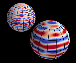
Remarkably, the minimal GNS model studied below permits non-trivial analytical solutions. Exact stationary solutions reported previously include three-dimensional Beltrami flows (Słomka & Dunkel Reference Słomka and Dunkel2017b) and two-dimensional (2-D) vortex lattices (Słomka & Dunkel Reference Słomka and Dunkel2017a). Furthermore, Mickelin et al. (Reference Mickelin, Słomka, Burns, Lecoanet, Vasil, Faria and Dunkel2018) recently explored GNS flows on 2-D curved surfaces and constructed stationary solutions for the case of a non-rotating sphere. Here, we generalize their work by deriving exact time-dependent solutions for GNS flows on rotating spheres, and by comparing them with direct numerical simulations (figure 1). We shall see that these exact GNS solutions correspond to Rossby waves propagating along alternating zonal jets, qualitatively similar to the large-scale flow patterns seen in planetary atmospheres (Heimpel, Aurnou & Wicht Reference Heimpel, Aurnou and Wicht2005; Schneider & Liu Reference Schneider and Liu2008).
Our study complements recent work which showed that non-equilibrium approaches can provide analytical insights into the dynamics of planetary flows (Delplace, Marston & Venaille Reference Delplace, Marston and Venaille2017) and atmospheres (Marston Reference Marston2012). In view of the recent successful application of phenomenological GNS models to active fluids (Dunkel et al. Reference Dunkel, Heidenreich, Drescher, Wensink, Bär and Goldstein2013; Słomka & Dunkel Reference Słomka and Dunkel2017b), the results below can also help advance the understanding of active matter propagation on curved surfaces (Sanchez et al. Reference Sanchez, Chen, Decamp, Heymann and Dogic2012; Zhang et al. Reference Zhang, Zhou, Rahimi and De Pablo2016; Henkes, Marchetti & Sknepnek Reference Henkes, Marchetti and Sknepnek2018; Nitschke, Reuther & Voigt Reference Nitschke, Reuther and Voigt2019) and in rotating frames (Löwen Reference Löwen2019).

Figure 1. Statistically stationary states of the normalized vorticity  $\unicode[STIX]{x1D701}\unicode[STIX]{x1D70F}$ from simulations (a–i) for
  $\unicode[STIX]{x1D705}\unicode[STIX]{x1D6EC}=1$ become more zonal (or banded) as the rotation rate
  $\unicode[STIX]{x1D6FA}\unicode[STIX]{x1D70F}$ increases (see also supplementary movie 1 available at https://doi.org/10.1017/jfm.2020.205). At the highest rotation rate
  $\unicode[STIX]{x1D6FA}\unicode[STIX]{x1D70F}=500$, the width of the alternating zonal jets is determined by the parameter
  $R/\unicode[STIX]{x1D6EC}$ that represents the ratio of the radius of the sphere and the diameter of the vortices forced by the GNS dynamics. The main characteristics of these flow patterns at high rotation rate are captured by spherical harmonics
  $Y_{\ell }^{0}(\unicode[STIX]{x1D703},\unicode[STIX]{x1D719})$ that solve the dynamical equations. Matching the length scale
  $R/\unicode[STIX]{x1D6EC}$ gives
  $\ell =6$ (j),
  $\ell =11$ (k) and
  $\ell =21$ (l) for
  $R/\unicode[STIX]{x1D6EC}=2$, 4 and 8, respectively.
2 Generalized Navier–Stokes model for linearly driven flow
After briefly reviewing the GNS equations in § 2.1, we derive the corresponding vorticity-stream function formulation on a rotating sphere in § 2.2.
2.1 Planar geometry
The GNS equations for an incompressible fluid velocity field  $\boldsymbol{v}(\boldsymbol{x},t)$ with pressure field
  $p(\boldsymbol{x},t)$ read (Słomka & Dunkel Reference Słomka and Dunkel2017a,Reference Słomka and Dunkelb)
 $$\begin{eqnarray}\displaystyle & \displaystyle \unicode[STIX]{x1D735}\boldsymbol{\cdot }\boldsymbol{v}=0, & \displaystyle\end{eqnarray}$$
 $$\begin{eqnarray}\displaystyle & \displaystyle \unicode[STIX]{x2202}_{t}\boldsymbol{v}+(\boldsymbol{v}\boldsymbol{\cdot }\unicode[STIX]{x1D735})\boldsymbol{v}=-\unicode[STIX]{x1D735}p+\unicode[STIX]{x1D735}\boldsymbol{\cdot }\unicode[STIX]{x1D748}, & \displaystyle\end{eqnarray}$$
where the higher-order stress tensor
 $$\begin{eqnarray}\displaystyle \unicode[STIX]{x1D748}=(\unicode[STIX]{x1D6E4}_{0}-\unicode[STIX]{x1D6E4}_{2}\unicode[STIX]{x1D6FB}^{2}+\unicode[STIX]{x1D6E4}_{4}\unicode[STIX]{x1D6FB}^{4})[\unicode[STIX]{x1D735}\boldsymbol{v}+(\unicode[STIX]{x1D735}\boldsymbol{v})^{\top }] & & \displaystyle\end{eqnarray}$$
accounts for both viscous damping and linear internal forcing. Transforming to Fourier space, the divergence of the stress tensor gives the dispersion relation
 $$\begin{eqnarray}\unicode[STIX]{x1D709}(k)=-k^{2}(\unicode[STIX]{x1D6E4}_{0}+\unicode[STIX]{x1D6E4}_{2}k^{2}+\unicode[STIX]{x1D6E4}_{4}k^{4}),\end{eqnarray}$$
 where  $k$ is the magnitude of the wave vector
  $\boldsymbol{k}$. Fixing hyperviscosity parameters
  $\unicode[STIX]{x1D6E4}_{0}>0$,
  $\unicode[STIX]{x1D6E4}_{4}>0$ and
  $\unicode[STIX]{x1D6E4}_{2}<-2\sqrt{\unicode[STIX]{x1D6E4}_{0}\unicode[STIX]{x1D6E4}_{4}}$, the growth rate
  $\unicode[STIX]{x1D709}(k)$ is positive between the two real roots
  $k_{-}$ and
  $k_{+}$. Hence, Fourier modes in the active band
  $k\in (k_{-},k_{+})$ are linearly unstable, corresponding to active energy injection into the fluid. The distance between the neutral modes
  $k_{\pm }$ defines the active bandwidth
  $\unicode[STIX]{x1D705}=k_{+}-k_{-}$.
Unstable bands are a universal feature of stress tensors exhibiting positive dispersion  $\unicode[STIX]{x1D709}(k)>0$ for some
  $k$. Polynomial GNS models of the type (2.1) were first studied in the context of seismic wave propagation (Beresnev & Nikolaevskiy Reference Beresnev and Nikolaevskiy1993; Tribelsky & Tsuboi Reference Tribelsky and Tsuboi1996) and can also capture essential statistical properties of dense microbial suspensions (Dunkel et al. Reference Dunkel, Heidenreich, Drescher, Wensink, Bär and Goldstein2013; Słomka & Dunkel Reference Słomka and Dunkel2017b). Since non-polynomial dispersion relations produce qualitatively similar flows (Słomka et al. Reference Słomka, Suwara and Dunkel2018a; Linkmann et al. Reference Linkmann, Boffetta, Marchetti and Eckhardt2019), we focus here on stress tensors of the generic polynomial form (2.1c).
Exact steady-state solutions of (2.1), corresponding to ‘zero-viscosity’ states, can be written as superpositions of modes  $\boldsymbol{k}$ with
  $|\boldsymbol{k}|=k_{+}$ or
  $|\boldsymbol{k}|=k_{-}$ (Słomka & Dunkel Reference Słomka and Dunkel2017b). Simulations of (2.1) with random initial conditions converge to statistically stationary states with highly dynamical vortical patterns that have a characteristic diameter
  ${\sim}\unicode[STIX]{x1D6EC}=\unicode[STIX]{x03C0}/k_{\ast }$, where
  $k_{\ast }$ is the most unstable wavenumber, corresponding to the maximum of
  $\unicode[STIX]{x1D709}(k)$ (Słomka et al. Reference Słomka, Suwara and Dunkel2018a; Słomka, Townsend & Dunkel Reference Słomka, Townsend and Dunkel2018b). Inverse energy transport in 2-D flows can bias the dominant vortex length scale towards larger values
  ${\sim}\unicode[STIX]{x03C0}/k_{-}$ (James et al. Reference James, Bos and Wilczek2018).
2.2 On a rotating sphere
We generalize planar 2-D GNS dynamics (2.1) to a sphere with radius  $R$ rotating at rate
  $\unicode[STIX]{x1D6FA}$. To this end, we adopt a corotating spherical coordinate system
  $(\unicode[STIX]{x1D703},\unicode[STIX]{x1D719})$ where
  $\unicode[STIX]{x1D703}$ is the colatitude and
  $\unicode[STIX]{x1D719}$ is the longitude. Following Mickelin et al. (Reference Mickelin, Słomka, Burns, Lecoanet, Vasil, Faria and Dunkel2018), we find the rotating GNS equations in vorticity-stream function form
 $$\begin{eqnarray}\displaystyle & \displaystyle \unicode[STIX]{x1D6FB}^{2}\unicode[STIX]{x1D713}=-\unicode[STIX]{x1D701}, & \displaystyle\end{eqnarray}$$
 $$\begin{eqnarray}\displaystyle & \displaystyle \unicode[STIX]{x2202}_{t}\unicode[STIX]{x1D701}+J(\unicode[STIX]{x1D713},\unicode[STIX]{x1D701})=F(\unicode[STIX]{x1D6FB}^{2}+4K)(\unicode[STIX]{x1D6FB}^{2}+2K)\unicode[STIX]{x1D701}+2\unicode[STIX]{x1D6FA}K\unicode[STIX]{x2202}_{\unicode[STIX]{x1D719}}\unicode[STIX]{x1D713}, & \displaystyle\end{eqnarray}$$
 $\unicode[STIX]{x1D701}$ is the vorticity in the rotating frame, and
  $K=1/R^{2}$ denotes the Gaussian curvature of the sphere. The active stress operator
  $F$ has the polynomial form
  $$\begin{eqnarray}F(x)=\unicode[STIX]{x1D6E4}_{0}-\unicode[STIX]{x1D6E4}_{2}x+\unicode[STIX]{x1D6E4}_{4}x^{2}.\end{eqnarray}$$
 The Laplacian  $\unicode[STIX]{x1D6FB}^{2}$ on the sphere is defined by
  $\unicode[STIX]{x1D6FB}^{2}=K(\cot \unicode[STIX]{x1D703}\unicode[STIX]{x2202}_{\unicode[STIX]{x1D703}}+\unicode[STIX]{x2202}_{\unicode[STIX]{x1D703}}^{2}+(\sin \unicode[STIX]{x1D703})^{-2}\unicode[STIX]{x2202}_{\unicode[STIX]{x1D719}}^{2})$ and
  $J(\unicode[STIX]{x1D713},\unicode[STIX]{x1D701})=K(\sin \unicode[STIX]{x1D703})^{-1}(\unicode[STIX]{x2202}_{\unicode[STIX]{x1D719}}\unicode[STIX]{x1D713}\unicode[STIX]{x2202}_{\unicode[STIX]{x1D703}}\unicode[STIX]{x1D701}-\unicode[STIX]{x2202}_{\unicode[STIX]{x1D703}}\unicode[STIX]{x1D713}\unicode[STIX]{x2202}_{\unicode[STIX]{x1D719}}\unicode[STIX]{x1D701})$ is the determinant of the Jacobian of the mapping
  $(R\unicode[STIX]{x1D719}\sin \unicode[STIX]{x1D703},R\unicode[STIX]{x1D703})\mapsto (\unicode[STIX]{x1D713},\unicode[STIX]{x1D701})$ from the tangent space of the sphere to the vectors
  $(\unicode[STIX]{x1D713},\unicode[STIX]{x1D701})$. The velocity components can be recovered from the stream function
  $\unicode[STIX]{x1D713}$ by
  $(v_{\unicode[STIX]{x1D719}},v_{\unicode[STIX]{x1D703}})=(-\unicode[STIX]{x2202}_{\unicode[STIX]{x1D703}}\unicode[STIX]{x1D713}/R,\unicode[STIX]{x2202}_{\unicode[STIX]{x1D719}}\unicode[STIX]{x1D713}/R\sin \unicode[STIX]{x1D703})$. In the non-rotating limit
  $\unicode[STIX]{x1D6FA}\rightarrow 0$, (2.3b) reduces to the model studied by Mickelin et al. (Reference Mickelin, Słomka, Burns, Lecoanet, Vasil, Faria and Dunkel2018). We note that (2.3b) is an internally forced extension of the unforced barotropic vorticity equation
  $\unicode[STIX]{x2202}_{t}\unicode[STIX]{x1D701}+J(\unicode[STIX]{x1D713},\unicode[STIX]{x1D701})=2\unicode[STIX]{x1D6FA}K\unicode[STIX]{x2202}_{\unicode[STIX]{x1D719}}\unicode[STIX]{x1D713}$ which has been widely studied in the earth sciences since the pioneering work of Charney, Fjörtoft & Neumann (Reference Charney, Fjörtoft and Neumann1950). Below we will show that the GNS model (2.3b) is analytically tractable, permitting exact travelling wave solutions that are close to the complex flow states observed in simulations.

Figure 2. The growth rate  $\unicode[STIX]{x1D6EF}$ of spherical harmonic modes
  $Y_{\ell }^{m}(\unicode[STIX]{x1D703},\unicode[STIX]{x1D719})$ in (2.5) plotted as a function of the wavenumber
  $\ell$. The parameters used to make this plot are
  $((\unicode[STIX]{x1D70F}/R^{2})\unicode[STIX]{x1D6E4}_{0},(\unicode[STIX]{x1D70F}/R^{4})\unicode[STIX]{x1D6E4}_{2},(\unicode[STIX]{x1D70F}/R^{6})\unicode[STIX]{x1D6E4}_{4})\simeq (1.43\times 10^{-2},-4.86\times 10^{-5},3.72\times 10^{-8})$ which correspond to
  $R/\unicode[STIX]{x1D6EC}=8$ and
  $\unicode[STIX]{x1D705}\unicode[STIX]{x1D6EC}=1$. The grey region indicates the active bandwidth where
  $\unicode[STIX]{x1D6EF}>0$ and energy is injected. Here,
  $\unicode[STIX]{x1D6EC}$ is the diameter of the vortices forced by the mode with the maximum growth rate
  $1/\unicode[STIX]{x1D70F}$, and
  $\unicode[STIX]{x1D705}$ is the active bandwidth i.e.
  $\unicode[STIX]{x1D705}=(\ell _{+}-\ell _{-})/R$ where
  $\unicode[STIX]{x1D6EF}(\ell _{\pm })=0$.
2.2.1 Dimensionless parameters
We assess the linear behaviour of (2.3b) using spherical harmonics  $Y_{\ell }^{m}(\unicode[STIX]{x1D703},\unicode[STIX]{x1D719})$, the eigenfunctions of the Laplacian operator on the sphere. With
  $\unicode[STIX]{x1D6FF}=K(\ell (\ell +1)-4)$, the linear growth rate of a spherical harmonic mode due to
  $F$ is
 $$\begin{eqnarray}\unicode[STIX]{x1D6EF}(\ell )=-(\unicode[STIX]{x1D6FF}+2K)F(-\unicode[STIX]{x1D6FF})=-(\unicode[STIX]{x1D6FF}+2K)(\unicode[STIX]{x1D6E4}_{0}+\unicode[STIX]{x1D6E4}_{2}\unicode[STIX]{x1D6FF}+\unicode[STIX]{x1D6E4}_{4}\unicode[STIX]{x1D6FF}^{2}),\end{eqnarray}$$
 which is the spherical analogue of (2.2). Using this relation, characteristic length and time scales,  $\unicode[STIX]{x1D6EC}$ and
  $\unicode[STIX]{x1D70F}$, for vortices forced by the GNS dynamics, along with the bandwidth of the forcing
  $\unicode[STIX]{x1D705}$, can be expressed in terms of
  $\unicode[STIX]{x1D6E4}_{0},\unicode[STIX]{x1D6E4}_{2},\unicode[STIX]{x1D6E4}_{4}$ and
  $R$ (figure 2 and appendix A). We use these scales to define the essential dimensionless parameters:
  $R/\unicode[STIX]{x1D6EC}$ is the ratio between the radius of the sphere and the characteristic vortex scale,
  $\unicode[STIX]{x1D705}\unicode[STIX]{x1D6EC}$ compares the forcing bandwidth to the characteristic vortex scale, and
  $\unicode[STIX]{x1D6FA}\unicode[STIX]{x1D70F}$ is dimensionless rotation rate. We note that since
  $\unicode[STIX]{x1D6EF}(\ell =1)=0$, the GNS dynamics do not force the
  $\ell =1$ mode which ensures that the total angular momentum is conserved (see appendix B). Finally, we define the Rossby number in terms of the characteristic flow speed
  ${\mathcal{U}}=\unicode[STIX]{x1D6EC}/\unicode[STIX]{x1D70F}$ and the dominant length scale
  ${\mathcal{L}}=\unicode[STIX]{x1D6EC}$ as
 $$\begin{eqnarray}Ro=\frac{{\mathcal{U}}}{\unicode[STIX]{x1D6FA}{\mathcal{L}}}=\frac{1}{\unicode[STIX]{x1D6FA}\unicode[STIX]{x1D70F}}.\end{eqnarray}$$
2.2.2  $\unicode[STIX]{x1D6FD}$-plane equations

When the vortical patterns are much smaller than the radius of the sphere ( $R/\unicode[STIX]{x1D6EC}\gg 1$), one can linearize around a reference colatitude
  $\unicode[STIX]{x1D703}_{0}$ to produce a local model. We define metric coordinates in the directions of increasing
  $\unicode[STIX]{x1D719}$ and decreasing
  $\unicode[STIX]{x1D703}$, respectively, by
  $x=R\sin (\unicode[STIX]{x1D703}_{0})\unicode[STIX]{x1D719}$ and
  $y=R(\unicode[STIX]{x1D703}_{0}-\unicode[STIX]{x1D703})$. In these coordinates the dynamical equations are
 $$\begin{eqnarray}\displaystyle & \displaystyle \unicode[STIX]{x1D6FB}_{c}^{2}\unicode[STIX]{x1D713}=-\unicode[STIX]{x1D701}, & \displaystyle\end{eqnarray}$$
 $$\begin{eqnarray}\displaystyle & \displaystyle \unicode[STIX]{x2202}_{t}\unicode[STIX]{x1D701}+J_{c}(\unicode[STIX]{x1D713},\unicode[STIX]{x1D701})=\unicode[STIX]{x1D6FB}_{c}^{2}F(\unicode[STIX]{x1D6FB}_{c}^{2})\unicode[STIX]{x1D701}+\unicode[STIX]{x1D6FD}\unicode[STIX]{x2202}_{x}\unicode[STIX]{x1D713}, & \displaystyle\end{eqnarray}$$
 $J_{c}(\unicode[STIX]{x1D713},\unicode[STIX]{x1D701})=\unicode[STIX]{x2202}_{y}\unicode[STIX]{x1D713}\unicode[STIX]{x2202}_{x}\unicode[STIX]{x1D701}-\unicode[STIX]{x2202}_{x}\unicode[STIX]{x1D713}\unicode[STIX]{x2202}_{y}\unicode[STIX]{x1D701}$ is the Cartesian Jacobian determinant,
  $\unicode[STIX]{x1D6FB}_{c}^{2}$ is the Cartesian Laplacian and the namesake
  $\unicode[STIX]{x1D6FD}$ parameter is given by
  $\unicode[STIX]{x1D6FD}=2\unicode[STIX]{x1D6FA}\sin \unicode[STIX]{x1D703}_{0}/R$. The
  $\unicode[STIX]{x1D6FD}$-plane equations preserve the effect of a varying Coriolis parameter
  $2\unicode[STIX]{x1D6FA}\cos \unicode[STIX]{x1D703}$ while simplifying the spatial operators. Rotational effects are accounted for by the term proportional to
  $\unicode[STIX]{x1D6FD}$.
2.2.3 Characteristic length and time scales
The turbulent outer layers of rotating stars and planets ubiquitously contain east–west (zonal) jets of various scales and strengths. Determining physical processes that generate and maintain these jets is an important problem in planetary science. A variety of theories have arisen describing jet formation, particularly on the  $\unicode[STIX]{x1D6FD}$-plane, including the arrest of the inverse cascade in rotating turbulence by nonlinear Rossby waves (Vallis & Maltrud Reference Vallis and Maltrud1993; Rhines Reference Rhines2006), and as a bifurcation in the statistical dynamics of the zonal flow as a function of the intensity of background homogeneous turbulence (Srinivasan & Young Reference Srinivasan and Young2012; Tobias & Marston Reference Tobias and Marston2013). These theories predict that jet formation may depend on a variety of length and time scales, such as the Rhines scale
  $L_{R}=\sqrt{{\mathcal{U}}/\unicode[STIX]{x1D6FD}}$, the scale at which small-scale forcing injecting energy at a rate
  $\unicode[STIX]{x1D716}$ is affected by rotation
  $L_{\unicode[STIX]{x1D716}}=(\unicode[STIX]{x1D716}/\unicode[STIX]{x1D6FD}^{3})^{1/5}$ (Galperin, Sukoriansky & Dikovskaya Reference Galperin, Sukoriansky and Dikovskaya2010), and the growth rate of unstable perturbations to the zonal flow in statistical models (Bakas, Constantinou & Ioannou Reference Bakas, Constantinou and Ioannou2019). The GNS model investigated here provides a simplified setting for examining the dynamics of jets by parameterizing the jet-formation physics, rather than attempting to resolve the details of the underlying formation processes. If one is interested in matching the effective GNS parameters to specific length and velocity scales of more detailed models, then guidance can be drawn from the observation that typical zonal jets in the GNS model have width
  ${\sim}\unicode[STIX]{x1D6EC}$ and root mean square velocity
  ${\sim}\unicode[STIX]{x1D6EC}\sqrt{\unicode[STIX]{x1D6FA}/\unicode[STIX]{x1D70F}}$ in the rotation dominated regime
  $\unicode[STIX]{x1D6FA}\unicode[STIX]{x1D70F}>1$.
3 Exact time-dependent solutions
Exact solutions can be constructed on the sphere as well as on the local  $\unicode[STIX]{x1D6FD}$-plane. Although not stable, these solutions will provide an intuitive understanding of the numerical results in § 4, similar to the role of exact coherent structures (Waleffe Reference Waleffe2001; Wedin & Kerswell Reference Wedin and Kerswell2004) in classical turbulence.
3.1 Global solutions
Exact time-dependent solutions to (2.3b) can be constructed as superpositions of normal spherical harmonic modes  $Y_{\ell }^{m}(\unicode[STIX]{x1D703},\unicode[STIX]{x1D719})$ as
 $$\begin{eqnarray}[\unicode[STIX]{x1D713}(\unicode[STIX]{x1D703},\unicode[STIX]{x1D719},t),\unicode[STIX]{x1D701}(\unicode[STIX]{x1D703},\unicode[STIX]{x1D719},t)]=[1,\ell _{\pm }(\ell _{\pm }+1)](\unicode[STIX]{x1D713}_{j}(\unicode[STIX]{x1D703})+\unicode[STIX]{x1D713}_{w}(\unicode[STIX]{x1D703},\unicode[STIX]{x1D719},t)),\end{eqnarray}$$
with
 $$\begin{eqnarray}\unicode[STIX]{x1D713}_{j}(\unicode[STIX]{x1D703})={\mathcal{A}}_{0}Y_{\ell _{\pm }}^{0}(\unicode[STIX]{x1D703}),\quad \unicode[STIX]{x1D713}_{w}(\unicode[STIX]{x1D703},\unicode[STIX]{x1D719},t)=\text{Re}\left[\mathop{\sum }_{m=1}^{\ell _{\pm }}{\mathcal{A}}_{m}Y_{\ell _{\pm }}^{m}(\unicode[STIX]{x1D703},\unicode[STIX]{x1D719})\exp (-\text{i}\unicode[STIX]{x1D70E}_{m}t)\right],\end{eqnarray}$$
 where  ${\mathcal{A}}_{m}$ for
  $m=0,1,\ldots$ are constants,
  $\ell _{\pm }$ are the roots of
 $$\begin{eqnarray}F(-\ell _{\pm }(\ell _{\pm }+1)+4)=0\end{eqnarray}$$
 and  $\unicode[STIX]{x1D70E}_{m}$ satisfies the dispersion relation
 $$\begin{eqnarray}c_{p}^{\unicode[STIX]{x1D719}}=\frac{\unicode[STIX]{x1D70E}_{m}}{m}=\frac{-2\unicode[STIX]{x1D6FA}}{\ell _{\pm }(\ell _{\pm }+1)}.\end{eqnarray}$$
 These solutions to (2.3b) are possible because the Jacobian determinant  $J$ vanishes if the stream function is a superposition of spherical harmonics
  $Y_{\ell }^{m}$ with fixed
  $\ell$. We choose
  $\ell$ to be one of the roots of the polynomial
  $F$ given in (3.3). Equation (3.4) describes the dispersion of normal-mode Rossby–Haurwitz waves (Hoskins Reference Hoskins1973; Lynch Reference Lynch2009; Madden Reference Madden2018). These are well known solutions of the barotropic vorticity equation (Thompson Reference Thompson1982) and propagate in the direction opposite to the sphere’s rotation with phase speed
  $c_{p}^{\unicode[STIX]{x1D719}}$. Overall, the exact solutions in (3.1) are a combination of time-independent zonal jets (
 $\unicode[STIX]{x1D713}_{j}$) and time-varying Rossby–Haurwitz waves (
 $\unicode[STIX]{x1D713}_{w}$). The time-independent zonal jets are spherical harmonics
  $Y_{\ell }^{0}(\unicode[STIX]{x1D703})$ which consist of alternating crests and troughs. A selection of such modes corresponding to different
  $\ell$s are shown in figure1(j–l).
3.2 $\unicode[STIX]{x1D6FD}$-plane solutions

Similar to the procedure on the full sphere, exact solutions to (2.7b) can be constructed by considering superpositions of Fourier modes with wave vectors  $\boldsymbol{k}$ that correspond to the neutral modes of the pattern-forming operator. Hence, the exact solutions are
 $$\begin{eqnarray}[\unicode[STIX]{x1D713}(x,y,t),\unicode[STIX]{x1D701}(x,y,t)]=[1,k_{\pm }^{2}](\unicode[STIX]{x1D713}_{j}(y)+\unicode[STIX]{x1D713}_{w}(x,y,t)),\end{eqnarray}$$
with
 $$\begin{eqnarray}\unicode[STIX]{x1D713}_{j}(y)=\text{Re}[{\mathcal{A}}_{0}\exp (\text{i}k_{\pm }y)],\quad \unicode[STIX]{x1D713}_{w}(x,y,t)=\text{Re}\left[\mathop{\sum }_{|\boldsymbol{k}|=k_{\pm }}{\mathcal{A}}_{\boldsymbol{k}}\exp (\text{i}(\boldsymbol{k}\boldsymbol{\cdot }\boldsymbol{x}-\unicode[STIX]{x1D70E}_{\boldsymbol{k}}t))\right],\end{eqnarray}$$
 where  ${\mathcal{A}}_{\boldsymbol{k}}$ are constants,
  $k_{\pm }$ are the positive roots of
  $F(-k_{\pm }^{2})=0$, and
  $\unicode[STIX]{x1D70E}_{\boldsymbol{k}}$ satisfies the Rossby-wave dispersion relation (Pedlosky Reference Pedlosky2003)
 $$\begin{eqnarray}c_{p}^{x}=\frac{\unicode[STIX]{x1D70E}_{\boldsymbol{k}}}{k_{x}}=\frac{-\unicode[STIX]{x1D6FD}k_{x}}{|\boldsymbol{k}|^{2}}.\end{eqnarray}$$
 Here again, solutions are a combination of a time-independent zonal flow ( $\unicode[STIX]{x1D713}_{j}(y)$) and time-varying Rossby waves (
 $\unicode[STIX]{x1D713}_{w}(x,y,t)$). For the parameters at which the
  $\unicode[STIX]{x1D6FD}$-plane approximation holds, the expression for the phase speed (3.7) provides an explicit dependence on the colatitude
  $\unicode[STIX]{x1D703}$ through the parameter
  $\unicode[STIX]{x1D6FD}=2\unicode[STIX]{x1D6FA}\sin \unicode[STIX]{x1D703}_{0}/R$. The dynamics at the poles are similar to those on a non-rotating flat plane and the non-inertial effects matter the most at the equator.
4 Simulations
Direct numerical simulations of (2.3b) were performed using a spectral code based on the open-source Dedalus framework (Burns et al. Reference Burns, Vasil, Oishi, Lecoanet and Brown2019). The code uses a pseudo-spectral method with a basis of spin-weighted spherical harmonics (Lecoanet et al. Reference Lecoanet, Vasil, Burns, Brown and Oishi2019; Vasil et al. Reference Vasil, Lecoanet, Burns, Oishi and Brown2019); see the appendix of Mickelin et al. (Reference Mickelin, Słomka, Burns, Lecoanet, Vasil, Faria and Dunkel2018). A spectral expansion with a cutoff  $\ell _{max}=256$ suffices to obtain converged solutions. The simulations are initialized with a random stream function and evolved from time
  $t/\unicode[STIX]{x1D70F}=0$ to
  $t/\unicode[STIX]{x1D70F}=50$. In all simulations, we vary the parameters
  $R/\unicode[STIX]{x1D6EC}$ and
  $\unicode[STIX]{x1D6FA}\unicode[STIX]{x1D70F}$ for fixed dimensionless bandwidth
  $\unicode[STIX]{x1D705}\unicode[STIX]{x1D6EC}=1$. Narrow-band driving with
  $\unicode[STIX]{x1D705}\unicode[STIX]{x1D6EC}\ll 1$ leads to ‘burst’ dynamics (Mickelin et al. Reference Mickelin, Słomka, Burns, Lecoanet, Vasil, Faria and Dunkel2018) whereas broad-band driving
  $\unicode[STIX]{x1D705}\unicode[STIX]{x1D6EC}\gg 1$ leads to classical turbulence (Frisch Reference Frisch1995). The simulations settle onto statistically stationary flow states after initial relaxation periods during which the active stresses continuously inject energy until the forcing and dissipation balance. The analysis below focuses on the statistically stationary states.
Figure 1(a–i) shows snapshots of the dimensionless relative vorticity  $\unicode[STIX]{x1D701}\unicode[STIX]{x1D70F}$ for a range of
  $R/\unicode[STIX]{x1D6EC}$ and
  $\unicode[STIX]{x1D6FA}\unicode[STIX]{x1D70F}$ at
  $t/\unicode[STIX]{x1D70F}=15$. In the non-rotating case
  $\unicode[STIX]{x1D6FA}\unicode[STIX]{x1D70F}=0$, we attain solutions akin to those obtained by Mickelin et al. (Reference Mickelin, Słomka, Burns, Lecoanet, Vasil, Faria and Dunkel2018). When the dimensionless rotation rate
  $\unicode[STIX]{x1D6FA}\unicode[STIX]{x1D70F}$ is increased, the flow becomes zonal, that is, the
  $\unicode[STIX]{x1D719}$-variation in the vorticity field decreases. At the highest rotation rate
  $\unicode[STIX]{x1D6FA}\unicode[STIX]{x1D70F}=500$, the vorticity field contains alternating bands of high and low vorticity with a characteristic width. For comparison, we plot the steady-state solutions
  $Y_{\lceil \ell _{-}\rceil }^{0}(\unicode[STIX]{x1D703})$, where
  $\lceil \cdot \rceil$ is the ceiling function, in figure 1(j–l). This corresponds to the smallest
  $\ell$ inside the active band. The formation of zonal flows in our model is consistent with the view (Parker & Krommes Reference Parker and Krommes2013; Galperin & Read Reference Galperin and Read2019) that such flow structures can be described within a generic pattern formation framework.

Figure 3. Data from steady-state solutions at  $t/\unicode[STIX]{x1D70F}=15$ for the highest rotation rate
  $\unicode[STIX]{x1D6FA}\unicode[STIX]{x1D70F}=500$. The rows correspond to
  $R/\unicode[STIX]{x1D6EC}=2$ (a–d), 4 (e–h) and 8 (i–l). Panels (a,e,i) show Mercator projections of the dimensionless vorticity
  $\unicode[STIX]{x1D701}\unicode[STIX]{x1D70F}$. Panels (b,f,j) show the zonal-mean azimuthal velocities
  $\langle v_{\unicode[STIX]{x1D719}}\rangle _{\unicode[STIX]{x1D719}}/(R/\unicode[STIX]{x1D70F})$. Panels (c,g,k) show spherical harmonic decomposition of dimensionless vorticity
  $\unicode[STIX]{x1D701}\unicode[STIX]{x1D70F}$ with marker size indicating amplitude and colour indicating phase. All plots indicate the existence of dominant zonal jets with
  $m=0$ and
  $\ell$s within the active band indicated in grey. These modes are close to the exact solutions in figure 1(j–l). Panels (d,h,l) show time variation of the energy of all the modes (black), active
  $m=0$ modes (red) and all other modes (green); the energy contained in the active
  $m=0$ accounts for most of the total energy in the statistically stationary state. See also supplementary movie 2.
To better visualize the banded solutions for high rotation rates, we plot Mercator projections of the vorticity in figure 3(a,e,i). The banded nature of the vorticity is also reflected in the alternating structure of the mean azimuthal velocity  $\langle v_{\unicode[STIX]{x1D719}}\rangle _{\unicode[STIX]{x1D719}}$ in figure 3(b,f,j). The predominant scales in the flow field can be measured using the spherical harmonic decomposition of the relative vorticity. Since
  $\unicode[STIX]{x1D701}\unicode[STIX]{x1D70F}$ is a real field, we plot only the coefficients with positive
  $m$ in panels (c,g,k). The largest modes have
  $m=0$ with
  $\ell$ values in the active band of the GNS model (indicated in grey). Figure 3(d–l) shows the total energy and the energy contained in the active
  $m=0$ modes as a function of time, calculated from the spherical harmonic coefficients as
 $$\begin{eqnarray}\frac{E(t)}{R^{2}/\unicode[STIX]{x1D70F}^{2}}=\frac{\unicode[STIX]{x1D70F}^{2}}{R^{2}}\mathop{\sum }_{m,\ell \neq 0}E_{m,\ell }(t)=\frac{1}{2}\mathop{\sum }_{m,\ell \neq 0}\frac{|\unicode[STIX]{x1D70F}\hat{\unicode[STIX]{x1D701}}_{m,\ell }(t)|^{2}}{R^{2}\ell (\ell +1)}.\end{eqnarray}$$
 After the initial relaxation phase, when the energy injection balances the energy dissipation, the total energy in the system fluctuates around a statistical mean. The active  $m=0$ modes carry most of the total energy, implying that the bulk dynamics are dominated by these few modes. This also explains the bandedness of the flow patterns since spherical harmonics with
  $m=0$ do not vary with the azimuthal angle
  $\unicode[STIX]{x1D719}$; see figure 1(j–l). Time-averaged energy spectra of the statistically steady states are plotted in figure 4. The energy shows a clear peak within the active bandwidth further suggesting that the active modes carry most of the total energy.

Figure 4. Energy spectra for (a)  $R/\unicode[STIX]{x1D6EC}=2$, (b)
  $R/\unicode[STIX]{x1D6EC}=4$ and (c)
  $R/\unicode[STIX]{x1D6EC}=8$. The grey shaded region indicates the active bandwidth where the spectra show a peak. The spectra for
  $(R/\unicode[STIX]{x1D6EC},\unicode[STIX]{x1D6FA}\unicode[STIX]{x1D70F})=(4,250)$, (4, 500) and (8, 500) have been obtained from an ensemble average of 10 simulations with random initial conditions.

Figure 5. Phase speed of the spherical harmonic modes  $(\ell ,m)$ in the forcing bandwidth, normalized by the analytical phase speed in (3.4), for
  $\unicode[STIX]{x1D6FA}\unicode[STIX]{x1D70F}=500$ and different values of
  $R/\unicode[STIX]{x1D6EC}$. The dotted line indicates the value 1 for comparison.

Figure 6. (a–d) Time–space diagrams of the deviation of vorticity,  $\unicode[STIX]{x1D701}-\langle \unicode[STIX]{x1D701}\rangle$, where
  $\langle \cdot \rangle$ is the average over time and space, indicate that the phase speed of the westward propagating Rossby waves in the local
  $\unicode[STIX]{x1D6FD}$-plane changes with latitude. (e–l) Logarithm of the power spectral density,
  $S=|\unicode[STIX]{x1D70F}\hat{\unicode[STIX]{x1D701}}(k_{x},\unicode[STIX]{x1D70E})|^{2}$, where
  $\hat{\unicode[STIX]{x1D701}}$ is the discrete Fourier transform, at different northern (e–h) and southern (i–l) latitudes. The grey regions indicate the forcing bandwidth with
  $k_{-}<|k_{x}|<k_{+}$ justifying the rapid decay of the power spectral density for
  $|k_{x}|>k_{+}$. The white lines in each panel show the analytical dispersion relation from (3.7) with
  $|\boldsymbol{k}|=k_{+}$ and
  $|\boldsymbol{k}|=k_{-}$; the one with the steeper slope corresponds to
  $k_{-}$. These predictions capture the variance of power spectral density.
Strikingly, the statistically stationary states exhibit Rossby waves. For high rotation rates, the Rossby number  $Ro$ defined by (2.6) is
  $\ll 1$. Thus, we can directly compare the linear phase speed given by (3.4) with the slopes of the linear least squares fits to the phase evolution of the coefficients of vorticity
  $\hat{\unicode[STIX]{x1D701}}_{m,\ell }(t)$ from the simulations. The normalized phase speed of the modes for different values of
  $R/\unicode[STIX]{x1D6EC}$ and
  $\unicode[STIX]{x1D6FA}\unicode[STIX]{x1D70F}=500$ is shown in figure 5. The plotted modes have
  $\ell$ in the active bandwidth, corresponding to the grey regions in figure 3(c,g,k). The phase speed of the modes from the simulations are close to 1 when normalized by the analytical prediction (figure 5), implying that the linearized theory captures the main characteristics of the nonlinear dynamics.
We also analyse the phase speed of the waves as a function of latitude. According to the dispersion relation in (3.7), the Rossby-wave phase speed  $c_{p}^{x}$ depends on the colatitude
  $\unicode[STIX]{x1D703}_{0}$ through
  $\unicode[STIX]{x1D6FD}=2\unicode[STIX]{x1D6FA}\sin \unicode[STIX]{x1D703}_{0}/R$. To check this prediction, we examine the local dynamics at a number of discrete latitudes (
 $\unicode[STIX]{x03C0}/2-\unicode[STIX]{x1D703}_{0}$) shown in figure 6(a–d) for
  $R/\unicode[STIX]{x1D6EC}=8$ and
  $\unicode[STIX]{x1D6FA}\unicode[STIX]{x1D70F}=500$ (the
  $\unicode[STIX]{x1D6FD}$-plane approximation is valid for these parameters). We show the 2-D discrete Fourier transform in time and spatial coordinate
  $x=R(\sin \unicode[STIX]{x1D703}_{0})\unicode[STIX]{x1D719}$ in panels (e–l) for the same northern and southern latitudes. The unstable modes lie within the forcing bandwidth or when
  $k_{-}<|\boldsymbol{k}|<k_{+}$. Hence, we plot the expected wave dispersion (3.7) making the approximations
  $|\boldsymbol{k}|\simeq k_{+}$ and
  $|\boldsymbol{k}|\simeq k_{-}$. This produces two analytical curves for
  $\unicode[STIX]{x1D70E}(k_{x})$ which are linear in
  $k_{x}$ for
  $k_{x}<k_{+}$. These curves capture the spread of the spectral power in the nonlinear dynamics at every latitude; see the white lines in figure 6(e–l). We subsequently infer that the nonlinear, statistically stationary states contain modes with phase speeds matching those of linear
  $\unicode[STIX]{x1D6FD}$-plane Rossby waves.
5 Conclusions
We have presented analytical and numerical solutions of generalized Navier–Stokes equations on a 2-D rotating sphere. This phenomenological model generalizes the widely studied barotropic vorticity equation by adding an internal forcing that injects energy within a fixed spectral bandwidth. We derived a family of exact time-dependent solutions to the GNS equations on the rotating sphere as well as in the local  $\unicode[STIX]{x1D6FD}$-plane. These solutions correspond to a superposition of zonal jets and westward-propagating Rossby waves. Simulations at high rotation rates confirm that the statistically stationary states are close to these exact solutions. We further showed that the phase speeds of waves in the simulations agree with those predicted for linear Rossby waves. Our results suggest that the GNS framework can serve as a useful minimal model for providing analytical insight into complex flows on rotating spheres, such as planetary atmospheres. It is possible to extend the GNS approach to incorporate more than one dominant length scale by modifying the functional form of the spectral forcing accordingly.
Acknowledgements
The authors thank J. Słomka, H. Ronellenfitsch, G. Flierl and B. Galperin for helpful discussions. The authors acknowledge G. Vasil and D. Lecoanet for the development of the numerical model used in Mickelin et al. (Reference Mickelin, Słomka, Burns, Lecoanet, Vasil, Faria and Dunkel2018), which also formed the basis of the numerical model in this work.
Declaration of interests
The authors report no conflict of interest.
Supplementary movies
Supplementary movies are available at https://doi.org/10.1017/jfm.2020.205.
Appendix A. Formulas for $\unicode[STIX]{x1D6EC},\unicode[STIX]{x1D70F}$ and $\unicode[STIX]{x1D705}$


For a sphere of radius  $R$,
$R$,  $(\unicode[STIX]{x1D6EC},\unicode[STIX]{x1D70F},\unicode[STIX]{x1D705})$ are related to
  $(\unicode[STIX]{x1D6E4}_{0},\unicode[STIX]{x1D6E4}_{2},\unicode[STIX]{x1D6E4}_{4})$ by (Mickelin et al. Reference Mickelin, Słomka, Burns, Lecoanet, Vasil, Faria and Dunkel2018) the following:
 $$\begin{eqnarray}\displaystyle & \displaystyle \unicode[STIX]{x1D6EC}=\frac{2\unicode[STIX]{x03C0}R}{2\sqrt{{\displaystyle \frac{17}{4}}-{\displaystyle \frac{\unicode[STIX]{x1D6E4}_{2}}{2\unicode[STIX]{x1D6E4}_{4}}}R^{2}}-1}, & \displaystyle\end{eqnarray}$$
 $$\begin{eqnarray}\displaystyle & \displaystyle \unicode[STIX]{x1D70F}=\left[\left(\frac{\unicode[STIX]{x1D6E4}_{2}}{2\unicode[STIX]{x1D6E4}_{4}}-\frac{2}{R^{2}}\right)\left(\unicode[STIX]{x1D6E4}_{0}-\frac{\unicode[STIX]{x1D6E4}_{2}^{2}}{4\unicode[STIX]{x1D6E4}_{4}}\right)\right]^{-1}, & \displaystyle\end{eqnarray}$$
 $$\begin{eqnarray}\displaystyle & \displaystyle \unicode[STIX]{x1D705}=\left(\frac{17}{2R^{2}}-\frac{\unicode[STIX]{x1D6E4}_{2}}{\unicode[STIX]{x1D6E4}_{4}}-2\sqrt{\frac{17^{2}}{16R^{4}}-\frac{17}{4R^{2}}\frac{\unicode[STIX]{x1D6E4}_{2}}{\unicode[STIX]{x1D6E4}_{4}}+\frac{\unicode[STIX]{x1D6E4}_{0}}{\unicode[STIX]{x1D6E4}_{4}}}\right)^{1/2}. & \displaystyle\end{eqnarray}$$
 Letting  $R\rightarrow \infty$ in (A 1), one obtains for the planar case (Słomka & Dunkel Reference Słomka and Dunkel2017b)
 $$\begin{eqnarray}\unicode[STIX]{x1D6EC}=\unicode[STIX]{x03C0}\sqrt{\frac{2\unicode[STIX]{x1D6E4}_{4}}{-\unicode[STIX]{x1D6E4}_{2}}},\quad \unicode[STIX]{x1D70F}=\left[\frac{\unicode[STIX]{x1D6E4}_{2}}{2\unicode[STIX]{x1D6E4}_{4}}\left(\unicode[STIX]{x1D6E4}_{0}-\frac{\unicode[STIX]{x1D6E4}_{2}^{2}}{4\unicode[STIX]{x1D6E4}_{4}}\right)\right]^{-1},\quad \unicode[STIX]{x1D705}=\left(-\frac{\unicode[STIX]{x1D6E4}_{2}}{\unicode[STIX]{x1D6E4}_{4}}-2\sqrt{\frac{\unicode[STIX]{x1D6E4}_{0}}{\unicode[STIX]{x1D6E4}_{4}}}\right)^{1/2}.\end{eqnarray}$$
Appendix B. Total angular momentum
Taking the surface mass density to be 1, the total angular momentum is given by
 $$\begin{eqnarray}\displaystyle M(t) & = & \displaystyle \int _{0}^{\unicode[STIX]{x03C0}}\int _{0}^{2\unicode[STIX]{x03C0}}R\sin \unicode[STIX]{x1D703}v_{\unicode[STIX]{x1D719}}\,\text{d}A=\int _{0}^{\unicode[STIX]{x03C0}}\int _{0}^{2\unicode[STIX]{x03C0}}R^{3}\sin ^{2}\unicode[STIX]{x1D703}v_{\unicode[STIX]{x1D719}}\,\text{d}\unicode[STIX]{x1D719}\,\text{d}\unicode[STIX]{x1D703}\nonumber\\ \displaystyle & = & \displaystyle \int _{0}^{\unicode[STIX]{x03C0}}\int _{0}^{2\unicode[STIX]{x03C0}}R^{3}\sin ^{2}\unicode[STIX]{x1D703}(-\unicode[STIX]{x2202}_{\unicode[STIX]{x1D703}}\unicode[STIX]{x1D713}/R)\,\text{d}\unicode[STIX]{x1D719}\,\text{d}\unicode[STIX]{x1D703}=-R^{2}\int _{0}^{\unicode[STIX]{x03C0}}\int _{0}^{2\unicode[STIX]{x03C0}}\sin ^{2}\unicode[STIX]{x1D703}\unicode[STIX]{x2202}_{\unicode[STIX]{x1D703}}\unicode[STIX]{x1D713}\,\text{d}\unicode[STIX]{x1D719}\,\text{d}\unicode[STIX]{x1D703}.\quad\end{eqnarray}$$
 Applying integration by parts for the  $\unicode[STIX]{x1D703}$-integral gives
 $$\begin{eqnarray}\displaystyle M(t) & = & \displaystyle -R^{2}\int _{0}^{2\unicode[STIX]{x03C0}}\left\{\int _{0}^{\unicode[STIX]{x03C0}}\sin ^{2}\unicode[STIX]{x1D703}\unicode[STIX]{x2202}_{\unicode[STIX]{x1D703}}\unicode[STIX]{x1D713}\,\text{d}\unicode[STIX]{x1D703}\right\}\text{d}\unicode[STIX]{x1D719}\nonumber\\ \displaystyle & = & \displaystyle -R^{2}\int _{0}^{2\unicode[STIX]{x03C0}}\left\{[\sin ^{2}\unicode[STIX]{x1D703}\unicode[STIX]{x1D713}]_{0}^{\unicode[STIX]{x03C0}}-\int _{0}^{\unicode[STIX]{x03C0}}2\sin \unicode[STIX]{x1D703}\cos \unicode[STIX]{x1D703}\unicode[STIX]{x1D713}\,\text{d}\unicode[STIX]{x1D703}\right\}\text{d}\unicode[STIX]{x1D719}\nonumber\\ \displaystyle & = & \displaystyle 2R^{2}\int _{0}^{2\unicode[STIX]{x03C0}}\int _{0}^{\unicode[STIX]{x03C0}}\sin \unicode[STIX]{x1D703}\cos \unicode[STIX]{x1D703}\,\unicode[STIX]{x1D713}\,\text{d}\unicode[STIX]{x1D703}\,\text{d}\unicode[STIX]{x1D719}.\end{eqnarray}$$
 We may expand the stream function as  $\unicode[STIX]{x1D713}(\unicode[STIX]{x1D703},\unicode[STIX]{x1D719})=\sum _{\ell ,m}\hat{\unicode[STIX]{x1D713}}_{\ell }^{m}(t)Y_{\ell }^{m}(\unicode[STIX]{x1D703},\unicode[STIX]{x1D719})$. The
  $\unicode[STIX]{x1D719}$-integral survives only for
  $m=0$ and
  $Y_{\ell }^{0}(\unicode[STIX]{x1D703},\unicode[STIX]{x1D719})=P_{\ell }^{0}(\cos \unicode[STIX]{x1D703})$ where
  $P$ represents the associated Legendre polynomials. Also realizing that
  $P_{1}^{0}(\cos \unicode[STIX]{x1D703})=\cos \unicode[STIX]{x1D703}$, we get
 $$\begin{eqnarray}\displaystyle M(t)=4\unicode[STIX]{x03C0}R^{2}\mathop{\sum }_{\ell }\hat{\unicode[STIX]{x1D713}}_{\ell }^{0}(t)\left\{\int _{0}^{\unicode[STIX]{x03C0}}P_{1}^{0}(\cos \unicode[STIX]{x1D703})P_{\ell }^{0}(\cos \unicode[STIX]{x1D703})\sin \unicode[STIX]{x1D703}\,\text{d}\unicode[STIX]{x1D703}\right\}. & & \displaystyle\end{eqnarray}$$
Finally, using the orthogonality relation
 $$\begin{eqnarray}\int _{0}^{\unicode[STIX]{x03C0}}P_{k}^{m}(\cos \unicode[STIX]{x1D703})P_{\ell }^{m}(\cos \unicode[STIX]{x1D703})\sin \unicode[STIX]{x1D703}\,\text{d}\unicode[STIX]{x1D703}=\frac{2(\ell +m)!}{(2\ell +1)(\ell -m)!}\unicode[STIX]{x1D6FF}_{k,\ell },\end{eqnarray}$$
we obtain
 $$\begin{eqnarray}M(t)=\frac{8\unicode[STIX]{x03C0}}{3}R^{2}\hat{\unicode[STIX]{x1D713}}_{1}^{0}(t).\end{eqnarray}$$
 Following the results by Lynch (Reference Lynch2003), it can be shown that there is no contribution to  $\hat{\unicode[STIX]{x1D713}}_{1}^{0}(t)$ from any triad interactions that result from the nonlinear dynamics. To see this, we let
  $\hat{\unicode[STIX]{x1D713}}_{l_{\unicode[STIX]{x1D6FE}}}^{m_{\unicode[STIX]{x1D6FE}}}(t)=\hat{\unicode[STIX]{x1D713}}_{1}^{0}(t)$, which interacts with coefficients
  $\hat{\unicode[STIX]{x1D713}}_{\ell _{\unicode[STIX]{x1D6FC}}}^{m_{\unicode[STIX]{x1D6FC}}}$ and
  $\hat{\unicode[STIX]{x1D713}}_{\ell _{\unicode[STIX]{x1D6FD}}}^{m_{\unicode[STIX]{x1D6FD}}}$. For a non-vanishing triad interaction, the necessary conditions,
  $|\ell _{\unicode[STIX]{x1D6FC}}-\ell _{\unicode[STIX]{x1D6FD}}|<\ell _{\unicode[STIX]{x1D6FE}}=1$ and
  $\ell _{\unicode[STIX]{x1D6FC}}\neq \ell _{\unicode[STIX]{x1D6FD}}$, cannot be simultaneously satisfied for
  $\ell _{\unicode[STIX]{x1D6FE}}=1$. Additionally, equation (2.5) shows that the GNS forcing is zero for
  $\ell =1$. Thus,
  $\hat{\unicode[STIX]{x1D713}}_{1}^{0}(t)$ remains constant and the total angular momentum is conserved.


