3.1 Flight trajectory modelling

One of the initial studies that modelled the trajectory for fuel consumption optimisation^{(Reference Neuman and Kreindler1)} created an algorithm capable of calculating the minimum fuel consumption during the climb phase from 2,000ft to 10,000ft for long-haul flights (6–12h of flight). The authors derived a system of dynamic equations considering small angles of attack and trajectory, coordinated turns and absence of atmospheric winds, and also assumed that the weight of the aircraft remained constant. Approach altitude is considered above 2,000ft, and climb, approach and landing speeds are set for a commercial jet airliner. The authors concluded that the trajectories combined with latero-directional and longitudinal flight were optimal in terms of fuel consumption when there was little variation in altitude. Finally, the authors concluded that the amount of fuel that can be optimised during the climb and descent phase in the terminal area of the flight is small compared with the fuel spent during the cruise phase. Nevertheless, it is important to account for these costs in flight planning.

Moreover, Ref. (Reference Grimm, Well and Oberle2) sought to quantify the importance of the change in the aircraft weight of the aircraft due to fuel consumption by developing a model that took into account two different approaches: the first assuming the aircraft has constant weight, and the second considering weight decrease as fuel consumed. The authors used the Direct Multiple Shooting Method (DMSM). This method, which is used for optimising boundary constraints only in the state domain, consists basically of dividing the range at which solutions are searched into several smaller ranges. Because it is quite iterative, DMSM becomes heavy for processing systems such as four-dimensional (4D) path optimisation problems.

To design an optimal trajectory for a commercial aircraft, taking into account realistic constraints along the trajectory, Ref. (Reference Betts and Cramer3) applied the direct transcription method. The goal was to achieve results that met civil aviation safety standards. Aircraft aerodynamics and propulsion data were processed using a cubic spline product tensor, which was investigated for two different approaches through data interpolation and least squares taking into account the turning restrictions. This method may be fast because of the approach by cubic splines, but this is only an approximation. For a more accurate approach, the need for continuous derivation can complicate the results.

Also, in the context of of 4D trajectories optimisation, Ref. (Reference Hagelauer and Mora-Camino4) conducted a study in which they presented a method based on Dynamic Programming (DP), in the presence of various time constraints. A discrete formulation of the problem was proposed, and the optimisation problem was solved using a progressive DP framework. Processing time was decreased using neural networks to calculate the costs associated with each decision step in the search process. This method was called soft DP (SDP). Comparing this method with the one described in the previous paragraph, the authors concluded that the use of neural networks to calculate fuel consumption in each decision step reduced by 88.2% the time spent processing.

More recent work, Ref. (Reference Franco, Rivas and Valenzuela5), based on Ref. (Reference Neuman and Kreindler1), consisted of analysing the cruise fuel minimisation problem for a fixed altitude and arrival time as a simple optimisation problem. The objective of this work was to verify the influence of cruising altitude in the calculation of optimal trajectories, calculating the minimum fuel required. Results were presented for a Boeing 767-300ER. The authors concluded that, for higher altitude cruise levels, there is little influence on the Mach number variation with the aircraft weight. In fact, the highest fuel consumption optimisation rates are obtained at higher altitudes.

The flight phases in which an aircraft consumes more fuel are undoubtedly the climb and cruise. Reference (Reference Turgut and Rosen6) studied the relationship between fuel consumption and altitude variation during the descent phase for a commercial transport aircraft. To find approximate solutions, the authors used a Genetic Algorithm (GA) composed of five modules. In the first module, the features of the program are determined. The features relating to the GA program include population, iteration, crossover and mutation ratios and accuracy degree. Other features such as flight ID, range of observation data and minimum and maximum limits for variables are related to flight parameters. The new accuracy degree, according to the variable limits, is also determined in this module. In the second module, the genomes are ranked to the values of the actual count of each genome. At the end of this task, the genomes that have a zero value of actual counts are replaced by genomes which have a maximum actual count. Modules three and four involve codes that perform the tasks of crossover and mutation. In the fifth module, the outputs of the first iteration are recorded in a data set. The output having the best solution in terms of objective function is also recorded on another data set with the values for variables along with the results from the iterations. Within the modules, auxiliary tasks are also conducted, such as routines for checking the proper performance of crossover and mutation and to prevent the loss of the best output from the population after the tasks of crossover and mutation. After analysing the results, the authors concluded that the optimum fuel consumption values occur when, during descent, the aircraft is kept as long as possible at higher altitudes.

The work of Ref. (Reference Murrieta-Mendoza, Ruiz and Botez7) optimises the fuel burn of the vertical profile of a commercial aircraft. The airspace was modelled under the form of a unidirectional graph. The selection of waypoints where to execute the changes in altitudes that provided the most economical flight cost in terms of fuel burn was determined using the Particle Swarm Optimisation (PSO) algorithm.

To compute the flight cost, the flight trajectory is divided into equidistant segments of 20 nautical miles. The authors claim that, by doing so, it is possible to achieve a good compromise between accuracy and computation time. At the beginning of each segment, the model subtracts from the aircraft’s gross weight the fuel burned required to travel the previous segment; the ground speed is computed considering the wind speed, wind direction and temperature; linear interpolations are executed to compute the fuel flow or the fuel burn and the horizontal travelled distance.

Fuel burn was computed in two different ways, depending on the cruise regime: steady altitude or change of altitude. The total fuel burn is calculated by aggregating all the segments, taking into account, if necessary, the change of altitude cost.

The weather forecast was obtained from the model delivered by Environment Canada. The trajectories provided by the algorithm developed in this paper were compared against simple geodesic trajectories to validate their optimisation potential, and against flown trajectories.The authors claim that the results show that up to 6.5% of fuel burn can be saved comparing against simple trajectories, and up to 3.1% was optimised comparing against flown trajectories.

In the work of Ref. (Reference Hartjes, van Hellenberg Hubar and Visser8), a tool is developed that optimises the trajectories of multiple airliners that seek to join in formation to minimise overall fuel consumption or direct operating cost. When in formation, a discount factor is applied to simulate reduction in the induced drag of the trailing aircraft. Using the developed tool, a case study has been conducted pertaining to the assembly of two-aircraft formation flights across the North Atlantic.

The authors mention that the results of the various numerical experiments show that formation flight can lead to significant reductions in fuel consumption compared with flying solo, even when the original trip times are maintained, and that the performance and the characteristics of the flight formation mission – notably the location of rendezvous and splitting points – are affected when one aircraft seeking to join the formation suffers a departure delay.

A fuel flow rate model was developed in Ref. (Reference Oruc and Baklacioglu9) using flight altitude, True Air Speed (TAS) and fuel flow rate values obtained from B737-800 type passenger aircraft Flight Data Records (FDRs). In the model, fuel flow rate is achieved as a function of altitude and TAS. The fuel flow rate model uses a Cuckoo Search Algorithm (CSA) for the climbing phase of the flight. The CSA used in this study uses a combination of local and global search. The authors claim that this approach increases search richness and versatility, while using Lévy flights makes the search area more efficient.

3.2 Flight modelling using BADA

Several other studies have evaluated the benefits of continuous or optimised profile descents and climbs. In general terms, these works are based on flight paths obtained from airspace control agencies. These flight paths and other flight information are then used in conjunction with an aircraft performance model, such as Eurocontrol’s BADA⁽¹⁰⁾ to estimate fuel consumption and the flight altitude profile. BADA is an aircraft performance model which is based on the total energy model of the aircraft and can be considered as a reduced point-mass model.

In the work of Ref. (Reference Melby and Mayer11), the authors analysed trajectory data at 34 US airports in one day, focusing on the continuity of vertical flight profiles at air terminals and the benefits that could be achieved by implementing vertical orientation Performance-Based Navigation (PBN) procedures. For this, they applied a metric that considers the time in level flight during the descent or ascent to the trajectories. The time in level flight metric evaluated the time selected departure operations required to climb through 100ft of altitude. Similarly, the metric evaluated the average time selected arrival operations required to descend through 100ft of altitude. Fuel consumption estimates were made with a BADA-based model. The results show that operators could save $380 million annually and associated reductions in carbon dioxide emission gases of 850,000 metric tons with more efficient descent and climb profiles.

To estimate the benefits of continuous descents in congested airspace, Ref. (Reference Robinson12) developed a model that built trajectories from flight plans at eight air terminals in the United States over a period of 30 to 60 days (depending on the airport). The descent phase flight segments were identified, and two types of continuous descent trajectories were modelled. In the first, level flight segments were moved to higher altitudes and a distance-only constraint was applied to simulate non-congested airspace. In the second, the level flight segments were also moved to higher altitudes, but now with a time constraint, to simulate congested airspace. BADA was used in this work as well, and the results show that potential savings are sensitive to the size and diversity of traffic analysed (e.g. number of days, flights, aircraft mix, etc.).

In Ref. (Reference Knorr, Chen, Rose, Gulding, Enaud and Hegendoerfer13), in addition to continuous descents, cruising speed reductions are exploited to absorb delays. This is encouraged by the fact that much of the extra fuel consumed is related to aircraft sequencing problems at the terminal. The authors methodology was based on four principles: the first consisting of supporting the analysis of a large number of flights, without detailed wind or aircraft weight data; the second consisting of the use of surveillance data for position information; the third consisting of the use of BADA table for aircraft performance information; and the fourth consisting of the potential benefit expressed in terms of time and fuel. The results show that the potential for improvement at the terminals averages 3min per flight or 100kg of fuel. Reductions in cruising speed can save up to 30% of total extra fuel, compared with optimal trajectory.

Using similar techniques, Ref. (Reference Howell and Dean14) assesses the impact of the Federal Aviation Administration (FAA) initiatives on the US flight efficiency during the descent phase. For this purpose, flight path data were collected between the years 2010 and 2015. Potential fuel savings were calculated for each flight, identifying flight level segments in the descent phase, and comparing the total fuel burned on each flight level segment with the total fuel that would have been burned if all these flight level segments were moved to the cruise phase. The calculation for potential time savings followed the same method. BADA was used for aircraft fuel consumption estimates. The results show that there has been a significant improvement in fuel efficiency, especially in places where optimised profile descents have been adopted.

Though previous studies focus on the CCD phases, aircraft surface movements in airports have also been the focus of research. Reference (Reference Khadilkar and Balakrishnan15) built a model that, given the taxi trajectory (for example, from a surface surveillance system), can estimate the resultant fuel burn from observations of the aircraft’s position, velocity and acceleration during taxi. The authors used the Flight Data Recorder (FDR) measurements of key aircraft parameters. FDR archives belonging to an international airline, from over 2,300 flights in the year 2004, were used in this study and introduced into two linear models for estimation of the taxi-out fuel burn. The first model is based on an initial hypothesis consisting of number of stops and number of turns made by the aircraft, with total fuel burn on the ground considered a function of the taxi time. The second incorporates lessons learned from the first model, namely, that other factors might be more important determinants of fuel burn. The authors removed the number of stops and the number of turns from the regression, and instead added the number of acceleration events as an independent variable. The logic behind this decision was that fuel flow rates were seen to increase for aggressive starts from standstill, as opposed to gradual ones. The parameters of both models were calculated using least-squares regression. According to the authors, taxi time is the main driver of fuel consumption, in particular, presented with an accurate estimate of the fuel burn indexFootnote ¹, a good estimate of the fuel consumption of a surface trajectory can be obtained using just the taxi time.

In Ref. (Reference Ravizza, Atkin, Maathuis and Burke16), the authors have developed a prediction model that combines both airport layout and historic taxi time information within a multiple linear regression analysis, identifying the most relevant factors affecting the variability of taxi times for both arrivals and departures. The two main applications of this research are for total taxi time prediction and for use in a ground movement decision support system. The authors use multiple linear regression to find a function which could more accurately predict the taxi times than existing methods and concluded that the average speed between the gate and runway (and between the runway and gate) was found to be highly correlated with the taxi distance, with higher speeds being expected for longer distances. Arrivals had higher taxi speeds than departures, because of departure queues at the runway, and the quantity of traffic at the airport was also found to have a significant impact upon the average taxi speed, as identified by several variables in the resulting model. During taxi, the authors also concluded, the turning angle and the operating mode (which runways were in use) were also highly correlated with the average taxi speed. Reference (Reference Ravizza, Chen, Atkin, Stewart and Burke17) uses the same explanatory variables and shows an extensive analysis of different regression approaches for predicting taxi times at airports to demonstrate the performance of each. Six different approaches were analysed in detail: multiple linear regression, least median squares linear regression, support vector regression, M5 model trees, Mamdani fuzzy rule-based systems and Takagi–Sugeno–Kang (TSK) fuzzy rule-based systems.

In Ref. (Reference Chen, Weiszer, Locatelli, Ravizza, Atkin, Stewart and Burke18), the authors present a new Active Routing (AR) framework to model fuel consumption, with the aim of providing a more realistic, cost-effective, and environmentally friendly surface movement. The paper focuses on optimal speed profile generation using a physics-based aircraft movement model. The two modelling approaches were based in BADA and in the International Civil Aviation Organization (ICAO) engine emissions database, respectively. The authors tested the model for Manchester International Airport and concluded that the results reveal an apparent trade-off between fuel burn and taxi times irrespective of fuel consumption modelling approaches.

The aim of Ref. (Reference Gardi, Sabatini and Ramasamy19) is to review the current scientific knowledge regarding the optimisation of transport aircraft flight trajectories with respect to multiple and typically conflicting objectives arising from the inclusion of multiple environmental and operational criteria, and to deduce or infer all the useful notions for the development of algorithms that are specifically conceived for the implementation in novel Communication Navigation and Surveillance/Air Traffic Management (CNS/ATM) and Avionics (CNS+A) systems. The Multi-Objective Trajectory (MOTO) model proposed in this work consists of an optimisation process split between control inputs and state variables. From these two, the authors establish a network of relations between the aircraft’s engine thrust, fuel consumption, dynamics models and the atmosphere. These relations return the inputs for the emissions, noise and contrail models, which will return the values for the output and state variables. The authors conclude that MOTO algorithms have a clear potential to enable real-time planning and re-planning of more environmentally efficient and economically viable flight routes by simultaneously addressing the dynamic nature of both weather and air traffic conditions.

There are several approaches regarding fuel burn estimations. To compare them, the work of Ref. (Reference Enea, Fricke, Paglione and Bronsvoort20) summarises the collaboration between researchers from several globally recognised institutions to address the question of fidelity of fuel estimation. Interviews were conducted initially to categorise common elements that typical Air Traffic Management (ATM) studies share. An international team of fuel modellers was assembled to run their models on a common set of inputs. The outputs generated by these models were categorised using metrics on empirical trajectories and other operational data, including predicted fuel burn. The set of flights analysed for this study was recorded in June 2015 from various airports in the United States. The sample included flights with variable length, different origin–destination pairs, various aircraft types and for different days of the month of June 2015. Flights from 19 different days, 65 origin–destination pairs and 16 different aircraft types were selected. To present a meaningful cross-comparison of the fuel burn models evaluated, only the subset of common flights was used for this analysis. This subset represented the maximum number of flights with valid fuel and TOW predictions from all the models. There was wide variability in the observed fuel burn error across all models. The smallest median error was obtained with the DaliFootnote ² BADA 3 run with $-3.9$%, while the largest median error was observed for the Aircraft Fuel Evaluation Simulation Tool (AFEST)Footnote ³ run without known TOW, with $-13.1$%, the latter representing a deterioration from the AFEST run with known TOW that presented a median error of $-9.5$%, hence showing the impact of the initial TOW error. The authors concluded that even the highest fidelity model will significantly underperform if low-quality input data is provided. Thus, one of the results of this work is that fuel burn estimation models with different levels of complexity perform with different levels of accuracy.

To model the descent and approach to the destination airport, Ref. (Reference Glaser-Opitz, Labun, Budajová and Glaser-Opitz21) propose a landing system where this phase can be done more efficiently and safely using performance data based on terrain reference navigation from their own created terrain elevation database, based on radar altimeter measurements compared with the overflown terrain. The simulations were performed for a flight arriving at Kosice (KSC) airport, a Boeing 737-800 aircraft, and the descent trajectory was modelled with a BADA performance model as a continuous descent approach from a proposed merging point to the KSC runway. The descent procedure for this airport was designed in cooperation with professional pilots, and all simulations were created for KSC as a continuous descent approach; procedures, based on real world airline data in compliance with initial 4D (i4D) trajectory and proposed merging point. Based on mentioned models and simulations, the landing system prototype was developed, with BADA model-based trajectory prediction capability. The authors developed a client–server interface for testing and further research activities, which enabled the landing system prototype to communicate with the flight simulator and datalink communication simulator. Although the authors described the methods used to derive the landing system thoroughly, they did not make any explicit conclusions regarding its efficiency or safety.

In summary, the previous paragraphs describe several models that aim to model specific phases of a flight, such as ground movements or CCD phases. The methods range from solving differential equations to linear regression, but none of them conduct a complete analysis for a flight, from the departure to arriving gate.

4.1 Calculating ground distance and defining cruise altitude

Given the:

• $\phi_o$ latitude for the origin airport

• $\lambda_o$ longitude for the origin airport

• $\phi_d$ latitude for the destination airport

• $\lambda_d $ longitude for the destination airport

  (1) \begin{equation} \Delta\phi = \phi_d - \phi_o\end{equation}
  (2) \begin{equation} \Delta\lambda = \lambda_d - \lambda_o\end{equation}
  (3) \begin{equation} a = \sin^2 \left(\frac{\Delta\phi}{2}\right) + \cos(\phi_o)\times \cos(\phi_d) \times \sin^2\left(\frac{\Delta \lambda}{2}\right)\end{equation}
  and assuming that Earth is perfect sphere with a radius R of 6,378.137km, we can determine the physical distance d between the origin and destination airports using the haversine formula in Equation (4):
  (4) \begin{equation} d = 2 \times R \times a\tan \left( \frac{\sqrt{a}}{\sqrt{1 - a}} \right)\end{equation}

To avoid collisions between aircraft travelling in opposite directions, it is necessary to impose a vertical separation. The ICAOFootnote ⁴ semi-circular rule defines the available flight levels in the conventional airspace and also in the Reduced Vertical Separation Minima (RVSM) airspace when applicable between FL290 and FL410. The default worldwide semi-circular rule can be observed in Fig. 1 and is applied according the aircraft’s magnetic bearing: if this value is between $0^{\circ}$ and $179^{\circ}$ (eastbound flights), the flight level or altitude must be odd, i.e. FL310, FL330, FL350, etc., whereas if the aircraft has a magnetic bearing between $180^{\circ}$ and $359^{\circ}$ (westbound flights), the flight level must be even, i.e. FL320, FL340, FL360, etc.

Figure 1. ICAO cruising levels (RVSM). Source: ICAO.

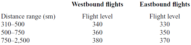
Based on the work of Ref. (Reference Pagoni and Psaraki-Kalouptsidi22), we define for our model in Table 1 the flight levels as a function of the distance intervals. Reference^{(Reference Pagoni and Psaraki-Kalouptsidi22)} noticed that short-haul flights present significant deviations in cruise altitude even for shorter distances and in their study adopt a distance increment of 250 statute milesFootnote ⁵ (sm) to present the data. On the other hand, longer flights tend to have a more homogeneous flight performance, and the distance increment is increased to 500sm. We will use an extended flight distance profile, although the one used by the authors, from 500sm to 2,500sm, was used to cover a wide spectrum of US domestic flight distances. Indeed, those flights comprise 87.4% of total passenger miles in 2012.

Table 1 Flight level for westbound and eastbound flights during cruise phase

4.2 Modelling taxi-out, take-off, approach, landing and taxi-in phases

For taxi-out, take-off, approach, landing and taxi-in phases, this paper uses the data set provided by the EMEPFootnote ⁶/EEAFootnote ⁷ air pollutant emission inventory guidebook 2016 1.A.3.a Aviation – Annex 5 – LTO emissions calculator 2016. The fuel burnt and emission data provided in this set are for supporting the European Union (EU) and the member states of the EEA in the maintenance and provision of European and national emission inventories. Fuel burn and emission data in this spreadsheet are modelled estimates and not absolute values. Where only one type of engine is associated with a particular aircraft type, it is the most common type of engine (as seen in Europe), or the best equivalent type of engine, for that aircraft type. Where several types of engine are associated with a particular aircraft type, the most common type of engine is highlighted.

The first part of our modelling will use the EMEP/EEA data set and consists of determining the duration and fuel flow for the taxi-out and take-off phases, on the basis of the type of the aircraft, origin airport and year. Since the ROADEF 2009 does not provide any information regarding the aircraft engine, we chose to use the most common aircraft engine. The mass of fuel burnt $M_{out}$ during the taxi-out phase is calculated using Equation (5):

(5) \begin{equation} M_{out} = T_{out} \times E_7 \times N_e\end{equation}

where $T_{out}$ is the taxi-out time (s), $E_7$ is the rate of fuel burn (kg/s/engine) during taxi-out and $N_e$ is the number of engines of the particular aircraft performing the flight. EMEP/EEA assumes that during the taxi-out phase the engine thrust is set to 7% following the ICAO convention. Similarly, the mass of fuel burnt $M_{off}$ during take-off is calculated using Equation (6):

(6) \begin{equation} M_{off} = T_{off} \times E_{100} \times N_e\end{equation}

where $T_{off}$ is the take-off time (s) and $E_{100}$ is the rate of fuel burn (kg/s/engine) during take-off. In this phase, EMEP/EEA assumes that during the take-off phase the engine thrust is set to 100% following the ICAO convention.

The mass of fuel burnt $M_{al}$ during the approach and landing phase is calculated using Equation (7):

(7) \begin{equation} M_{al} = T_{al} \times E_{30} \times N_e\end{equation}

where $T_{al}$ is the approach and landing time (s), and $E_{30}$ is the rate of fuel burn (kg/s/engine) during approach and landing. In this phase, EMEP/EEA assumes that during the take-off phase the engine thrust is set to 30% following the ICAO convention.

The mass of fuel burnt $M_{in}$ during the taxi-in phase is calculated using Equation (8):

(8) \begin{equation} M_{in} = T_{in} \times E_7 \times N_e\end{equation}

where $T_{in}$ is the taxi-in time (s), $E_7$ is the rate of fuel burn (kg/s/engine) during taxi-in and $N_e$ is the number of engines of the particular aircraft performing the flight. EMEP/EEA assumes that during the taxi-in phase the engine thrust is set to 7% following the ICAO convention.

4.3 Modelling climb descent and cruise phases

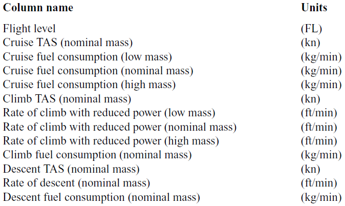
To model the CCD phases, we will use BADA Performance Table Files (PTF) for each specific aircraft. In Table 2, we present the performance data structure within the file.

Table 2 BADA performance data structure

To model the the CCD phases, we will use Newton’s equations of motion:

(9) \begin{equation} v = a \times t + v_0\end{equation}

(10) \begin{equation} r = r_0 + v_0 \times t + \frac{1}{2} \times a \times t^2\end{equation}

(11) \begin{equation} r = r_0 + \frac{1}{2} \times (v + v_0) \times t\end{equation}

(12) \begin{equation} v^2 = v_0^2 + 2 \times a \times (r - r_0)\end{equation}

(13) \begin{equation} r = r_0 + v \times t - \frac{1}{2}\times a \times t ^2\end{equation}

where $r_0$ is the initial position, r the final position, $v_0$ the initial velocity, v is the final velocity, a the acceleration and t is the time interval.

For the climb phase, to obtain the Rate Of Climb and Descent (ROCD) and fuel flow, we will be using the values for nominal mass level to avoid the problem of missing climb data for several aircraft models at high mass levels. During the climb phase, the model will interpolate between pairs of flight levels (current $FL_c$ and next $FL_n$ respectively), the pairs of values for true airspeed $(TAS_c, TAS_n)$, fuel flow $(f_{cc}, f_{cn})$ and ROCD $(R_c, R_n)$.

Figure 2 depicts the interpolation process during the climb phase between FL0 to FL5 and FL5 to FL10.

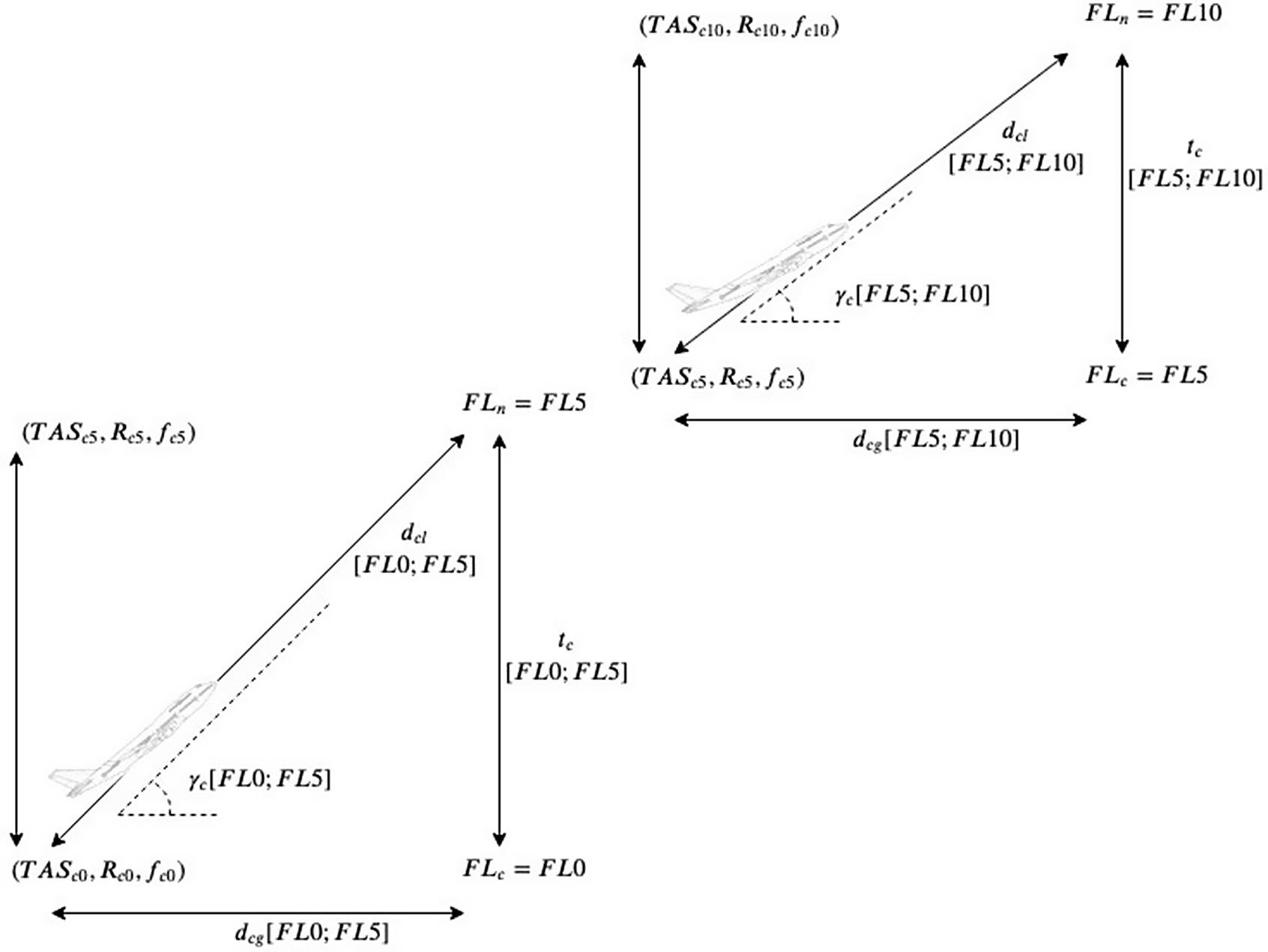
Figure 2. Climb between flight levels FL0 to FL5 and FL5 to FL10.

Since the ROCD consists of the variation of altitude with time, we consider it to be the aircraft’s vertical speed component. Since the ROCD changes with altitude, we proceed to obtain its rate of change with time. The latter consists of the vertical component of the aircraft’s acceleration $a_{cv}$, and it is calculated by interpolating between the current $(FL_c)$ and next $(FL_n)$ flight level, the ROCD $R_c$ and $R_n$, respectively. On the basis of Equation (12), the interpolation equation is expressed as follows:

(14) \begin{equation} a_{cv} = \frac{1}{2} \times \frac{R_n^2 -R_c^2}{FL_n - FL_c}\end{equation}

After determining the aircraft’s vertical acceleration, we can now determine, on the basis of Equation (9), the time $t_c$ the aircraft took to travel from $FL_c$ to $FL_n$:

(15) \begin{equation} t_{c} = \frac{R_n - R_c }{a_{cv}}\end{equation}

The longitudinal component of the aircraft’s acceleration $a_{cl}$ is determined on the basis of Equation (9), measuring the variation of TAS between the current and the next flight level, $TAS_c$ and $TAS_n$, respectively:

(16) \begin{equation} a_{cl} = \frac{TAS_n - TAS_c }{t_{c}}\end{equation}

The longitudinal distance $d_{cl}$ that the aircraft flew during the ascent between the current and next flight level can be calculated on the basis of Equation (11) and can thus be obtained by:

(17) \begin{equation} d_{cl} = TAS_c \times t_c + \frac{1}{2} \times a_{cl} \times t_c^2\end{equation}

The aircraft’s trajectory angle $\gamma_c$ is obtained by:

(18) \begin{equation} \gamma_{c} = \arcsin\left( \frac{FL_n - FL_c}{d_{cl}} \right)\end{equation}

The ground distance $d_{cg}$ is obtained projecting the longitudinal distance $d_{cl}$ on the horizontal plane:

(19) \begin{equation} d_{cg} = d_{cl} \times \cos(\gamma_c)\end{equation}

Finally, for the climb phase, we derive the amount of fuel consumed using a similar approach. We first calculate the variation of the fuel flow $F_{cf}$ during the time interval $t_c$, according to:

(20) \begin{equation} F_{cf} = \frac{f_{cn} - f{cc}}{t_c}\end{equation}

where $f_{cn}$ and $f_{cc}$ are the fuel flow for the next and current flight levels. The total amount of fuel consumed $C_c$ during the time interval $t_c$ is obtained using:

(21) \begin{equation} C_{c} = f_{cc} \times t_c + \frac{1}{2} \times F_{cf} \times t_c^2\end{equation}

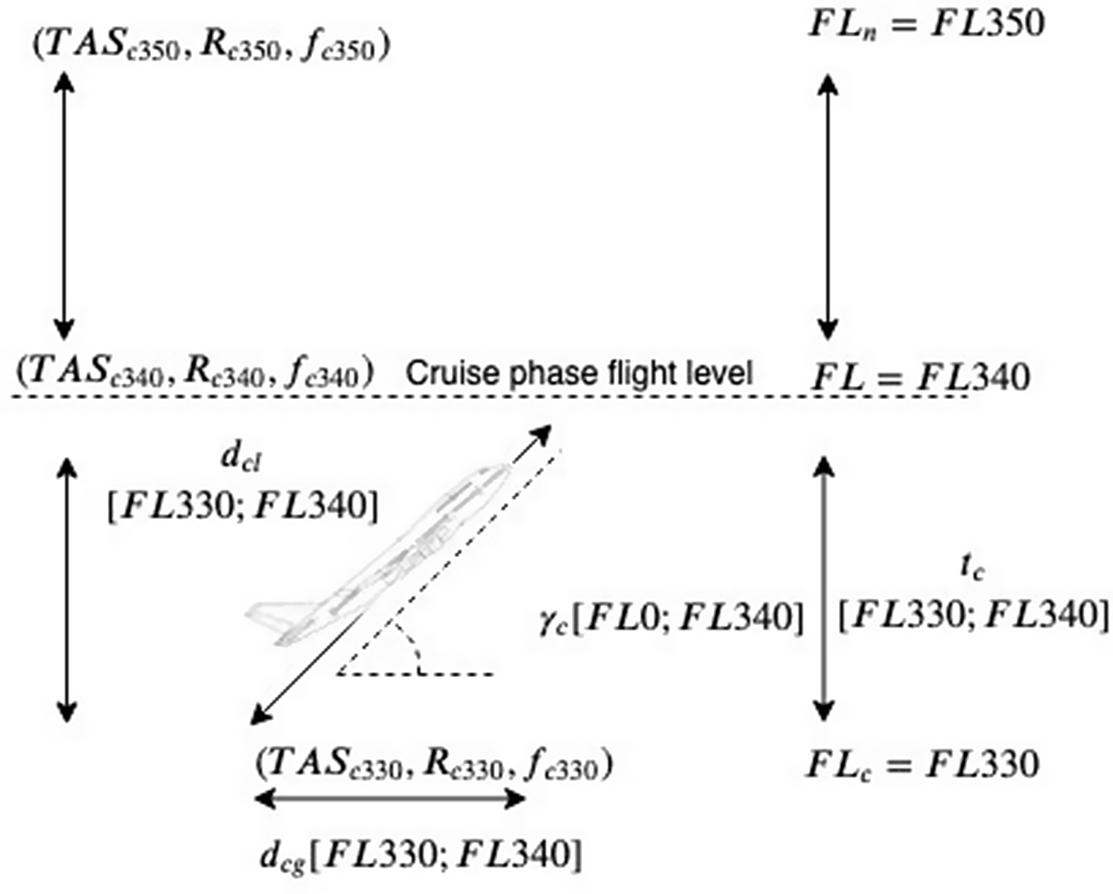
During the climb phase, the interpolation procedure will terminate when the aircraft reaches the cruise Flight Level (FL). For some aircraft models, there are no data points for the specific cruise FL; for instance, for an A320 that will cruise at FL340, the PTF only has data points ($TAS_c$, $R_c$ and $f_c$) for FL330 and FL350. In Fig. 3, we depict the interpolation between FL330 and FL340:

Figure 3. Climb between flight levels FL330 to FL340.

In the next part of our model, we will calculate for the descent phase the values of the vertical acceleration $a_{dv}$, time of descent $t_d$, longitudinal acceleration $a_{dl}$, longitudinal distance $d_{dl}$, aircraft’s trajectory angle $\gamma_d$, ground distance $d_{dg}$, fuel flow variation $F_{df}$ and total amount of consumed fuel $C_d$. The descent phase is symmetrical to the climb phase; thus, in the descent phase, we will interpolate between flight levels, starting at cruise altitude until 3,000ft (FL30), since from there on we will be using EMEP/EEA to model approach, landing and taxi-in. The reason for this procedure derives from the fact that the EMEP/EEA data set aggregates in a single-phase approach and landing.

Finally, for the cruise phase, we start by calculating the ground distance $d_{g}$ that needs to be covered using:

(22) \begin{equation} d_g = d - (d_{cg} - d_{dg})\end{equation}

To calculate the time $t_{cr}$ that it takes to fly the ground distance, we assume that its value is the same as the one the aircraft will travel. The value for the TAS can be obtained directly from the PTF if the cruise flight level is present. Otherwise, we will interpolate between the two pairs, lower and upper FL and lower and upper TAS. Thus, the cruise time $t_{cr}$ is obtained by:

(23) \begin{equation} t_{cr} = \frac{d_g}{TAS}\end{equation}

Similarly, the value for the fuel flow ($ \Phi $) during the cruise phase can be obtained directly from the PTF if the cruise flight level is present. Otherwise, we will interpolate between the two pairs, lower and upper FL and lower and upper $ \Phi $. Thus, the consumed fuel F during the cruise phase is obtained by:

(24) \begin{equation} F = \Phi \times t\end{equation}

With the final Equation (24), we achieve a complete integration of all phases of a flight. In the next section, we will calculate for each of them the start and end time, consumed fuel, start and end altitude and ground distance.