


1 Introduction
In this paper, we consider the class of non-negative distributions defined by the Mellin–Stieltjes convolution (Bingham et al., Reference Bingham, Goldie and Teugels1987) of two non-negative distributions G and H, given by
 $$F(x)\,{\equals}\,{\int}_0^\infty {G(x\,/\,s)dH(s)} ,\quad \quad x\geq 0$$
A distribution of the form (1.1) will be called a phase-type (PH) scale mixture if G is a (classical) PH distribution (cf. Latouche & Ramaswami, Reference Latouche and Ramaswami1999) and H is a proper non-negative distribution that we shall call the scaling distribution. A PH scale mixture distribution can be seen as the distribution of a random variable X:=S⋅Y, where S~H and Y~G; accordingly, S is referred as the scaling random variable. This terminology is also explained using conditional arguments: observe that (X|S=s)~G s , where G s (x):=G(x/s) corresponds to the distribution of the (scaled) random variable s⋅Y which is itself a PH distribution, so the distribution F can be thought as a mixture of the scaled PH distributions in {G s :s>0} with respect to the scaling distribution H.
Our motivation for studying the tail behaviour of PH scale mixtures is their use for approximating heavy-tailed distributions in risk applications (Bladt et al., Reference Bladt, Campillo Navarro and Nielsen2015a, Reference Bladt, Nielsen and Samorodnitsky2015b). To introduce such an approach, we shall first recall that the family of (classical) PH distributions, which corresponds to distributions of absorption times of Markov jump processes with one absorbing state and a finite number of transient states. The PH class is particularly attractive since it is tractable and possesses many desirable properties (densities, cumulative distributions, moments and integral transforms have closed-form expressions in terms of matrix exponentials; it is a closed class under scaling, finite mixtures and finite convolutions (cf. Assaf & Levikson, Reference Assaf and Levikson1982; Maier & O’Cinneide, Reference Maier and O’Cinneide1992). The PH class is popular for modelling purposes because it is dense in the non-negative distributions (cf. Asmussen, Reference Asmussen2003), so one could in principle approximate any non-negative distribution with an arbitrary precision. This classical approach has been widely studied and reliable methodologies for approximating non-negative distributions are already available (cf. Asmussen et al., Reference Asmussen, Nerman and Olsson1996).
However, distributions in the PH class are light-tailed and belong to the Gumbel domain of attraction exclusively (Kang & Serfozo, Reference Kang and Serfozo1999). Therefore, the PH class cannot correctly capture the characteristic behaviour of a heavy-tailed distribution in spite of its denseness. In fact, this approach may deliver unreliable approximations for important quantities of interest, such as the ruin probability of a Cramér–Lundberg risk process with heavy-tailed claim size distributions (Vatamidou et al., Reference Vatamidou, Adan, Vlasiou and Zwart2014). As an alternative, the PH class has been extended to distributions of absorption times having a countable number of transient states (this approach is attributed to Neuts, Reference Neuts1981). The later class, which goes under the name of infinite dimensional phase-type distributions (IDPH), is known to contain heavy-tailed distributions. Nevertheless, the IDPH class is no longer mathematically tractable and it is not fully documented yet (to the best of the authors’ knowledge, one of the few published references available outlining its mathematical properties is Shi et al. (Reference Shi, Guo and Liu1996); another reference of interest is Greiner et al. (Reference Greiner, Jobmann and Lipsky1999), who consider infinite mixtures of exponential distributions to approximate power-tailed distributions).
To address this issue, Bladt et al. (Reference Bladt, Campillo Navarro and Nielsen2015a, Reference Bladt, Nielsen and Samorodnitsky2015b) propose the use of PH scale mixtures having discrete scaling distributions to approximate heavy-tailed distributions. Such a class forms a structured subfamily of the IDPH class that contains the PH class, so it is trivially dense in the non-negative distributions. Two important advantages over the more general IDPH class are that the class of PH scale mixture distributions is mathematically tractable and that it contains a rich variety of heavy-tailed distributions.
The class of PH scale mixture distributions has great potential in applications in engineering, finance and specifically in insurance. As an example of the later, Bladt et al. (Reference Bladt, Campillo Navarro and Nielsen2015a, Reference Bladt, Nielsen and Samorodnitsky2015b) provide renewal results that can be applied to obtain exact expressions for the ruin probability of a classical Cramér–Lundberg risk process having claim sizes distributed according to a PH scale mixture distribution with discrete scaling. This approach is further explored in Peralta et al. (Reference Peralta, Rojas-Nandayapa, Xie and Yao2016), where a systematic methodology for approximating arbitrary heavy-tailed distributions via PH scale mixtures is provided; such a formulation provides simplified formulas for approximating ruin probabilities with arbitrary claim size distributions. Furthermore, Bladt & Rojas-Nandayapa (Reference Bladt and Rojas-Nandayapa2017) provide statistical inference procedures based on the expectation maximization algorithm to adjust PH scale mixtures to heavy-tailed data/distributions. Other references of interest that apply similar ideas to risk models include Hashorva et al. (Reference Hashorva, Pakes and Tang2010) and Vatamidou et al. (Reference Vatamidou, Adan, Vlasiou and Zwart2013).
In spite of the denseness and the mathematically tractability of the class of PH scale mixtures, the tail properties of the proposed class are not fully understood yet; this paper concentrates on this issue. In particular, a key aspect in the successful approximation of heavy-tailed distributions via PH scale mixtures is the appropriate selection of the scaling distribution. This paper focusses on the theoretical foundations justifying the selections made in some of the applications mentioned above, as well as on providing general guidelines for selecting appropriate scaling distributions. We collect and adapt some known results which are available in different contexts, and we prove new results that will allow us to provide a characterisation of the tail behaviour of PH scale mixtures, as well as a classification of their maximum domains of attraction. We expect our results to be useful for modelling purposes by providing a better understanding of the advantages and limitations of such an approach, as well as providing criteria for selecting appropriate scaling distributions for approximating general heavy-tailed distributions. Our results are summarised below.
First, we concentrate on classifying light- and heavy-tailed distributions. A PH scale mixture is heavy-tailed if and only if its scaling distribution has unbounded support. An interesting heuristic interpretation of this result is as follows: a PH random variable multiplied with a random variable S is heavy-tailed iff S has unbounded support. We provide a simple proof of this fact but we remark that a proof (unknown to us until recently) was already provided in a different context (cf. Su & Chen, Reference Su and Chen2006; Tang, Reference Tang2008).
Second, we focus on the maximum domains of attraction and subexponential properties of the class of PH scale mixtures. A classical result for the Fréchet case is Breiman’s Breiman (Reference Breiman1965) lemma, which implies that a PH scale mixture with a regularly varying scaling distribution remains regularly varying with the same index (hence subexponential). An analogue closure property exists for the class of Weibullian distributions (Arendarczyk & Dębicki, Reference Arendarczyk and Dębicki2011). In addition, we investigate analogue results for scaling distributions in the Gumbel domain of attraction. We show that if a certain higher order derivative of the Laplace–Stieltjes transform of the reciprocal of the scaling random variable
 $${\cal L}_ {{1/S}} (\theta )$$
is a von Mises function, then F∈MDA(Λ); in addition, we provide a verifiable condition for subexponentiality.
$${\cal L}_ {{1/S}} (\theta )$$
is a von Mises function, then F∈MDA(Λ); in addition, we provide a verifiable condition for subexponentiality.
We then specialise in PH scale mixture distributions having discrete support. Such a class of distributions is of critical importance in applications due to its mathematical tractability, as these correspond to distributions of the absorption time of a Markov jump process having an infinite number of transient states. We outline a simple methodology which allows us to determine their asymptotic behaviour by constructing a PH scale mixture distribution with continuous scaling and having an asymptotically proportional tail probability. This methodology can be reverse-engineered so we can construct discrete scaling distributions for approximating the tail probability of some arbitrary target distributions.
The rest of the paper is organised as follows. In section 2, we set up notations and summarise some of the standard facts on heavy-tailed, PH and related distributions. Then we introduce the class of PH scale mixtures and examine some of its asymptotic properties. Our main results are presented in sections 3 and 4. Section 3 is devoted to the general case, while section 4 is specialised in discrete scaling distributions. In section 5, we present our conclusions.
2 Preliminaries
In this section we provide a summary of some of the concepts needed for this paper. Most results in this section are standard. A reader familiar with PH distributions and extreme value theory can safely skip to subsection 2.1.
First we consider the class of PH distributions. When a distinction is needed, we will refer to this class of distributions as classical, in order to make a clear distinction from the class of PH scale mixture distributions. A classical PH distribution corresponds to the distribution of the absorption time of a Markov jump process {X t } t≥0 with a finite transient state space E={1, 2, … , p} and one absorbing state 0 (cf. Latouche & Ramaswami, Reference Latouche and Ramaswami1999; Asmussen, Reference Asmussen2003). PH distributions are characterised by a p-dimensional row vector β =(β 1, … , β p ) (corresponding to the probabilities of starting the Markov jump process in each of the transient states), and an intensity matrix:
 $${\bf Q}\,{\equals}\,\left( {\matrix{ 0 & {\bf 0} \cr {\mib \lambda } & {\bf \Lambda } \cr } } \right)$$
where Λ is a p×p sub-intensity matrix. Since rows in a intensity matrix must sum to 0, we also have λ =−Λ e , where e is the p-dimensional column vector of 1s. PH distributions are denoted PH( β , Λ), and their cumulative distribution functions are given by
 $$G(x)\,{\equals}\,1{\minus}\beta {\rm e}^{{{\bf{\bLambda }} x}} {\rm e},\quad \quad \forall x\,\gt\,0$$
In this paper, we are particularly interested in distributions of scaled PH random variables s⋅Y where Y~PH( β , Λ) and s>0. From the expression above, it follows easily that s⋅Y~PH( β , Λ/s), so the class of PH distributions is closed under scaling transformations. The following is a well-known result describing the tail behaviour of PH distributions (cf. Asmussen, Reference Asmussen2003):
Proposition 2.1 Let G s ~PH( β , Λ/s). The tail probability of G s can be written as
 $$\overline{G} \:_{s} (x)\,{\equals}\,\mathop{\sum}\limits_{j\,{\equals}\,1}^m \mathop{\sum}\limits_{k\,{\equals}\,0}^{\eta _{j} {\minus}1} \left( {{x \over s}} \right)^{k} {\rm e}^{{\Re ({\minus}\lambda _{j} )x/s}} \left[ {c_{{jk}}^{{(1)}} {\rm sin}\left( \Im {\left( {{\minus}\lambda _{j} } \right)x/s} \right){\plus}c_{{jk}}^{{(2)}} {\rm cos}\left( {\Im{\frak}\left( {{\minus}\lambda _{j} } \right)x/s} \right)} \right]$$
Here m is the number of Jordan blocks of the matrix Λ, {−λ
j
:j=1, … , m} are the corresponding eigenvalues and {η
j
:j=1, … , m} the dimensions of the Jordan blocks. The values
 $$c_{{jk}}^{{(1)}} $$
,
$$c_{{jk}}^{{(1)}} $$
,
 $$c_{{jk}}^{{(2)}} $$
are constants depending on the initial distribution β
, the dimension of the jth Jordan block η
j
and the generalised eigenvectors of Λ.
$$c_{{jk}}^{{(2)}} $$
are constants depending on the initial distribution β
, the dimension of the jth Jordan block η
j
and the generalised eigenvectors of Λ.
All eigenvalues of a sub-intensity matrix Λ have negative real parts and the one with the largest absolute value is always real. Therefore, the asymptotic behaviour of a scaled PH distribution is determined by the largest eigenvalue and the largest dimension among the Jordan blocks associated to the largest eigenvalue (see also Asimit & Jones, Reference Asimit and Jones2006; Asmussen, Reference Asmussen2003). It is also well known that if the sub-intensity matrix Λ is irreducible, then the tail probabilities of PH distributions decay exponentially (cf. Proposition IX.1.8 Asmussen & Albrecher, Reference Asmussen and Albrecher2010). The assumption that the matrix Λ is not irreducible can be further relaxed if all eigenvalues are real. Also notice that if all the eigenvalues of Λ are real (![]() (−λ
j
)=0), then
(−λ
j
)=0), then
 $$\overline{G} \:_{s} (x)\,{\equals}\,\mathop{\sum}\limits_{j\,{\equals}\,1}^m \mathop{\sum}\limits_{k\,{\equals}\,0}^{\eta _{j} {\minus}1} c_{{jk}} \left( {{x \over s}} \right)^{k} {\rm e}^{{{\minus}\lambda _{j} x/s}} $$
Next, we introduce the class of heavy-tailed distributions that will be used in this paper (various other definitions of heavy-tailed distributions are available in the literature) and discuss several important subfamilies of heavy-tailed distributions. We also provide a brief summary of results connecting extreme value theory with heavy-tailed distributions and subexponentiality.
We say that a non-negative distribution H is heavy-tailed if
 $$\mathop {{\rm lim}\,{\rm sup}}\limits_{s\to\infty} \overline{H} (s){\rm e}^{{\theta s}} \,{\equals}\,\infty,\quad \forall \theta \,\gt\,0$$
where
 $$\overline{H} (s)\,{\equals}\,1{\minus}H(s)$$
is the tail probability of the distribution H. Otherwise, we say that H is a light-tailed distribution. The definition of light-/heavy-tailed distributions is often considered too general for most practical purposes and it is more common to work instead with certain families of distributions. For instance, the so-called Embrechts–Goldie class of distributions (Embrechts & Goldie, Reference Embrechts and Goldie1980), denoted
$$\overline{H} (s)\,{\equals}\,1{\minus}H(s)$$
is the tail probability of the distribution H. Otherwise, we say that H is a light-tailed distribution. The definition of light-/heavy-tailed distributions is often considered too general for most practical purposes and it is more common to work instead with certain families of distributions. For instance, the so-called Embrechts–Goldie class of distributions (Embrechts & Goldie, Reference Embrechts and Goldie1980), denoted
 $${\cal L}(\lambda )$$
, consists of non-negative distributions H having the property:
$${\cal L}(\lambda )$$
, consists of non-negative distributions H having the property:
 $$\mathop {{\rm lim}}\limits_{s\to\infty} {{\overline{H} (s{\minus}t)} \over {\overline{H} (s)}}\,{\equals}\,{\rm e}^{{\lambda t}} ,\quad \lambda \geq 0,\forall t$$
Distributions in the class
 $${\cal L}(0)$$
are heavy-tailed and these are known as long-tailed distributions. In contrast, if λ>0 then a distribution in the class
$${\cal L}(0)$$
are heavy-tailed and these are known as long-tailed distributions. In contrast, if λ>0 then a distribution in the class
 $${\cal L}(\lambda )$$
is light-tailed. From Proposition 2.1, it is clear that a PH distribution is in
$${\cal L}(\lambda )$$
is light-tailed. From Proposition 2.1, it is clear that a PH distribution is in
 $${\cal L}(\lambda )$$
where −λ is the largest eigenvalue of the sub-intensity matrix Λ.
$${\cal L}(\lambda )$$
where −λ is the largest eigenvalue of the sub-intensity matrix Λ.
An important subclass of heavy-tailed distributions is that of subexponential distributions (cf. Foss et al., Reference Foss, Korshunov and Zachary2011). Such a class of distributions contains practically all the heavy-tailed distributions commonly used. We say that H belongs to the class of subexponential distributions, denoted
 $$H\in{\cal S}$$
, if
$$H\in{\cal S}$$
, if
 $$\mathop {{\rm lim}\,{\rm sup}}\limits_{s\to\infty} {{\overline{H} ^{{\,{\asterisk}n}} (s)} \over {\overline{H} (s)}}\,{\equals}\,n$$
where
 $$\overline{H} ^{\,{{\asterisk}n}} $$
is the tail probability of the n-fold convolution of H.
$$\overline{H} ^{\,{{\asterisk}n}} $$
is the tail probability of the n-fold convolution of H.
Another important subclass of subexponential distributions that is widely applied in actuarial sciences is the class of regularly varying distributions. A distribution H is regularly varying with index α>0 if
 $$\mathop {{\rm lim}}\limits_{s\to\infty} {{\overline{H} (st)} \over {\overline{H} (s)}}\,{\equals}\,t^{{{\minus}\alpha }} ,\quad t\,\gt\,0$$
and it is denoted
 $$H\in{\cal R}_{{{\minus}\alpha }} $$
. Otherwise, if the limit above is 0 for all t>1, then we say that H is a distribution of rapid variation and it is denoted
$$H\in{\cal R}_{{{\minus}\alpha }} $$
. Otherwise, if the limit above is 0 for all t>1, then we say that H is a distribution of rapid variation and it is denoted
 $$H\in{\cal R}_{{{\minus}\infty}} $$
(cf. Bingham et al., Reference Bingham, Goldie and Teugels1987).
$$H\in{\cal R}_{{{\minus}\infty}} $$
(cf. Bingham et al., Reference Bingham, Goldie and Teugels1987).
2.1 PH scale mixtures
Next we introduce the class of PH scale mixture distributions which is central for this paper. We say a distribution F(x) is a PH scale mixture with scaling distribution H and PH distribution G~PH(
β
, Λ), if the distribution F can be written as the Mellin–Stieltjes convolution of H and G (see equation (1.1) for a definition). For this definition to be valid, it is implicit that H must be non-negative without an atom at 0. Particularly, when the scaling distribution H is discrete and supported over a countable set of non-negative numbers
 $$\left\{ {s_{i} \,\colon\,i\in{\Bbb N}} \right\}$$
, then the Mellin–Stieltjes convolution in (1.1) reduces to the following infinite series:
$$\left\{ {s_{i} \,\colon\,i\in{\Bbb N}} \right\}$$
, then the Mellin–Stieltjes convolution in (1.1) reduces to the following infinite series:
 $$F(x)\,{\equals}\,\mathop{\sum}\limits_{i\,{\equals}\,1}^\infty p(i)G(x/s_{i} )$$
where p(i):=H(s i )−H(s i−1) is the probability mass function of H with s 0=0. It is not difficult to see that a PH scale mixture distribution is absolutely continuous and its density function can be written as
 $$f(x)\,{\equals}\,{\int}_0^\infty {{g(x/s)} \over s}dH(s)$$
where g is the density of the PH distribution. The tail probability of a PH scale mixture
 $$\overline{F} \:\,\colon\!{\equals}\,1\,{\minus}\,F$$
can also be written as a Mellin–Stiltjes convolution of H and
$$\overline{F} \:\,\colon\!{\equals}\,1\,{\minus}\,F$$
can also be written as a Mellin–Stiltjes convolution of H and
 $$\overline{G} $$
:
$$\overline{G} $$
:
 $$\overline{F} \:(x)\,{\equals}\,1{\minus}{\int}_0^\infty G(x\,/\,s)dH(s)\,{\equals}\,{\int}_0^\infty (1\,{\minus}\,G(x/s))dH(s)\,{\equals}\,{\int}_0^\infty \overline{G} \:(x/s)dH(s)$$
Therefore, using Proposition 2.1 it is straightforward to see that there exist constants
 $$c{\prime}\!\!_{{jk}} $$
and
$$c{\prime}\!\!_{{jk}} $$
and
 $$c{\prime}\!_{k} $$
, such that
$$c{\prime}\!_{k} $$
, such that
 $$\overline{F} \:(x)\leq \mathop{\sum}\limits_{j\,{\equals}\,1}^m \mathop{\sum}\limits_{k\,{\equals}\,0}^{\eta _{j} {\minus}1} c{\prime}\!\!_{{jk}} {\int}_0^\infty \left( {{x \over s}} \right)^{k} {\rm e}^{{\Re ({\minus}\lambda _{j} )x\,/\,s}} dH(s)\leq \mathop{\sum}\limits_{k\,{\equals}\,0}^{\eta {\minus}1} c{\prime}\!_{k} {\int}_0^\infty \left( {{x \over s}} \right)^{k} {\rm e}^{{{\minus}\lambda x\,/\,s}} dH(s)$$
Hence, only the largest real eigenvalue determines the asymptotic behaviour of a PH scale mixture distribution.
In this paper, we are particularly interested in providing sufficient conditions for a PH scale mixture to be subexponential. However, the task of determining whether a given heavy-tailed distributions is subexponential or not can be very challenging. We will resort to extreme value theory to address this issue, since there exist a variety of results relating the subexponential property with maximum domains of attraction.
The Weibull domain of attraction is composed of distributions with support bounded above, so a PH scale mixture cannot belong to such domain. The Fréchet domain of attraction is characterised by regular variation (de Haan, Reference de Haan1970):
 $$\overline{H} \in{\cal R}_{{{\minus}\alpha }} \quad \Leftrightarrow\quad H\in{\rm MDA}(\Phi _{\alpha } )$$
This characterisation is relevant to us because regularly varying distributions are subexponential. The Gumbel domain of attraction is more involved. It contains both light- and heavy-tailed distributions. A number of results exist for determining the Gumbel domain of attraction and subexponentiality of a certain distribution. We have listed these in the Appendix since these will be used later.
3 Tail Behaviour of Scaled Random Variables
This section is devoted to characterising the tail properties of the class of PH scale mixture distributions. First, we collect some relevant results about the asymptotic tail behaviour of products of random variables, which provide sufficient conditions on the scaling random variable S for its associated PH scale mixture distribution to be either light- or heavy-tailed. In addition, we extend this result to provide a criteria for more general distributions; we also provide a simplified proof (Theorem 3.1).
Second, in subsection 3.2 we focus on determining the maximum domain of attraction of a PH scale mixture distribution according to its scaling distribution. In the Fréchet case, Breiman’s lemma implies that a PH scale mixture distribution remains in the Fréchet domain of attraction (hence regularly varying) if the scaling distribution is in the same domain. The converse of Breiman’s lemma does not hold true in general, and finding sufficient conditions and counterexamples is considered challenging (cf. Jessen & Mikosch, Reference Jessen and Mikosch2006; Denisov & Zwart, Reference Denisov and Zwart2007; Jacobsen et al., Reference Jacobsen, Mikosch and Rosinski2009; Damen et al., Reference Damen, Mikosch, Rosinski and Samorodnitsky2014). For the Gumbel case, we provide conditions on the Laplace transform of reciprocal of the scaling random variable 1/S so the associated PH scale mixture distribution belongs to the Gumbel domain of attraction, as well as to further determine if it is subexponential. We illustrate with examples that such conditions are verifiable in some important cases. In addition, we also analyse the important class of Weibullian distributions (for a definition see Remark 3.11 below), which posseses a closure property under multiplication (Arendarczyk & Dębicki, Reference Arendarczyk and Dębicki2011). The result in that paper allows to determine the exact tail behaviour of a PH scale mixture having a Weibullian scaling distribution.
3.1 Asymptotic tail behaviour
The tail behaviour of the distribution of a product of non-negative random variables has attracted a considerable amount of research interest. For instance, Su & Chen (Reference Su and Chen2006) show that if two random variables S
1 and S
2 are such that the distribution of S
1 is in
 $${\cal L}(\lambda )$$
with λ>0 and S
2 has unbounded support, then the distribution of S
1⋅S
2 is in
$${\cal L}(\lambda )$$
with λ>0 and S
2 has unbounded support, then the distribution of S
1⋅S
2 is in
 $${\cal L}(0)$$
(long-tailed), and thus heavy-tailed (see also Tang, Reference Tang2008). If one further assumes that S
2 is Weibullian with parameter 0<p≤1, then Liu & Tang (Reference Liu and Tang2010) show that the product S
1⋅S
2 is subexponential. A result which extends beyond the class
$${\cal L}(0)$$
(long-tailed), and thus heavy-tailed (see also Tang, Reference Tang2008). If one further assumes that S
2 is Weibullian with parameter 0<p≤1, then Liu & Tang (Reference Liu and Tang2010) show that the product S
1⋅S
2 is subexponential. A result which extends beyond the class
 $${\cal L}(\gamma )$$
is in Arendarczyk & Dębicki (Reference Arendarczyk and Dębicki2011), where it is shown that the product of two Weibullian random variables with parameters p
1 and p
2 is Weibullian with parameter p
1
p
2/(p
1+p
2) and thus proving that the product of Weibullians can be either light- or heavy-tailed.
$${\cal L}(\gamma )$$
is in Arendarczyk & Dębicki (Reference Arendarczyk and Dębicki2011), where it is shown that the product of two Weibullian random variables with parameters p
1 and p
2 is Weibullian with parameter p
1
p
2/(p
1+p
2) and thus proving that the product of Weibullians can be either light- or heavy-tailed.
These results imply that a PH scale mixture distribution is heavy-tailed if and only if the scaling distribution has unbounded support. This conclusion can also be obtained from our Theorem 3.1 below, where we provide sufficient conditions under which a product of two general random variables can be classified either as light- or heavy-tailed. The simplified proof provided here is elementary.
Theorem 3.1 Consider S 1 and S 2 two non-negative independent random variables with unbounded support, where S 1~H 1 and S 2~H 2. Let H be the distribution of the product S 1⋅S 2.
1. If there exist θ>0 and ξ(x) a non-negative function such that
 $$\mathop {{\rm lim}\,{\rm sup}}\limits_{x\to\infty} \,{\rm e}^{{\theta x}} (\overline{H} _{1} (x/\xi (x)){\plus}\overline{H} _{2} (\xi (x)))\,{\equals}\,0$$
then H is a light-tailed distribution.
2. If there exists ξ(x) a non-negative function such that for All θ>0 it holds that
 $$\mathop {{\rm lim}\,{\rm sup}}\limits_{x\to\infty} \,{\rm e}^{{\theta x}} \:\overline{H} _{1} (x\,/\,\xi (x)) \cdot \overline{H} _{2} (\xi (x))\,{\equals}\,\infty$$
then H is a heavy-tailed distribution.
Proof. For the first part consider
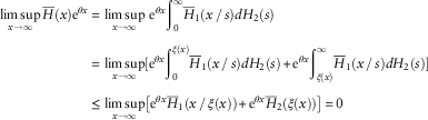 $$\eqalignno{ \mathop {{\rm lim}\,{\rm sup}}\limits_{x\to\infty} \overline{H} (x){\rm e}^{{\theta x}} \,{\equals}\, & \mathop {{\rm lim}\,{\rm sup}}\limits_{x\to\infty} \,{\rm e}^{{\theta x}} {\int}_0^\infty \overline{H} _{1} (x\,/\,s)dH_{2} (s) \cr \,{\equals}\, & \mathop {{\rm lim}\,{\rm sup}}\limits_{x\to\infty} [{\rm e}^{{\theta x}} {\int}_0^{\xi (x)} \overline{H} _{1} (x\,/\,s)dH_{2} (s){\plus}{\rm e}^{{\theta x}} {\int}_{\xi (x)}^\infty \overline{H} _{1} (x\,/\,s)dH_{2} (s)] \cr \leq & \mathop {{\rm lim}\,{\rm sup}}\limits_{x\to\infty} \left[ {{\rm e}^{{\theta x}} \overline{H} _{1} (x\,/\,\xi (x)){\plus}{\rm e}^{{\theta x}} \overline{H} _{2} (\xi (x))} \right]\,{\equals}\,0 $$
The last equality holds by the Hypothesis (3.1). Hence H is light-tailed. For the second part consider
 $$\eqalignno{ \mathop {{\rm lim}\,{\rm sup}}\limits_{x\to\infty} \overline{H} (x){\rm e}^{{\theta x}} \,{\equals}\, & \mathop {{\rm lim}\,{\rm sup}}\limits_{x\to\infty} [{\rm e}^{{\theta x}} {\int}_0^{\xi (x)} \overline{H} _{1} (x\,/\,s)dH_{2} (s){\plus}{\rm e}^{{\theta x}} {\int}_{\xi (x)}^\infty \overline{H} _{1} (x\,/\,s)dH_{2} (s)] \cr & \geq \mathop {{\rm lim}\,{\rm sup}}\limits_{x\to\infty} \left[ {{\rm e}^{{\theta x}} \overline{H} _{1} (x\,/\,\xi (x))\overline{H} _{2} (\xi (x))} \right]\,{\equals}\,\infty $$
The last equality holds by Hypothesis (3.2). Hence H is heavy-tailed.
The conditions in Theorem 3.1 can be easily verified and enables us to provide a classification of the asymptotic tail behaviour of products of random variables with more general distributions. Notice that the distributions considered in Su & Chen (Reference Su and Chen2006) correspond to distributions with log-tail probabilities decaying at a linear rate, i.e.
 $${\minus}{\rm log}\bar{{H_{1} }} (s)\,{\equals}\,O(s)$$
, while the distributions in Arendarczyk & Dębicki (Reference Arendarczyk and Dębicki2011) have log-tail probabilities decaying at a power rate, i.e.
$${\minus}{\rm log}\bar{{H_{1} }} (s)\,{\equals}\,O(s)$$
, while the distributions in Arendarczyk & Dębicki (Reference Arendarczyk and Dębicki2011) have log-tail probabilities decaying at a power rate, i.e.
 $${\minus}{\rm log}\overline{{H_{i} }} (s)\,{\equals}\,O(s^{{p_{i} }} )$$
, i=1, 2. The following example considers distributions with log-tail probabilities decaying at an exponential rate, i.e.
$${\minus}{\rm log}\overline{{H_{i} }} (s)\,{\equals}\,O(s^{{p_{i} }} )$$
, i=1, 2. The following example considers distributions with log-tail probabilities decaying at an exponential rate, i.e.
 $${\minus}{\rm log}\overline{{H_{i} }} (s)\,{\equals}\,O({\rm e}^{s} )$$
.
$${\minus}{\rm log}\overline{{H_{i} }} (s)\,{\equals}\,O({\rm e}^{s} )$$
.
Example 3.2 (Gumbellian products): Let H i (x)=1−exp{−e x +1}, x>0. We choose ξ(x)=x γ , with 0<γ<1. Then
 $$\mathop {{\rm lim}}\limits_{x\to\infty} \overline{H} (x){\rm e}^{{\theta x}} \,{\equals}\,\mathop {{\rm lim}}\limits_{x\to\infty} {\rm e}^{{\theta x{\plus}1}} \left( {{\rm exp}\left\{ {{\minus}{\rm e}^{{x^{{1\,{\minus}\,\gamma }} }} } \right\}{\plus}{\rm exp}\left\{ {{\minus}{\rm e}^{{x^{\gamma } }} } \right\}} \right)\,{\equals}\,0,\quad \forall \theta \,\gt\,0$$
Then the product of two random variables with Gumbellian-type distributions is always light-tailed. The same holds true if we replace H
2 with a Weibullian distribution with shape parameter p>1. Choose ξ(x)=x
γ
, with ![]() ≤γ<1 and observe that
≤γ<1 and observe that
 $$\mathop {{\rm lim}}\limits_{x\to\infty} \overline{H} (x){\rm e}^{{\theta x}} \,{\equals}\,\mathop {{\rm lim}}\limits_{x\to\infty} \,{\rm e}^{{\theta x}} \left( {{\rm exp}\left\{ {{\minus}{\rm e}^{{x^{{1\,{\minus}\,\gamma }} }} {\plus}1} \right\}{\plus}x^{\delta } {\rm e}^{{{\minus}x^{{\gamma p}} }} } \right)\,{\equals}\,0,\quad {\rm for}\;\theta \in(0,1)$$
3.2 Maximum domains of attraction and subexponentiality
The scenario in the Fréchet domain of attraction is well understood. Breiman’s Breiman (Reference Breiman1965) lemma implies that a PH scale mixture distribution is in the Fréchet domain of attraction if its scaling distribution is in the same domain:
Lemma 3.3
(Breiman, Reference Breiman1965): If
 $$H\in{\cal R}_{{{\minus}\alpha }} $$
and M
G
(α+ε)<∞ for some ε>0, then
$$H\in{\cal R}_{{{\minus}\alpha }} $$
and M
G
(α+ε)<∞ for some ε>0, then
 $$F\in{\cal R}_{{{\minus}\alpha }} $$
and
$$F\in{\cal R}_{{{\minus}\alpha }} $$
and
 $$\overline{F} \:(x)\,{\equals}\,M_{G} (\alpha )\overline{H} (x)(1{\plus}o(1)),\quad \quad x\to\infty$$
where M G (α) is the α-moment of G.
PH distributions are light-tailed so all their moments are finite. Therefore, a PH scale mixture distribution with a scaling distribution in the Fréchet domain of attraction remains in the same domain. Furthermore, the norming constants for a PH scale mixture distribution F can be chosen as the norming constants of H divided by the α-moment of the PH distribution G, i.e.
 $$d_{n} \,{\equals}\,0,\quad c_{n} \,{\equals}\,{1 \over {M_{G} (\alpha )}}\left( {{1 \over {\overline{H} }}} \right)^{\leftarrow} (n)$$
Moreover, when the conditions of Breiman’s lemma are satisfied, then the scaling and the PH scale mixture distributions are regularly varying with the same index of regular variation, thus implying that the tail probabilities of both distributions are asymptotically proportional (with the reciprocal of the α-moment of the PH distribution being the proportionality constant). This implies that the class of PH scale mixture distributions can provide exact asymptotic approximations of the tail probabilities of regularly varying distributions.
It is interesting to note that the converse of Breiman’s lemma does not hold true in general. Such a problem is considered to be challenging and has attracted considerable research interest, thus resulting in a rich variety of results proving sufficient conditions and counterexamples; for instance, Jessen & Mikosch (Reference Jessen and Mikosch2006) provide a comprehensive list of earlier references; the most general results are given in Jacobsen et al. (Reference Jacobsen, Mikosch and Rosinski2009) and Denisov & Zwart (Reference Denisov and Zwart2007) (see also Damen et al., Reference Damen, Mikosch, Rosinski and Samorodnitsky2014 for a multivariate version). It is not difficult to verify that some subclasses (for instance, exponential, Erlang and hyperexponential) of PH distributions satisfy the sufficient conditions for the converse of Breiman’s lemma provided in Jacobsen et al. (Reference Jacobsen, Mikosch and Rosinski2009). We also conjecture that in general PH distributions satisfy the above conditions but a proof remains unknown to us.
The situation is less understood in the Gumbel domain of attraction. We start by noting that in the Gumbel case, a PH scale mixture F and its scaling distribution H will have very different tail behaviours (this is contrast to the Fréchet case where Breiman’s lemma implies that these have asymptotically proportional tail behaviour). In particular, the tail probability of a scaling distribution in the Gumbel domain of attraction is tail equivalent to a von Mises functions, hence rapidly varying. In such a case the tail distribution of the PH scale mixture will be much heavier than its scaling distribution:
Proposition 3.4
If
 $$H\in{\cal R}_{{{\minus}\infty}} $$
, then
$$H\in{\cal R}_{{{\minus}\infty}} $$
, then
 $$\mathop {{\rm lim}\,{\rm sup}}\limits_{x\to\infty} {{\overline{H} (x)} \over {\overline{F} \:(x)}}\,{\equals}\,0$$
Proof. To show this we take t>1 and observe that there exists a constant C such that
 $$\overline{F} \:(x)\,{\equals}\,\def\Bbb{\tf="Macopen"}{\Bbb P}[SY\,\gt\,x]\geq {\Bbb P}[SY\,\gt\,x,Y\geq t]\geq {\Bbb P}[S\,\gt\,x\,/\,t]{\Bbb P}[Y\geq t]\,{\equals}\,\overline{H} (x\,/\,t)C$$
Then
 $$\mathop {{\rm lim}\,{\rm sup}}\limits_{x\to\infty} {{\overline{H} (x)} \over {\overline{F} \:(x)}}\leq {1 \over C}\,\mathop {{\rm lim}\,{\rm sup}}\limits_{x\to\infty} {{\overline{H} (x)} \over {\overline{H} (x\,/\,t)}}\,{\equals}\,0,\quad t\,\gt\,1$$
The lognormal and Weibullian distributions are rapidly varying.
Remark 3.5 This result fleshes out a limitation of the aforementioned approach for approximating distributions in the Gumbel domain of attraction. The tail probability of a PH scale mixture distribution will be much heavier than its target distribution, if the scaling distribution is chosen within the same family of target distributions and with similar parameters. We show later that in some cases we are able to construct PH scale mixture distributions with the same asymptotic behaviour as their target distributions if we vary the value of parameters. Such is the case of Weibullian distributions.
Next we look for sufficient conditions of the scaling distribution so its corresponding PH scale mixture will belong to the Gumbel domain of attraction and be subexponential. We restrict our focus to PH distributions with sub-intensity matrices having only real eigenvalues.
Theorem 3.6
Let
 $$V(x)\,{\equals}\,({\minus}1)^{{\eta {\minus}1}} {\cal L}_{{1\,/\,S}}^{{(\eta {\minus}1)}} (x)$$
where η is the largest dimension among the Jordan blocks associated to the largest eigenvalue of the sub-intensity matrix. If V(⋅) is a von Mises function, then F∈MDA(Λ). Moreover, F is subexponential if
$$V(x)\,{\equals}\,({\minus}1)^{{\eta {\minus}1}} {\cal L}_{{1\,/\,S}}^{{(\eta {\minus}1)}} (x)$$
where η is the largest dimension among the Jordan blocks associated to the largest eigenvalue of the sub-intensity matrix. If V(⋅) is a von Mises function, then F∈MDA(Λ). Moreover, F is subexponential if
 $$\mathop {{\rm lim}\,{\rm inf}}\limits_{x\to\infty} {{V(tx)V^{\prime} (x)} \over {V^{\prime} (tx)V(x)}}\,\gt\,1,\quad \quad \forall t\,\gt\,1$$
Proof. We can write that
 $$\overline{F} \:(x)\,{\equals}\,\mathop{\sum}\limits_{j\,{\equals}\,1}^m \mathop{\sum}\limits_{k\,{\equals}\,0}^{\eta _{j} {\minus}1} {\int}_0^\infty c_{{jk}} \left( {{x \over s}} \right)^{k} {\rm e}^{{{\minus}\lambda _{j} x\,/\,s}} dH(s)\,{\equals}\,\mathop{\sum}\limits_{j\,{\equals}\,1}^m \mathop{\sum}\limits_{k\,{\equals}\,0}^{\eta _{j} {\minus}1} c_{{jk}} \:{{({\minus}1)^{k} x^{k} } \over {\lambda _{j}^{k} }}\:{\cal L}_{{1\,/\,S}}^{{(k)}} (\lambda _{j} x)$$
Since
 $$V(x)\,{\equals}\,({\minus}1)^{{\eta {\minus}1}} {\cal L}_{{1\,/\,S}}^{{(\eta {\minus}1)}} (x)$$
is a von Mises function, then V(x) is of rapid variation (Bingham et al., Reference Bingham, Goldie and Teugels1987). This implies that
$$V(x)\,{\equals}\,({\minus}1)^{{\eta {\minus}1}} {\cal L}_{{1\,/\,S}}^{{(\eta {\minus}1)}} (x)$$
is a von Mises function, then V(x) is of rapid variation (Bingham et al., Reference Bingham, Goldie and Teugels1987). This implies that
 $$\overline{F} \:(x) \sim c{{x^{{\eta {\minus}1}} } \over {\lambda ^{{\eta {\minus}1}} }}V(\lambda x)$$
where c is some constant, −λ is the largest eigenvalue of the sub-intensity matrix and η the largest dimension among the Jordan blocks associated to −λ. Then it is not difficult to see that
 $$\mathop {{\rm lim}}\limits_{x\to\infty} {{\overline{F} \:(x)F^{{\prime\!\prime}} (x)} \over {(F^{\prime} (x))^{2} }}\,{\equals}\,\mathop {{\rm lim}}\limits_{x\to\infty} {{V(\lambda x)({\minus}V^{{\prime\!\prime}} (\lambda x))} \over {({\minus}V^{\prime} (\lambda x))^{2} }}\,{\equals}\,{\minus}1$$
This holds true because by hypothesis
 $$V(x)\,{\equals}\,({\minus}1)^{{\eta {\minus}1}} {\cal L}_{{1\,/\,S}}^{{(\eta {\minus}1)}} (x)$$
is a von Mises function. Hence F∈MDA(Λ) and the first part result follows. For the second part, we observe that the auxiliary function
$$V(x)\,{\equals}\,({\minus}1)^{{\eta {\minus}1}} {\cal L}_{{1\,/\,S}}^{{(\eta {\minus}1)}} (x)$$
is a von Mises function. Hence F∈MDA(Λ) and the first part result follows. For the second part, we observe that the auxiliary function
 $$a(x)\,{\equals}\,\overline{F} \:(x)\,/\,F^{\,'} (x)$$
obeys the following asymptotic equivalence:
$$a(x)\,{\equals}\,\overline{F} \:(x)\,/\,F^{\,'} (x)$$
obeys the following asymptotic equivalence:
 $$a(x)\,{\equals}\,{{\overline{F} \:(x)} \over {F^{\,'} (x)}} \sim {{V(\lambda x)} \over {{\minus}\lambda V^{\,'} (\lambda x)}}$$
The distribution F is subexponential if
 $$\mathop {{\rm lim}\,{\rm inf}}\limits_{x\to\infty} {{a(tx)} \over {a(x)}}\,{\equals}\,\mathop {{\rm lim}\,{\rm inf}}\limits_{x\to\infty} {{V(\lambda tx)V^{\prime} (\lambda x)} \over {V^{\prime} (\lambda tx)V(\lambda x)}}\,\gt\,1,\quad \quad \forall t\,\gt\,1$$
hence subexponentiality of F follows.
Theorem 3.6 can be applied to the lognormal case:
Example 3.7 (Lognormal scaling): Assume H~LN(μ, σ 2), then F is a subexponential distribution in the Gumbel domain of attraction.
Proof. W.l.o.g. we can assume μ=0 since e μ is a scaling constant. In such a case the symmetry of the normal distribution implies that the Laplace–Stieltjes transform of 1/S is the same as that of S, i.e.
 $${\cal L}_{{1\,/\,S}} (x)\,{\equals}\,{\cal L}_{S} (x)$$
An asymptotic approximation of the kth derivative of the Laplace–Stieltjes transform of the lognormal distribution is given in Asmussen et al. (Reference Asmussen, Jensen and Rojas-Nandayapa2016):
 $${\cal L}_{S}^{{(k)}} (x)\,{\equals}\,({\minus}1)^{k} {\cal L}_{S} (x){\rm exp}\left\{ {{\minus}k\omega _{0} (x){\plus}{1 \over 2}\sigma _{0} (x)^{2} k^{2} } \right\}\left( {1{\plus}o(1)} \right)$$
where
 $$\omega _{k} (x)\,{\equals}\,{\cal W}(x\sigma ^{2} {\rm e}^{{k\sigma ^{2} }} ),\quad \sigma _{k} (x)^{2} \,{\equals}\,{{\sigma ^{2} } \over {1{\plus}\omega _{k} (x)}}$$
and
 $${\cal W}( \cdot )$$
is the Lambert W function. Hence we verify that
$${\cal W}( \cdot )$$
is the Lambert W function. Hence we verify that
 $$\eqalignno{ \mathop {{\rm lim}}\limits_{x\to\infty} {{V(x)\left( {{\minus}V^{{\prime\!\prime}} (x)} \right)} \over {\left( {{\minus}V^{\prime} (x)} \right)^{2} }}\,{\equals}\, & \mathop {{\rm lim}}\limits_{x\to\infty} {{{\rm e}^{{{\minus}(\eta {\minus}1)\omega _{0} (x){\plus}{1 \over 2}\,\sigma _{0} (x)^{2} (\eta {\minus}1)^{2} }} \cdot \left( {{\minus}{\rm e}^{{{\minus}(\eta {\plus}1)\omega _{0} (x){\plus}{1 \over 2}\,\sigma _{0} (x)^{2} (\eta {\plus}1)^{2} }} } \right)} \over {{\rm e}^{{{\minus}2\eta \omega _{0} (x){\plus}\sigma _{0} (x)^{2} \eta ^{2} }} }} \cr \,{\equals}\, & {\minus}\!\mathop {{\rm lim}}\limits_{x\to\infty} \,{\rm exp}\left\{ {\sigma _{0} (x)^{2} } \right\}\,{\equals}\,{\minus}\!\mathop {{\rm lim}}\limits_{x\to\infty} \,{\rm exp}\left\{ {{{\sigma ^{2} } \over {1{\plus}\omega _{0} (x)}}} \right\} $$
As ω k (x) is asymptotically of order log(x) as x→∞, then σ 2(1+ω 0(x))−1 →0 as x→∞. Then the last limit is equal to −1, so we have shown that F(x)∈MDA(Λ). Furthermore
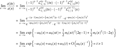 $$\eqalignno{ \mathop {{\rm lim}}\limits_{x\to\infty} {{a(tx)} \over {a(x)}}\,{\equals}\, & \mathop {{\rm lim}}\limits_{x\to\infty} {{({\minus}1)^{{\eta {\minus}1}} {\cal L}_{{1\,/\,S}}^{{(\eta {\minus}1)}} (tx) \cdot ({\minus}1)^{{\eta {\minus}1}} {\cal L}_{{1\,/\,S}}^{{(\eta )}} (x)} \over {({\minus}1)^{{\eta {\minus}1}} {\cal L}_{{1\,/\,S}}^{{(\eta )}} (tx) \cdot ({\minus}1)^{{\eta {\minus}1}} {\cal L}_{{1\,/\,S}}^{{(\eta {\minus}1)}} (x)}} \cr \,{\equals}\, & \mathop {{\rm lim}}\limits_{x\to\infty} {{{\rm e}^{{{\minus}(\eta {\minus}1)\omega _{0} (xt){\plus}{1 \over 2}\,\sigma _{0} (xt)^{2} (\eta {\minus}1)^{2} }} \cdot {\rm e}^{{{\minus}\eta \omega _{0} (x){\plus}{1 \over 2}\,\sigma _{0} (x)^{2} \eta ^{2} }} } \over {{\rm e}^{{{\minus}\eta \omega _{0} (xt){\plus}{1 \over 2}\,\sigma _{0} (xt)^{2} \eta ^{2} }} \cdot {\rm e}^{{{\minus}(\eta {\minus}1)\omega _{0} (x){\plus}{1 \over 2}\,\sigma _{0} (x)^{2} (\eta {\minus}1)^{2} }} }} \cr \,{\equals}\, & \mathop {{\rm lim}}\limits_{x\to\infty} exp\left\{ {{\minus}\omega _{0} (x){\plus}\omega _{0} (xt){\plus}{1 \over 2}\sigma _{0} (xt)^{2} (2\eta {\minus}1){\plus}{1 \over 2}\sigma _{0} (x)^{2} (1{\minus}2\eta )} \right\} \cr \,{\equals}\, & \mathop {{\rm lim}}\limits_{x\to\infty} exp\left\{ {{\minus}\omega _{0} (x){\plus}\omega _{0} (x){\plus}\omega _{0} (t){\plus}O\left( {\omega _{0} (x)^{{{\minus}1}} } \right)} \right\}\,{\equals}\,t\,\gt\,1 $$
Thus F is a subexponential distribution.
Example 3.8 (Exponential scaling): Let H~exp(β). Then F is a subexponential distribution in the Gumbel domain of attraction.
Proof. Observe that 1/S has an inverse gamma distribution with a Laplace–Stieltjes transform given in terms of a modified Bessel function of the second kind (Ragab, Reference Ragab1965):
 $${\cal L}_{{1\,/\,S}} (x)\,{\equals}\,{\int}_0^\infty{} {{\rm e}^{{{\minus}x\,/\,s}} \beta {\rm e}^{{{\minus}\beta s}} ds} \,{\equals}\,2\sqrt {\beta x} {\rm BesselK}\left( {1,2\sqrt {\beta x} } \right)$$
Furthermore, its nth derivative can be calculated explicitly also in terms of a modified Bessel function of the second kind:
 $${\cal L}_{{1\,/\,S}}^{{(n)}} (x)\,{\equals}\,{\int}_0^\infty \left( {{\minus}{1 \over s}} \right)^{n} {\rm e}^{{{\minus}x\,/\,s}} \beta {\rm e}^{{{\minus}\beta s}} ds\,{\equals}\,({\minus}1)^{n} \cdot 2\:\beta ^{{{{n{\plus}1} \over 2}}} x^{{{\minus}{{n{\minus}1} \over 2}}} {\rm Bessel}\,{\rm K}\left( {n{\minus}1,2\sqrt {\beta x} } \right)$$
Asymptotically it holds true that
 $${\cal L}_{{1\,/\,S}}^{{(n)}} (x)\!\sim\!({\minus}1)^{n} \sqrt \pi \beta ^{{{{2n{\plus}1} \over 4}}} x^{{{\minus}{{2n{\minus}1} \over 4}}} {\rm e}^{{{\minus}2\sqrt {\beta x} }} ,\quad x\to\infty$$
Hence, it follows that
 $$\mathop {{\rm lim}}\limits_{x\to\infty} {{V(x)({\minus}V^{{''}} (x))} \over {({\minus}V^{'} (x))^{2} }}\,{\equals}\,{\minus}1$$
Therefore, V(x) is a von Mises function and F∈MDA(Λ). Moreover, if t>1 then
 $$\mathop {{\rm lim}}\limits_{x\to\infty} {{a(tx)} \over {a(x)}}\,{\equals}\,\mathop {{\rm lim}}\limits_{x\to\infty} {{V(tx)V^{'} (x)} \over {V^{'} (tx)V(x)}}\,{\equals}\,\sqrt t \,\gt\,1$$
Thus F is a subexponential distribution.
Remark 3.9
Notice that it is possible to generalise the result of the previous example for a γ scaling distribution, because an expression for the Laplace–Stieltjes transform of an inverse gamma distribution is known and given in terms of a modified Bessel function of the second kind. However, it involves a number of tedious calculations and therefore omitted. Note as well that in such a case it is possible to test directly if
 $$\overline{F} \:$$
is a von Mises function, but the calculations become cumbersome. Finally, we remark that the results of Liu & Tang (Reference Liu and Tang2010) imply the subexponentiality of the exponential case.
$$\overline{F} \:$$
is a von Mises function, but the calculations become cumbersome. Finally, we remark that the results of Liu & Tang (Reference Liu and Tang2010) imply the subexponentiality of the exponential case.
Remark 3.10 If H is a discrete scaling distribution, then we can obtain an analogue result to that of Theorem 3.6. Define
 $${\cal D}{\cal L}_{{1\,/\,S}} (x)\,{\equals}\,\mathop{\sum}\limits_{i\,{\equals}\,1}^\infty {\rm e}^{{{\minus}x\,/\,i}} p(i)$$
as the Laplace–Stieltjes transform of discrete scaling random variable S with probability mass function p(i). Then the tail probability of the PH scale mixture is:
 $$\overline{F} \:(x)\,{\equals}\,\mathop{\sum}\limits_{j\,{\equals}\,1}^m \mathop{\sum}\limits_{k\,{\equals}\,0}^{\eta _{j} {\minus}1} \mathop{\sum}\limits_{i\,{\equals}\,1}^\infty c_{{jk}} \left( {{x \over i}} \right)^{k} {\rm e}^{{{\minus}\lambda _{j} x\,/\,i}} p(i)\,{\equals}\,\mathop{\sum}\limits_{j\,{\equals}\,1}^m \mathop{\sum}\limits_{k\,{\equals}\,0}^{\eta _{j} {\minus}1} c_{{jk}} \:{{({\minus}1)^{k} x^{k} } \over {\lambda _{j}^{k} }}\:{\cal D}{\cal L}_{{1\,/\,S}}^{{(k)}} (\lambda _{j} x)$$
If
 $$V(x)\,{\equals}\,({\minus}1)^{{\eta {\minus}1}} {\cal D}{\cal L}_{{1\,/\,S}}^{{(\eta {\minus}1)}} (x)$$
is a von Mises function, then F∈MDA(Λ).
$$V(x)\,{\equals}\,({\minus}1)^{{\eta {\minus}1}} {\cal D}{\cal L}_{{1\,/\,S}}^{{(\eta {\minus}1)}} (x)$$
is a von Mises function, then F∈MDA(Λ).
We close this section with an important remark regarding Weibullian scalings.
Remark 3.11 (Weibullian scaling): A non-negative distribution H is said to be Weibullian with shape parameter p>0 (Arendarczyk & Dębicki, Reference Arendarczyk and Dębicki2011) if
 $$\overline{H} (s)\,{\equals}\,Cs^{\delta } {\rm exp}({\minus}\lambda s^{p} )(1{\plus}o(1)),\quad \lambda ,C\,\gt\,0,\delta \in{\Bbb R}$$
A Weibullian distribution with parameter p is heavy-tailed if 0<p<1, while it is light-tailed if p≥1. Notice that a PH distribution is Weibullian with shape parameter equal to 1. Therefore, lemma 2.1 of Arendarczyk & Dębicki (Reference Arendarczyk and Dębicki2011) implies that a PH scale mixture having a Weibullian scaling distribution with scale parameter p will be Weibullian with shape parameter p 1(1+p 1)−1<1, thus heavy-tailed. Furthermore, lemma 2.1 in Arendarczyk & Dębicki (Reference Arendarczyk and Dębicki2011) provides exact expressions for each of the parameters C, δ and λ, so in principle one can use this result to replicate exactly the tail behaviour of a Weibullian distribution via a PH scale mixture distribution.
4 Discrete Scaling Distributions
Next we focus on the case of PH scale mixture distributions having scaling distributions supported over countable sets of strictly positive numbers. These distributions are particularly tractable since these correspond to distributions of absorption times of Markov jump processes with an infinite number of transient states. This class of distributions is of great importance for applications involving heavy-tailed phenomena, since a variety of quantities of interest can be calculated exactly. Such is the case of ruin probabilities in the Crámer–Lundberg process having claims sizes distributed according to a PH scale mixture (cf. Bladt et al., Reference Bladt, Campillo Navarro and Nielsen2015a, Reference Bladt, Nielsen and Samorodnitsky2015b; Peralta et al.,Reference Peralta, Rojas-Nandayapa, Xie and Yao2016). Notice for instance, that such exact results are not available for the case of continuous scaling distributions.
We remark, however, that some of the methodologies for determining domains of attraction and subexponentiality described in the previous section are not always implementable in a straightforward way for discrete scaling distributions. One of the main difficulties is the calculation of asymptotic equivalent expressions for the infinite series defining the tail probabilities. Below we describe a simple methodology which can be used to extend results for continuous scaling distributions to their discrete scaling distributions counterparts; such a methodology provides mild conditions under which the asymptotical behaviour of an infinite series is asymptotically equivalent to that of a certain function defined via a definite integral.
Proposition 4.1
Let
 $$I_{u} \,\colon\,{\bf Z}^{{\plus}} \!\!\!\to\!\def\Bbb{\tf="Macopen"}{\Bbb R}^{{\plus}} $$
be collection of functions indexed by u∈(0, ∞). Suppose that for each u>0 there exists a measurable and bounded function
$$I_{u} \,\colon\,{\bf Z}^{{\plus}} \!\!\!\to\!\def\Bbb{\tf="Macopen"}{\Bbb R}^{{\plus}} $$
be collection of functions indexed by u∈(0, ∞). Suppose that for each u>0 there exists a measurable and bounded function
 $$I{\prime}_{u} \,\colon\,\def\Bbb{\tf="Macopen"}{\Bbb R}^{{\plus}}\!\!\to{\Bbb R}$$
such that I(u; k)=I′(u; k) for all
$$I{\prime}_{u} \,\colon\,\def\Bbb{\tf="Macopen"}{\Bbb R}^{{\plus}}\!\!\to{\Bbb R}$$
such that I(u; k)=I′(u; k) for all
 $$k\in\def\Bbb{\tf="Macopen"}{\Bbb Z}^{{\plus}} $$
and
$$k\in\def\Bbb{\tf="Macopen"}{\Bbb Z}^{{\plus}} $$
and
 $${\int}_0^\infty I'(u;\,y)dy\,{\minus}\,M(u)\leq \mathop{\sum}\limits_{k\,{\equals}\,0}^\infty I(u;\,k)\leq {\int}_0^\infty I{\prime}(u;\,y)dy{\plus}M(u)$$
where M(u)≥max{I′(u; y):y>0} is some upper bound for the function I′(u;y). If
 $$\mathop {{\rm lim}}\limits_{u\to\infty} {{M(u)} \over {{\int}_0^\infty I{\prime}(u;\,y)dy}}\,{\equals}\,0$$
then the following asymptotic relationship holds
 $$\mathop {{\rm lim}}\limits_{u\to\infty} {{\mathop{\sum}\limits_{k\,{\equals}\,0}^\infty I(u;\,k)} \over {{\int}_0^\infty I{\prime}(u;\,y)dy}}\,{\equals}\,1$$
The method provides a verifiable condition under which the infinite series can be replaced by an asymptotic integral. The next example is taken from Bladt et al. (Reference Bladt, Campillo Navarro and Nielsen2015a, Reference Bladt, Nielsen and Samorodnitsky2015b).
Example 4.2
(Zeta scaling): Let α≥2 and assume H~Zeta(α). Such a distribution is determined by p(i)=i
−α
/ζ(α),
 $$i\in\def\Bbb{\tf="Macopen"}{\Bbb N}$$
and ζ(⋅) is the Riemann zeta function. Then F is in the Fréchet domain of attraction.
$$i\in\def\Bbb{\tf="Macopen"}{\Bbb N}$$
and ζ(⋅) is the Riemann zeta function. Then F is in the Fréchet domain of attraction.
We remark that Breiman’s lemma could have been used instead to determine the exact asymptotic behaviour because the tail probability
 $$\overline{H} (i)$$
, i=1, 2, … forms a regularly varying sequence, so
$$\overline{H} (i)$$
, i=1, 2, … forms a regularly varying sequence, so
 $$\overline{H} \in{\cal R}_{{{\minus}\alpha }} $$
(Bingham et al., Reference Bingham, Goldie and Teugels1987). Nevertheless, this example is included here to illustrate the simplicity of the method proposed.
$$\overline{H} \in{\cal R}_{{{\minus}\alpha }} $$
(Bingham et al., Reference Bingham, Goldie and Teugels1987). Nevertheless, this example is included here to illustrate the simplicity of the method proposed.
Proof. H is supported over all the natural numbers, so the tail probability of corresponding PH scale mixture can be written as
 $$\overline{F} \:(x)\,{\equals}\,\mathop{\sum}\limits_{i\,{\equals}\,1}^\infty p(i)\overline{G} \:(x/i)$$
Recall that the expression of
 $$\overline{G} \:( \cdot )$$
has been given in (2.1), then we have
$$\overline{G} \:( \cdot )$$
has been given in (2.1), then we have
 $$\overline{F} \:(x)\,{\equals}\,\mathop{\sum}\limits_{i\,{\equals}\,1}^\infty \mathop{\sum}\limits_{j\,{\equals}\,1}^m \mathop{\sum}\limits_{k\,{\equals}\,0}^{\eta _{j} {\minus}1} c_{{jk}} \left( {{x \over i}} \right)^{k} {\rm e}^{{{\minus}\lambda _{j} x\,/\,i}} {{i^{{{\minus}\alpha }} } \over {\zeta (\alpha )}}\,{\equals}\,\mathop{\sum}\limits_{j\,{\equals}\,1}^m \mathop{\sum}\limits_{k\,{\equals}\,0}^{\eta _{j} {\minus}1} \mathop{\sum}\limits_{i\,{\equals}\,1}^\infty {{c_{{jk}} x^{k} } \over {\zeta (\alpha )}}i^{{{\minus}(\alpha {\plus}k)}} {\rm e}^{{{\minus}\lambda _{j} x\,/\,i}} $$
Consider the functions
 $$I{\prime}_{{jk}} (x;\,y)\,{\equals}\,x^{k} y^{{{\minus}(\alpha {\plus}k)}} {\rm e}^{{{\minus}\lambda _{j} x\,/\,y}} $$
and note that each of these functions attains their single local maximum at
$$I{\prime}_{{jk}} (x;\,y)\,{\equals}\,x^{k} y^{{{\minus}(\alpha {\plus}k)}} {\rm e}^{{{\minus}\lambda _{j} x\,/\,y}} $$
and note that each of these functions attains their single local maximum at
 $$\hat{y}\,{\equals}\,\lambda _{j} x(\alpha {\plus}k)^{{{\minus}1}} \,\gt\,0$$
, for all x>0. Therefore:
$$\hat{y}\,{\equals}\,\lambda _{j} x(\alpha {\plus}k)^{{{\minus}1}} \,\gt\,0$$
, for all x>0. Therefore:
 $${\int}_0^\infty I{\prime}_{{jk}} (x;\,y)dy\,{\minus}\,M_{{jk}} (x;\,\hat{y})\leq \mathop{\sum}\limits_{i\,{\equals}\,1}^\infty x^{k} i^{{{\minus}(\alpha {\plus}k)}} {\rm e}^{{{\minus}\lambda _{j} x\,/\,i}} \leq {\int}_0^\infty I{\prime}_{{jk}} (x;\,y)dy{\plus}M_{{jk}} (x;\,\hat{y})$$
Observe that
 $$M_{{jk}} (x;\,\hat{y})\,{\equals}\,x^{k} {\rm e}^{{{\minus}(\alpha {\plus}k)}} \left( {{{\lambda _{j} } \over {\alpha {\plus}k}}} \right)^{{{\minus}(\alpha {\plus}k)}} x^{{{\minus}(\alpha {\plus}k)}} \,{\equals}\,cx^{{{\minus}\alpha }} $$
and
 $$I{\prime}_{{jk}} (x)\,\colon{\equals}\,x^{k} {\int}_0^\infty y^{{{\minus}(\alpha {\plus}k)}} {\rm e}^{{{\minus}\lambda _{j} x\,/\,y}} dy\,{\equals}\,{{\Gamma (\alpha {\plus}k{\minus}1)} \over {\lambda ^{{\alpha {\plus}k{\minus}1}} }}x^{{{\minus}\alpha {\plus}1}} $$
so
 $$M_{{jk}} (x;\,\hat{y})$$
is of negligible order with respect to I′
jk
(x). Then it follows that
$$M_{{jk}} (x;\,\hat{y})$$
is of negligible order with respect to I′
jk
(x). Then it follows that
 $$\overline{F} \:(x)\!\sim\!\mathop{\sum}\limits_{j\,{\equals}\,1}^m {\mathop{\sum}\limits_{k\,{\equals}\,0}^{\eta _{j} {\minus}1} {{{c_{{jk}} } \over {\zeta (\alpha )}}I'_{{jk}} (x)} } \,{\equals}\,\mathop{\sum}\limits_{j\,{\equals}\,1}^m {\mathop{\sum}\limits_{k\,{\equals}\,0}^{\eta _{j} {\minus}1} {{{c_{{jk}} \Gamma (\alpha {\plus}k{\minus}1)} \over {\zeta (\alpha )\lambda ^{{\alpha {\plus}k{\minus}1}} }}x^{{{\minus}\alpha {\plus}1}} } } ,\quad x\to\infty$$
Thus F(x)∈MDA(Φ
α−1). Let
 $$C\,{\equals}\,\mathop{\sum}\limits_{j\,{\equals}\,1}^m \mathop{\sum}\limits_{k\,{\equals}\,0}^{\eta _{j} {\minus}1} {{c_{{jk}} \Gamma (\alpha {\plus}k{\minus}1)} \over {\zeta (\alpha )\lambda ^{{\alpha {\plus}k{\minus}1}} }}$$
, then the norming constants can be chosen as
$$C\,{\equals}\,\mathop{\sum}\limits_{j\,{\equals}\,1}^m \mathop{\sum}\limits_{k\,{\equals}\,0}^{\eta _{j} {\minus}1} {{c_{{jk}} \Gamma (\alpha {\plus}k{\minus}1)} \over {\zeta (\alpha )\lambda ^{{\alpha {\plus}k{\minus}1}} }}$$
, then the norming constants can be chosen as
 $$d_{n} \,{\equals}\,0,\quad c_{n} \,{\equals}\,\left( {{1 \over {\overline{F} \:}}} \right)^{\leftarrow} (n)\,{\equals}\,\left( {{C \over n}} \right)^{{{1 \over {\alpha {\minus}1}}}} $$
Example 4.3 (Geometric scaling): Let H~Geo(p) and G be PH distribution whose sub-intensity matrix has only real eigenvalues. Then F is a subexponential distribution in the Gumbel domain of attraction.
Proof. Let p(i)=pq i where q=1−p. Since the geometric distribution has unbounded support, then the associated PH scale mixture is heavy-tailed. We next verify that it belongs to the Gumbel domain of attraction.
 $$\overline{F} \:(x)\,{\equals}\,\mathop{\sum}\limits_{i\,{\equals}\,1}^\infty \overline{G} \:\left( {x\,/\,i} \right)pq^{i} $$
Let
 $$I{\prime}(x;y)\,{\equals}\,\overline{G} \:(x/y)p{\rm exp}\left\{ {{\minus}\!\mid\!{\rm log}q\!\mid\!y} \right\}$$
satisfies the conditions in Proposition 4.1. Since the sine and cosine functions are bounded, then it is not difficult to use Proposition 2.1 to show that there exists a constant c
1 such that
$$I{\prime}(x;y)\,{\equals}\,\overline{G} \:(x/y)p{\rm exp}\left\{ {{\minus}\!\mid\!{\rm log}q\!\mid\!y} \right\}$$
satisfies the conditions in Proposition 4.1. Since the sine and cosine functions are bounded, then it is not difficult to use Proposition 2.1 to show that there exists a constant c
1 such that
 $$M(x)\,\colon\!{\equals}\,I(x;\hat{y})\leq x^{{{k \over 2}}} {\rm e}^{{{\minus}2\sqrt {x\lambda \,\mid\,{\rm log}\,q\,\mid\,} }} (c_{1} {\plus}o(1)),\quad \quad x\to\infty$$
where λ is the largest eigenvalue in absolute value and k its largest multiplicity. If the sub-intensity matrix has real eigenvalues then by using lemma 2.1 in Arendarczyk & Dębicki (Reference Arendarczyk and Dębicki2011) we obtain that
 $${\int}_0^\infty I{\prime}(x;y)dy\,{\equals}\,p{\int}_0^\infty \overline{G} \:(x/y){\rm e}^{{{\minus}y\,\mid\,{\rm log}\,q\,\mid\,}} dy\,{\equals}\,x^{{k\,/\,2{\plus}1\,/\,4}} {\rm e}^{{{\minus}2\sqrt {x\lambda \,\mid\,{\rm log}\,q\,\mid\,} }} (C_{1} {\plus}o(1)),\quad \quad x\to\infty$$
So, the value of M(x) is asymptotically negligible with respect to the value of the integral and we conclude that
 $$\overline{F} \:(x)\,\sim\,p{\int}_0^\infty {\overline{G} \:\left( {x\,/\,y} \right){\rm e}^{{{\minus}y\,\mid\,{\rm log}\,q\,\mid\,}} dy} \,{\equals}\,{p \over {\,\mid\!{\rm log}\,q\!\mid\,}}{\int}_0^\infty {\overline{G} \:\left( {x\,/\,y} \right)dH(y)} $$
where H~exp(|logq|). Hence, by tail equivalence, the distribution F inherits all the asymptotic properties of its continuous counterpart, namely, a PH scale distribution with exponential scaling distribution with parameter |logq|.
Remark 4.4
We shall recall that the geometric version can be seen as the discrete counterpart of the exponential distribution obtained as a discretisation. More precisely, the geometric distribution can be seen as a distribution supported over
 $$\def\Bbb{\tf="Macopen"}{\Bbb Z}^{{\plus}} $$
and defined by
$$\def\Bbb{\tf="Macopen"}{\Bbb Z}^{{\plus}} $$
and defined by
 $$H(k)\,{\equals}\,{\cal H}(k),\quad k\,{\equals}\,0,1,2, \cdots $$
where
 $${\cal H}\!\sim\!\:{\rm exp}\left( {\mid\!\!{\rm log}\,q\!\mid} \right)$$
. The probability mass function of H is given by
$${\cal H}\!\sim\!\:{\rm exp}\left( {\mid\!\!{\rm log}\,q\!\mid} \right)$$
. The probability mass function of H is given by
 $$h(k)\,{\equals}\,{\cal H}(k){\minus}{\cal H}(k{\minus}1)$$
.
$$h(k)\,{\equals}\,{\cal H}(k){\minus}{\cal H}(k{\minus}1)$$
.
This idea can be extended in order to select scaling distributions for approximating heavy-tailed distributions in the Gumbel domain of attraction. Suppose we want to approximate the tail probability of an absolutely continuous distribution
 $${\cal H}$$
supported over (0, ∞) via a discrete PH scale mixture distribution. One way to proceed is to construct a discrete distribution supported over
$${\cal H}$$
supported over (0, ∞) via a discrete PH scale mixture distribution. One way to proceed is to construct a discrete distribution supported over
 $${\cal H}$$
defined by
$${\cal H}$$
defined by
 $$h(k)\,{\equals}\,{\cal H}(k){\minus}{\cal H}(k{\minus}1)$$
; we refer to this construction as a discretisation of
$$h(k)\,{\equals}\,{\cal H}(k){\minus}{\cal H}(k{\minus}1)$$
; we refer to this construction as a discretisation of
 $${\cal H}$$
. Moreover, the density of
$${\cal H}$$
. Moreover, the density of
 $${\cal H}$$
can be used to construct a function I′(u; k). In such a case the tail behaviour of a PH scale mixture having a discretised scaling distribution inherits the asymptotic properties of its continuous counterpart.
$${\cal H}$$
can be used to construct a function I′(u; k). In such a case the tail behaviour of a PH scale mixture having a discretised scaling distribution inherits the asymptotic properties of its continuous counterpart.
This idea is better illustrated with the following example, which suggests a methodology for approximating the tail probability of a lognormal distribution.
Example 4.5
(Lognormal discretisation): Let H be a discrete lognormal distribution with parameters μ, σ and supported over {0, 1, 2, …}. Assume μ=0. The tail probability
 $$\overline{F} \:$$
is given by
$$\overline{F} \:$$
is given by
 $$\overline{F} \:(x)\,{\equals}\,\mathop{\sum}\limits_{i\,{\equals}\,1}^\infty \overline{G} \:(x\,/\,i)\left[ {H(i){\minus}H(i{\minus}1)} \right]\,{\equals}\,\mathop{\sum}\limits_{i\,{\equals}\,1}^\infty \overline{G} \:(x\,/\,i){\int}_{i{\minus}1}^i h(y)dy$$
where h(⋅) is the density of lognormal distribution. Since
 $$\overline{G} \:(x\,/\,y)$$
is increasing in y, then we can easily find a lower bound:
$$\overline{G} \:(x\,/\,y)$$
is increasing in y, then we can easily find a lower bound:
 $$\overline{F} \:(x)\,{\equals}\,\mathop{\sum}\limits_{i\,{\equals}\,1}^\infty {\int}_{i{\minus}1}^i \overline{G} \:(x\,/\,i)h(y)dy\geq {\int}_0^\infty \overline{G} \:(x\,/\,y)h(y)dy$$
For the upper bound, we have
 $$\eqalignno{ \overline{F} \:(x)\leq & \mathop{\sum}\limits_{i\,{\equals}\,1}^\infty {\int}_{i{\minus}1}^i \overline{G} \left( {{x \mathord{\left/ {\vphantom {x {(y{\plus}1)}}} \right. \kern-\nulldelimiterspace} {(y{\plus}1)}}} \right)h(y)dy\,{\equals}\,\mathop{\sum}\limits_{i\,{\equals}\,1}^\infty {\int}_{i{\minus}1}^i \overline{G} \:\left( {{x \mathord{\left/ {\vphantom {x {(y{\plus}1)}}} \right. \kern-\nulldelimiterspace} {(y{\plus}1)}}} \right)[h(y){\minus}h(y{\plus}1){\plus}h(y{\plus}1)]dy \cr \leq & {\int}_0^\infty \overline{G} \:\left( {{x \mathord{\left/ {\vphantom {x y}} \right. \kern-\nulldelimiterspace} y}} \right)h(y)dy{\plus}{\int}_0^\infty \overline{G} \:\left( {{x \mathord{\left/ {\vphantom {x {(y{\plus}1)}}} \right. \kern-\nulldelimiterspace} {(y{\plus}1)}}} \right)\left[ {h(y){\minus}h(y{\plus}1)} \right]dy $$
For the second integral in the above, we have
 $$\eqalignno{ & {\int}_0^\infty \overline{G} \left( {x/(y{\plus}1)} \right)\left[ {h(y)\,{\minus}\,h(y{\plus}1)} \right]dy \cr & \,{\equals}\,{\int}_0^1 \overline{G} \:\left( {x/(y{\plus}1)} \right)\left[ {h(y)\,{\minus}\,h(y{\plus}1)} \right]dy{\plus}{\int}_1^\infty {\overline{G} \left( {x/(y{\plus}1)} \right)\left[ {h(y){\minus}h(y{\plus}1)} \right]dy} \cr & \leq c_{1} \overline{G} \:(x/2){\plus}c_{2} {\int}_1^\infty {\overline{G} \:\left( {x\,/\,(y{\plus}1)} \right){{h(y{\plus}1)} \over {(y{\plus}1)^{\beta } }}dy} $$
where c 1, c 2>0 are some constants and 0<β<1.
It is not difficult to obtain this upper bound: first, it is easy to prove for y≥1, log(y+1)−log(y)≤1/y, consequently,
 $${{\rm log}}^2 (y{\plus}1){\minus}{{\rm log}}^2 (y)\leq 2{\rm log}(y{\plus}1)\,/\,y$$
; then we have
$${{\rm log}}^2 (y{\plus}1){\minus}{{\rm log}}^2 (y)\leq 2{\rm log}(y{\plus}1)\,/\,y$$
; then we have
 $$\eqalignno{ {{h(y)} \over {h(y{\plus}1)}}{\minus}1\,{\equals}\, & {{y{\plus}1} \over y}{\rm exp}\left\{ {{{{{\rm log}}^2 (y{\plus}1){\minus}{{\rm log}}^2 (y)} \over {2\sigma ^{2} }}} \right\}{\minus}1 \cr \leq & {\rm exp}\left\{ {{1 \over y}{\plus}{{{\rm log}(y{\plus}1)} \over {\sigma ^{2} y}}} \right\}{\minus}1 \cr \leq & c\left( {{1 \over y}{\plus}{{{\rm log}(y{\plus}1)} \over {\sigma ^{2} y}}} \right),\,{\rm where}\;c\,\gt\,0\;{\rm is}\,{\rm some}\,{\rm constant}, \cr \leq & {{c_{2} } \over {(y{\plus}1)^{\beta } }} $$
Define
 $$I{\prime}_{{jk}} (x)\,\colon\!{\equals}\,x^{k} {\int}_0^\infty y^{{{\minus}k}} {\rm e}^{{{\minus}\lambda _{j} x\,/\,y}} h(y)dy$$
From Example 3.7, we know that
 $$\eqalignno{ {\int}_0^\infty \overline{G} \left( {x\,/\,y} \right)h(y)dy\,{\equals}\, & \mathop{\sum}\limits_{j\,{\equals}\,1}^m \mathop{\sum}\limits_{k\,{\equals}\,0}^{\eta _{j} {\minus}1} c_{{jk}} {\int}_0^\infty \left( {{x \mathord{\left/ {\vphantom {x y}} \right. \kern-\nulldelimiterspace} y}} \right)^{k} {\rm e}^{{{\minus}\lambda _{j} x\,/\,y}} h(y)dy\,{\equals}\,\mathop{\sum}\limits_{j\,{\equals}\,1}^m \mathop{\sum}\limits_{k\,{\equals}\,0}^{\eta _{j} {\minus}1} c_{{jk}} {{({\minus}1)^{k} x^{k} } \over {\lambda _{j}^{k} }}{\cal L}_{Y}^{{(k)}} \left( {\lambda _{j} x} \right) \cr \,{\equals}\, & \mathop{\sum}\limits_{j\,{\equals}\,1}^m \mathop{\sum}\limits_{k\,{\equals}\,0}^{\eta _{j} {\minus}1} c_{{jk}} \:{{x^{k} } \over {\lambda _{j}^{k} }}{\cal L}_{Y} \,{\rm exp}\,\left\{ {{\minus}k\omega _{0} (\lambda _{j} x){\plus}{1 \over 2}\sigma _{0} (\lambda _{j} x)^{2} k^{2} } \right\} $$
So
 $$I{\prime}_{{jk}} (x)\,{\equals}\,\left( {{x \over {\lambda _{j} }}} \right)^{k} {\cal L}_{Y} \,{\rm exp}\,\left\{ {{\minus}k\omega _{0} \left( {\lambda _{j} x} \right){\plus}{1 \over 2}\sigma _{0} \left( {\lambda _{j} x} \right)^{2} k^{2} } \right\}$$
It is obvious that
 $$c_{1} \overline{G} \:(x\,/\,2)$$
vanishes faster than I′
jk
(x), so we can define
$$c_{1} \overline{G} \:(x\,/\,2)$$
vanishes faster than I′
jk
(x), so we can define
 $$M_{{jk}} (x)\,\colon\!{\equals}\,x^{k} {\int}_0^\infty y^{{{\minus}k{\minus}\beta }} {\rm e}^{{{\minus}\lambda _{j} x\,/\,y}} h(y)dy$$
since
 $$\eqalignno{ & c_{2} {\int}_1^\infty \overline{G} \left( {{x \mathord{\left/ {\vphantom {x {(y{\plus}1)}}} \right. \kern-\nulldelimiterspace} {(y{\plus}1)}}} \right){{h(y{\plus}1)} \over {(y{\plus}1)^{\beta } }}dy\,{\equals}\,c_{2} {\int}_2^\infty \overline{G} \left( {x/y} \right){{h(y)} \over {y^{\beta } }}dy \cr & \leq \mathop{\sum}\limits_{j\,{\equals}\,1}^m \mathop{\sum}\limits_{k\,{\equals}\,0}^{\eta _{j} {\minus}1} c_{{jk}} {\int}_0^\infty \left( {x/y} \right)^{k} y^{{{\minus}\beta }} {\rm e}^{{{\minus}\lambda _{j} x\,/\,y}} h(y)dy $$
By a similar approximation as in Example 3.7, we can see
 $$\eqalignno{ M_{{jk}} (x)\,{\equals}\, & ({\minus}1)^{{k{\plus}\beta }} {{x^{k} } \over {\lambda _{j}^{{k{\plus}\beta }} }}{\cal L}_{Y}^{{(k{\plus}\beta )}} \left( {\lambda _{j} x} \right) \cr \,{\equals}\, & {{x^{k} } \over {\lambda _{j}^{{k{\plus}\beta }} }}{\cal L}_{Y} {\rm exp}\left\{ {{\minus}\left( {k{\plus}\beta } \right)\omega _{0} \left( {\lambda _{j} x} \right){\plus}{1 \over 2}\sigma _{0} \left( {\lambda _{j} x} \right)^{2} \left( {k{\plus}\beta } \right)^{2} } \right\} $$
So M jk (x) is negligible compared to integral I′ jk (x). Thus, the PH scale mixture distribution with discrete lognormal scaling has the same asymptotic behaviour as the PH scale mixture distribution with lognormal scaling.
4.1 Non-lattice supports
The examples in the previous subsection may suggest that a PH scale mixture having a discretised scaling distribution will inherit the asymptotic properties of its continuous counterpart. However, such a discretisation cannot be made arbitrarily. The following example illustrates this fact.
Example 4.6
Let
 $$H\in{\cal R}_{{{\minus}\alpha }} $$
be a continuous distribution and S be a discrete random variable supported over {s
1, s
2, … } satisfying
$$H\in{\cal R}_{{{\minus}\alpha }} $$
be a continuous distribution and S be a discrete random variable supported over {s
1, s
2, … } satisfying
 $$\def\Bbb{\tf="Macopen"}{\Bbb P}(S\,{\equals}\,s_{i} )\,{\equals}\,H(s_{i} )\,{\minus}\, {H}(s_{{i{\minus}1}} ),\quad i\,{\equals}\,1,2, \cdots $$
Suppose there exists ![]() >0 and
>0 and
 $$i_{0} \in\def\Bbb{\tf="Macopen"}{\Bbb N}$$
such that ∀i>i
0, it holds that s
i+1>s
i
(1+
$$i_{0} \in\def\Bbb{\tf="Macopen"}{\Bbb N}$$
such that ∀i>i
0, it holds that s
i+1>s
i
(1+ ![]() ). Then
). Then
 $$\mathop {{\rm lim}\,{\rm sup}}\limits_{x\to\infty} \def\Bbb{\tf="Macopen"}{{{\Bbb P}[S\,\gt\,(1{\plus}{\epsilon})x]} \over {{\Bbb P}[S\,\gt\,x]}}\,{\equals}\,\mathop {{\rm lim}\,{\rm sup}}\limits_{i\to\infty} {{{\Bbb P}[S\,\gt\,(1{\plus}{\epsilon})s_{i} ]} \over {{\Bbb P}[S\,\gt\,s_{i} ]}}\,{\equals}\,\mathop {{\rm lim}\,{\rm sup}}\limits_{i\to\infty} {{{\Bbb P}[S\,\gt\,s_{i} ]} \over {{\Bbb P}[S\,\gt\,s_{i} ]}}\,{\equals}\,1$$
Then S does not have a regularly varying distribution. Suppose that Y~Erlang(λ, k). According to example 4.4 in Jacobsen et al. (Reference Jacobsen, Mikosch and Rosinski2009), the distribution of PH scale mixture random variable S⋅Y is not regularly varying.
Nevertheless, such a discretisation will provide a reasonable approximation to a regularly varying distribution. The following is a continuation of our previous example and it shows that such a distribution satisfies an analogue of Breiman’s lemma.
Example 4.7
Let K>0 and define H
K
a discrete distribution supported over
 $$\left\{ {s_{i} \,\colon\,i\in\def\Bbb{\tf="Macopen"}{\Bbb Z}^{{\plus}} } \right\}$$
, where s
i
=exp(i/K), and determined by
$$\left\{ {s_{i} \,\colon\,i\in\def\Bbb{\tf="Macopen"}{\Bbb Z}^{{\plus}} } \right\}$$
, where s
i
=exp(i/K), and determined by
 $$\hskip 11pcH_{K} (s_{i} )\,{\equals}\,1{\minus}s_{i}^{{{\minus}\alpha }} ,\quad \quad \forall i\in\def\Bbb{\tf="Macopen"}{\Bbb Z}^{{\plus}} $$
The distribution H
K
can be seen as a discretisation over a geometric progression of a Pareto distribution having tail probability H(x)=x
−α
supported over [1, ∞). The following argument shows that H
K
is no longer a regularly varying distribution. Notice that for all t>1 there exist
 $$n\in\def\Bbb{\tf="Macopen"}{\Bbb Z}^{{\plus}} $$
such that s
n
<t≤s
n+1, hence
$$n\in\def\Bbb{\tf="Macopen"}{\Bbb Z}^{{\plus}} $$
such that s
n
<t≤s
n+1, hence
 $$\matrix{ {\mathop {{\rm lim}\,{\rm inf}}\limits_{x\to\infty} {{\overline{H} _{K} (xt)} \over {\overline{H} _{K} (x)}}\,{\equals}\,s_{{n{\plus}1}}^{{{\minus}\alpha }} ,} & {\mathop {{\rm lim}\,{\rm sup}}\limits_{x\to\infty} {{\overline{H} _{K} (xt)} \over {\overline{H} _{K} (x)}}\,{\equals}\,\bigg\{ {\matrix{ {s_{n}^{{{\minus}\alpha }} } & {t\,\lt\,s_{{n{\plus}1}} } \cr {s_{{n{\plus}1}}^{{{\minus}\alpha }} } & {t\,{\equals}\,s_{{n{\plus}1}} } \cr } } .} \cr } $$
Thus, according to example 4.4 in Jacobsen et al. (Reference Jacobsen, Mikosch and Rosinski2009), the Mellin–Stieltjes convolution of an Erlang distribution G with the distribution H given above is no longer of regular variation (the conditions described in Proposition 4.1 are not satisfied for this example either). In spite of this, we can still analyse certain aspects of the asymptotic behaviour of such a Mellin–Stieltjes convolution. For that purpose, note that the following inequalities hold for all w>1
 $${\rm e}^{{{\minus}\alpha \,/\,K}} \overline{H} (w)\,\lt\,\overline{H} _{K} (w)\leq \overline{H} (w)$$
hence we obtain that
 $${\rm e}^{{{\minus}\alpha \,/\,K}} {\int}_0^\infty \overline{H} (x\,/\,s)dG(s)\,\lt\,{\int}_0^\infty \overline{H} _{K} (x\,/\,s)dG(s)\leq {\int}_0^\infty \overline{H} (x\,/\,s)dG(s)$$
Using Breiman’s lemma we find that
 $${\rm e}^{{{\minus}\alpha \,/\,K}} \,\lt\,{\rm lim}\,{\rm inf}{{\overline{F} \:(x)} \over {M_{G} (\alpha )\overline{H} (x)}}\leq {\rm lim}\,{\rm sup}{{\overline{F} \:(x)} \over {M_{G} (\alpha )\overline{H} (x)}}\leq 1$$
A heuristic interpretation of the inequalities above is that aysmptotically the tail probability
 $$\overline{F} \:$$
oscillates between two regularly varying tails, so this example illustrates a behaviour similar to that described by Breiman’s lemma. Notice that the range of oscillation collapses as K→∞, which is consistent with the fact that H
K
→ H weakly. A better asymptotic approximation in the following argument is particularly sharp for numerical purposes. Consider
$$\overline{F} \:$$
oscillates between two regularly varying tails, so this example illustrates a behaviour similar to that described by Breiman’s lemma. Notice that the range of oscillation collapses as K→∞, which is consistent with the fact that H
K
→ H weakly. A better asymptotic approximation in the following argument is particularly sharp for numerical purposes. Consider
 $$\overline{F} \:(x)\,{\equals}\,{\int}_0^\infty \overline{G} \:\left( {x\,/\,s} \right)dH_{K} (s)\,{\equals}\,(1{\minus}{\rm e}^{{{\minus}\alpha \,/\,K}} )\mathop{\sum}\limits_{i\,{\equals}\,0}^\infty \overline{G} \:(x{\rm e}^{{{\minus}i\,/\,K}} ){\rm e}^{{{\minus}\alpha i\,/\,K}} $$
Let
 $$I(x;i)\,{\equals}\,\overline{G} \:(x{\rm e}^{{{\minus}i\,/\,K}} ){\rm e}^{{{\minus}\alpha i\,/\,K}} $$
. The infinite series can be approximated via the integral
$$I(x;i)\,{\equals}\,\overline{G} \:(x{\rm e}^{{{\minus}i\,/\,K}} ){\rm e}^{{{\minus}\alpha i\,/\,K}} $$
. The infinite series can be approximated via the integral
 $${\int}_0^\infty I(x;y)dy\,{\equals}\,{\int}_0^\infty \overline{G} \:\left( {x{\rm e}^{{{\minus}y\,/\,K}} } \right){\rm e}^{{{\minus}\alpha y\,/\,K}} dy\,{\equals}\,K{\int}_1^\infty \overline{G} \:\left( {{x \over w}} \right)w^{{{\minus}(\alpha {\plus}1)}} dw\,{\equals}\,{K \over \alpha }{\int}_1^\infty \overline{G} \:\left( {{x \over w}} \right)dH(w)$$
Since G is such that M G (α+ε)<∞ for all ε>0, then Breiman’s lemma implies that
 $$\overline{F} \:(x)\approx\,{{1{\minus}{\rm e}^{{{\minus}\alpha \,/\,K}} } \over {\alpha \,/\,K}}M_{G} (\alpha )\overline{H} (x)$$
This approximation is consistent with the bounds found above, since for all w>0 it holds that
 $${\rm e}^{{{\minus}w}} \leq {{1{\minus}{\rm e}^{{{\minus}w}} } \over w}\leq 1$$
Hence, the asymptotic approximation suggested is contained in between the asymptotic bounds previously found.
The previous example demonstrates that the tail behaviour of a PH scale mixture distribution having a discretised scaling distribution is clearly affected by the selection of the support. Naturally, better approximations will be obtained by taking a finer partition of the support.
The natural choice is to use a discretisation of the target distribution over some lattice. However, this approach is not always suitable for numerical purposes, because in practice there is only a finite number of terms of the infinite series that can be computed, so these series are typically truncated. By selecting a discretisation over a geometric progression, we will obtain infinite series that converge at faster rates, so these can be truncated earlier. More importantly, such geometric progressions still provide reasonable approximations of the tail probability as shown above. This approach has been tested successfully in Peralta et al. (Reference Peralta, Rojas-Nandayapa, Xie and Yao2016), where they considered discretising a Pareto distribution over a geometric progression and used the corresponding PH scale mixture distribution to approximate Pareto claim size distributions in ruin probability calculations. This selection of the scaling distribution is of critical importance in Bladt & Rojas-Nandayapa (Reference Bladt and Rojas-Nandayapa2017) for estimating the parameters of a PH scale mixture distribution via the EM algorithm. Such an estimation procedure is iterative, so in each step it is necessary to compute a number of sufficient statistics involving these infinite series. The selection of a geometric support allows us to compute the estimators within a reasonable time.
5 Conclusion
We considered the class of PH scale mixtures. Such distributions arise from the product of two random variables S⋅Y, where S~H is a non-negative random variable and Y~G a PH random variable. Such a class is mathematically tractable and can be used to approximate heavy-tailed distributions.
We provided a collection of results which can be used to determine the asymptotic behaviour of a distribution in such a class. For instance, if the scaling distribution H has unbounded support, then the associated PH scale mixture distribution is heavy-tailed. We also provided verifiable conditions which can be employed to classify the maximum domains of attraction and determine subexponentiality. In particular, we were able to find PH scale mixture distributions with equivalent asymptotic behaviour for regularly varying and Weibullian distributions. It is not the case for the lognormal for which it is more difficult to suggest an appropriate scaling distribution.
We considered the case of PH scale mixture distributions having discrete scaling distributions since these are of critical importance in applications. We described a simple methodology which allows to establish the asymptotic proportionality of these distributions with respect to their continuous counterparts. We exhibited important advantages and limitations of this approach to approximate heavy-tailed distributions and analysed several important examples.
We remark that most of the results obtained here can be extended to an analogue class of matrix exponential scale mixture distributions without too much effort. We note that some of our results were proven under the assumption that the PH distribution has a sub-intensity matrix having only real eigenvalues. Nevertheless, we conjecture that such results holds for general PH and matrix-exponential distributions. We also conjecture that a PH distribution is α-regularly varying determining but this remains an open problem.
Acknowledgements
L. R. N. is supported by Australian Research Council (ARC) grant DE130100819. W. X. is supported by IPRS/APA scholarship at The University of Queensland.
Appendix
In this appendix, we revise some classical results providing conditions for determining if a distribution belongs to the Gumbel domain of attraction and if it is subexponential.
A main result in extreme value theory indicates that a distribution H belongs to the Gumbel domain of attraction iff
 $$\overline{H} $$
is tail-equivalent to a von Mises function. The following provides sufficient conditions for a distribution to be a von Mises function.
$$\overline{H} $$
is tail-equivalent to a von Mises function. The following provides sufficient conditions for a distribution to be a von Mises function.
Theorem 6.1
(de Haan, Reference de Haan1970): Let
 $$\overline{H} $$
be a twice differentiable non-negative distribution with unbounded support. Then
$$\overline{H} $$
be a twice differentiable non-negative distribution with unbounded support. Then
 $$\overline{H} $$
is a von Mises function iff there exists s
0
such that
$$\overline{H} $$
is a von Mises function iff there exists s
0
such that
 $$\overline{H} {{\prime\!\prime}} (s)\,\lt\,0$$
for all s>s
0
, and
$$\overline{H} {{\prime\!\prime}} (s)\,\lt\,0$$
for all s>s
0
, and
 $$\mathop {{\rm lim}}\limits_{s\to\infty} {{\overline{H} (s)\overline{H} {{\prime\!\prime}} (s)} \over {\left( {\overline{H} {\prime} (s)} \right)^{2} }}\,{\equals}\,{\minus}1$$
Moreover, von Mises functions are functions of rapid variation (cf. Bingham et al., Reference Bingham, Goldie and Teugels1987).
Goldie & Resnick (Reference Goldie and Resnick1988) provide a sufficient condition for an absolutely continuous distribution H∈MDA(Λ) to be subexponential:
Theorem 6.2
(Goldie & Resnick, Reference Goldie and Resnick1988): Let H∈MDA(Λ) be an absolutely continuous function with density h, then
 $$H\in{\cal S}$$
if
$$H\in{\cal S}$$
if
 $$\mathop {{\rm lim}\,{\rm inf}}\limits_{s\to\infty} {{\overline{H} (ts)} \over {h(ts)}}{{h(s)} \over {\overline{H} (s)}}\,\gt\,1,\quad \quad \forall t\,\gt\,1$$
Therefore, since a PH scale mixture distribution is not only absolutely continuous but twice differentiable and its second derivative is negative, then we can verify if it belongs to the Gumbel domain of attraction by just checking the condition (6.1) in Theorem 6.1. Subexponentiality can be checked via condition (6.2) in Theorem 6.2.
