Introduction
The cixiid planthopper Hyalesthes obsoletus Signoret (Hemiptera: Cixiidae) is a serious insect pest found in viticulture (e.g., Sforza et al., Reference Sforza, Clair, Daire, Larrue and Boudon-Padieu1998; Weber & Maixner, Reference Weber and Maixner1998; Palermo et al., Reference Palermo, Elekes, Botti, Ember, Alma, Orosz, Bertaccini and Kolber2004; Sharon et al., Reference Sharon, Soroker, Wesley, Zahavi, Harari and Weintraub2005), because the palaearctic planthopper is till now the only known vector of the grapevine yellow disease, bois noir (BN, Maixner, Reference Maixner, Weintraub and Jones2010). This yellow disease is associated with phytoplasma of the stolbur (16SrXII-A) group (Daire et al., Reference Daire, Boudon-Padieu, Berville, Schneider and Caudwell1992; Maixner et al., Reference Maixner, Ahrens and Seemüller1994). Bois noir is widespread in Europe and increasing in many regions (Lessio et al., Reference Lessio, Tedeschi and Alma2007), causing significant yield losses in viticulture (e.g., Caudwell, Reference Caudwell1961; Maixner et al., Reference Maixner, Langer and Gerhard2006; Maixner, Reference Maixner, Weintraub and Jones2010).
H. obsoletus is known to feed on a wide range of herbaceous plants; however, the complete life cycle depends upon a few host plants (Bressan et al., Reference Bressan, Turata, Maixner, Spiazzi, Boudon-Padieu and Girolami2007; Lessio et al., Reference Lessio, Tedeschi and Alma2007). In Germany, H. obsoletus nymphs mainly develop on roots of stinging nettle (Urtica dioica L.), field bindweed (Convolvulus arvensis) and hedge bindweed (Calystegia sepium) (Langer & Maixner, Reference Langer and Maixner2004). These host plants also function as inoculum source of stolbur phytoplasma (Maixner, Reference Maixner, Weintraub and Jones2010). Owing to the polyphagous feeding behaviour of H. obsoletus adults, the pathogen is accidentally transmitted to the grapevine [Vitis vinifera L. (Vitaceae)] which is considered a dead-end host in BN epidemiology (Lee et al., Reference Lee, Gundersen-Rindal, Davis and Bartoszyk1998).
As an invasive species, H. obsoletus was found only in micro-climatic favourable habitats and was considered as a rare species in Germany (Sergel, Reference Sergel1986). Within the last decade, field bindweed (the traditional host plant) was continuously replaced by stinging nettle, promoting a range expansion of the planthopper (Langer & Maixner, Reference Langer and Maixner2004). A recent monitoring network of the State Institute of Viticulture and Oenology, Freiburg, Germany, showed that H. obsoletus is present in almost all wine-growing districts of the Baden region (Breuer et al., Reference Breuer, Röcker and Michl2008).
Despite considerable foci on BN epidemiology, host plant association and geographic range expansion of H. obsoletus (e.g., Sforza et al., Reference Sforza, Clair, Daire, Larrue and Boudon-Padieu1998; Johannesen et al., Reference Johannesen, Lux, Michel, Seitz and Maixner2008), there is limited detailed ecological information about the environmental drivers of the planthopper's population dynamics (Boudon-Padieu & Maixner, Reference Boudon-Padieu and Maixner2007). The xerothermic planthopper is repeatedly reported to prefer sparse vegetation on open soil (Langer et al., Reference Langer, Darimont and Maixner2003; Maixner, Reference Maixner2007). However, in order to formulate effective guidelines for action to advisers of vine growers, quantitative information is required. For example, it is not clear which proportion of vegetation cover in vineyards is sufficient to reduce the settlement of the planthopper and therefore, infection pressure (Mori et al., Reference Mori, Pavan, Reggiani, Bacchiavini, Mazzon, Paltrinieri and Bertaccini2011). In addition, several lines of evidence suggest that other environmental factors, specifically those associated with nymphal development, are likely to play an important role in the distribution of the disease vector (Maixner, Reference Maixner2006; Lessio et al., Reference Lessio, Tedeschi and Alma2007).
Species distribution models (SDMs), also known as habitat suitability models, can be used to identify and quantify species-environment relationships (Guisan & Zimmermann, Reference Guisan and Zimmermann2000). In ecology, numerous studies have successfully applied SDMs, e.g., to support conservation planning and wildlife management (for a review see Franklin, Reference Franklin2009). However, SDMs have received little attention in agricultural research. Only a few studies have explicitly studied the underlying mechanisms of biogeographical distribution of pest insects or pathogens using SDMs (Meentemeyer et al., Reference Meentemeyer, Rizzo, Mark and Lotz2004; Beanland et al., Reference Beanland, Noble and Wolf2006; Hamada et al., Reference Hamada, Ghini, Rossi, Júnior and Fernandes2008). Furthermore, most species distribution studies in agriculture rely on a very limited set of environmental predictors, in the case of the above mentioned studies either climate variables or habitat types, potentially obscuring species inherent distribution patterns.
Using presence–absence data of H. obsoletus across the Baden region (Germany) and an extensive dataset of potential environmental predictors compiled from multiple sources, we conducted a multiple-scale modelling approach based on logistic regression. From a modelling perspective, leaf- and planthoppers represent an excellent group for habitat suitability models since they are very sensitive to minor habitat changes (Morris, Reference Morris1981a, Reference Morrisb; Biedermann et al., Reference Biedermann, Achtziger, Nickel and Stewart2005). Therefore, in this study, we examined whether SDMs can be used to identify and quantify the habitat requirements of the disease vector. Assuming that H. obsoletus is a thermophile species and the nymphs develop below ground (Alma, Reference Alma2002; Johannesen et al., Reference Johannesen, Lux, Michel, Seitz and Maixner2008), we expect that the distribution of H. obsoletus can be associated with climate and soil-related variables being the main driving forces. Finally, the application of SDMs in pest science as a means of improving current management practices is discussed.
Material and methods
Study area
The study was conducted in the region of Baden, located in south-western Germany. The region extends between the river Neckar in the north, the border of Switzerland in the south and is boarded by the Black Forest and Vosges mountain ranges. The Black Forest acts as a wind shield against strong easterlies, while the French Vosges mountains prevent heavy rainfall. A strong temperature gradient extends from the Black Forest to the Rhine River Plains. The mean annual temperature in the Baden region is approximately 10 °C. The average annual rainfall ranges from ∼680 mm in Kaiserstuhl up to ∼950 mm in the area of Lake Constance. Fine loamy soils and deep, limy loess sediments are widely spread across the study area, reaching depths of up to 7 m (Becker & Kannenberg, Reference Becker and Kannenberg1979). Muschelkalk (Tauberfranken), volcanic rocks (Kaiserstuhl) and granite (Ortenau) are the most common bedrocks found in the region (Becker & Kannenberg, Reference Becker and Kannenberg1979).
Species occurrence data
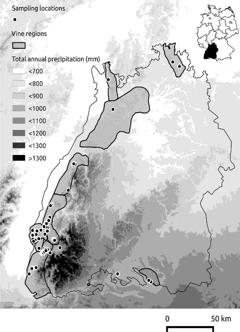
The presence of H. obsoletus was surveyed at 145 locations of its host plants (stinging nettle and/or bindweed) within the Baden region, between early June and late August 2011 (fig. 1). As planthopper flight phenology varies between years and host plants (Weintraub & Jones, Reference Weintraub and Jones2010), yellow sticky traps were placed at host plants in geographically distinct locations to constantly verify flight activity and ensure optimal sampling conditions. In addition, we used the viticulture prediction tool ‘Vitimeteo’ (www.vitimeteo.de), which estimates the flight period of H. obsoletus based on temperature sums (Maixner & Langer, Reference Maixner and Langer2006). Insect sampling was performed using a sweep net (diameter 30 cm) or a suction sampler (Stewart, Reference Stewart2002). In each of the 145 locations the selected host plant patch was surveyed only once during the sampling period. The sampling effort was proportional to patch size. Per square meter, a stinging nettle patch was swept five times, e.g., a patch of 2 m2 was swept ten times. In the presence of bindweeds, suction sampling was applied for 3 min m−2 resulting in one sample covering the entire patch. The sampling procedure was repeated after a time interval of approximately 5 min. Collected insects were transported to the laboratory, where adults of H. obsoletus were identified according to the identification keys of Biedermann & Niedringhaus (Reference Biedermann and Niedringhaus2004).

Fig. 1. 145 locations where H. obsoletus presence/ absence was surveyed as dots on a chart showing the total annual precipitation in the Baden region. Interpolated average annual precipitation was derived from the WordClim database (original spatial resolution 30 arc seconds).
Environmental predictors
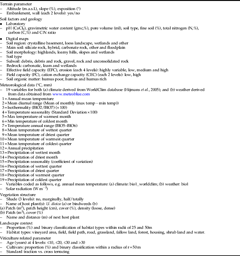
There is little quantitative knowledge about the habitat preferences of cixiid planthopper H. obsoletus. Therefore, a large set of environmental parameters (table 1) was chosen as candidate predictor variables, based on preliminary studies and general ecological knowledge. Since most species are influenced by environmental factors on different hierarchical scales (Coudun et al., Reference Coudun, Gegout, Piedallu and Rameau2006; Meyer & Thuiller, Reference Meyer and Thuiller2006), predictors operating at different spatial scales were included in this study.
Table 1. Environmental parameter recorded for all sampling locations.
Soil sample analysis
At each location a composite soil sample was obtained by collecting a combination of three sub-samples from the upper soil horizon (10 cm), using the grab sampling method. Soil texture was determined using the ‘Finger test’ (Schlichting et al., Reference Schlichting, Blume and Stahr1995; Sponagel, Reference Sponagel2005). One hundred grams of moist soil was weighed and placed in the oven for a minimum of 12 h at 105 °C (VDLUFA, 1991). Differences between moist and dried soils were used to estimate the gravimetric moisture content (gmc) according to Black (Reference Black1965). Oven-dried soils were sieved (pore size 2 mm) to assess the amount of fine soil. The soil pH (KCl) was measured in a suspension of salt solution of neutral reaction (VDLUFA, 1991). The percentages of total nitrogen and carbon were determined with the ‘elementar analyser vario MAX CN’ with 850–1150 °C following the Dumas combustion methodology (VDLUFA, 1991). In this study, the C:N ratio was calculated using the total carbon instead of Corg. In addition, three undisturbed soil samples were collected in 100 ml cylinders at all locations. The volume of the solid state body including water (ssw) was determined using a pycnometer (Danielson & Sutherland, Reference Danielson, Sutherland and Klute1986).
Finally, total pore volume (p) was calculated using the following equation:
 $${\rm p} = {\rm az - (ssw - gmc - cap),}$$
where
az = actual cylinder volume (ml)
ssw = solid state body including water (ml)
gmc = gravimetric moisture content (%)
cap = volume of standardized cylinder cap (ml)
Further edaphic parameters were derived from digital soil maps of Baden-Württemberg (scale 1:200,000) provided by the Federal State Office for Geology Resources and Mining, Freiburg Regional Board (LGRB) (table 1).
Climate and weather variables
In order to obtain biologically meaningful variables that are closely associated with a species’ physiological constraints, bioclimatic variables were used to infer the effect of both climate and weather on distribution of H. obsoletus. Interpolated climate data with a spatial resolution of 30 arc seconds were derived from the WorldClim dataset (Hijmans et al., Reference Hijmans, Cameron, Parra, Jones and Jarvis2005, http://www.worldclim.org, downloaded 8 June 2012). This dataset represents weather conditions between 1950 and 2000. Weather variables including air temperature (2 m a.g.°C) and precipitation (mm) were provided by Meteoblue (http://www.meteoblue.com) as gridded data (resolution ∼3 km) for the year 2010. Data points were interpolated using inverse-distance interpolation. In the case of temperature, simple lapse-rate adjustment was performed additionally to account for the effect of elevation in orographically heterogeneous terrain (Dodson & Marks, Reference Dodson and Marks1997). Bioclimatic variables were derived from the interpolated climatic data using the ‘biovars’ function from the R package ‘dismo’ (Hijmans et al., Reference Hijmans, Phillips, Leathwick and Elith2011).
Vegetation structure, habitat types and grapevine varieties
Information about vegetation structure included the names of the host plants, their patch size and cover, and additionally in the case of stinging nettle patch height and the compactness of the stand (loose, dense). A patch was defined as the area including all host plants with a minimum distance of 3 m to the next patch. The distance to the next host plant patch represented an indicator of patch isolation. Moreover, we recorded the potential shade intensity around midday. At each location a set of landscape context parameters were quantified using high-resolution orthophotos. Buffers with radii of 25 m and 50 m were generated within GIS to gauge the proportions of different habitat types surrounding each location (table 1).
In addition, information about the grapevine varieties and their plant years were extracted from the viticulture registry maintained by the State Institute for Viticulture and Oenology on 23rd February 2012. Quantity and expansion of different cultivars as well as the average plant age within a buffer of r = 50 m were calculated based on digital information of land parcels. Only grapevine varieties with at least five observations in the data set were considered for subsequent analysis. The orthophotos and the land parcel GIS layer were provided by the State Office of Land Consolidation and Land Development (LGL).
Statistical analysis
Model development
General linear modelling (GLM, McCullagh & Nelder, Reference McCullagh and Nelder1989) was used to develop explanatory species distribution models (SDMs). The patch occupancy of H. obsoletus was subjected to logistic GLM's by specifying a binomial error distribution and a logit link function (Hosmer & Lemeshow, Reference Hosmer and Lemeshow2000).
Model development has previously been described in detail by Strauss & Biedermann (Reference Strauss and Biedermann2006). In brief, univariate logistic regression models were first conducted for each environmental variable using all survey data. In order to account for unimodal relationships between species occurrence and environmental predictors, additional univariate models, including a quadratic term, were constructed in the case of ordinal or metric variables (Austin, Reference Austin2002). To avoid possible spurious relationships, only univariate models were retained for subsequent analysis if they met the following criteria: (i) a R 2N (Nagelkerke, Reference Nagelkerke1991) ≥0.05 (Strauss & Biedermann, Reference Strauss and Biedermann2005); and (ii) being significant at the 0.05 level.
Secondly, multivariate logistic regression models were developed for all possible combinations of candidate predictor variables. We constructed three model types (hereafter referred to as MC, MCW and MCU, respectively). The MC model type included environmental variables and climate data (from the WorldClim dataset). Models with a combination of environmental variables, climate data and weather variables as predictors were termed MCW. The MCU model type included environmental variables, climate data and additionally the height of the stinging nettle patch (‘patch_height’). To balance model overfitting and parsimony (Burnham & Anderson, Reference Burnham and Anderson2002; Franklin, Reference Franklin2009), the maximum number of combined predictors were restricted. According to the size of our data set, this number was set to four (Guisan & Zimmermann, Reference Guisan and Zimmermann2000). In order to address the issue of multicollinearity (Neter et al., Reference Neter, Wasserman and Kutner1989; Graham, Reference Graham2003), correlated variables (Spearman's r>0.7; Fielding & Haworth, Reference Fielding and Haworth1995) were not included in the same multivariate model. Significant multivariate models (P≤0.05) were considered for further analysis if they shielded (i) a R 2N (Nagelkerke, Reference Nagelkerke1991)≥0.6 and (ii) an ‘area under the curve’ (AUC) of the receiver-operating curve (ROC)≥0.9. The bioclimatic variable 12 (average annual precipitation, mm) and 13 (precipitation of wettest month, mm) were closely related. Thus, only models with the former variable were considered due to the complementary nature of both. Likelihood ratio tests were calculated for each multivariate model and its corresponding nested models to exclude the possibility of significant deviance reductions (Whittaker, Reference Whittaker1984; Ferrier et al., Reference Ferrier, Drielsma, Manion and Watson2002).
Each multivariate model was subjected to an internal validation by applying a bootstrap procedure with 1000 iterations (Verbyla & Litvaitis, Reference Verbyla and Litvaitis1989). This re-sampling technique ensures unbiased estimates of model performance (Harrell, Reference Harrell2001). Bootstrapped multivariate models were excluded if they did not exhibit an R 2N (Nagelkerke, Reference Nagelkerke1991) ≥0.5 and an AUC≥0.85 for at least 95% of the bootstraps.
Spatial autocorrelation (SAC) may lead to biased variable selection or coefficient estimation (Franklin, Reference Franklin2009). The global Moran's I coefficients were computed to examine spatial dependency of model residuals (Dormann et al., Reference Dormann, McPherson, Araujo, Bivand, Bolliger, Carl, Davies, Hirzel, Jetz, Kissling, Kuhn, Ohlemuller, Peres-Neto, Reineking, Schroder, Schurr and Wilson2007). Since we could not detect any spatial pattern in the residuals, there was no further need to take measures to address autocorrelation aspects (table 2).
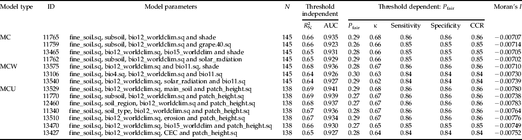
Table 2. Model performances and Global Moran's I statistics of multiple models which were used to construct average models. All performance measures represent arithmetic means as corrected by bootstrapping. ’.sq’ indicates a second order term was included to model a unimodal relationship. Model type refers to models that include besides other environmental parameters: (1) climate (MC), (2) climate and weather (MCW) and (3) climate and stinging nettle patch height (MCU). Abbr.: N = number of observations; R 2N = coefficient of model calibration; AUC (area under the receiver operating characteristic curve) = threshold independent measure for model discrimination; P fair = threshold where sensitivity equals specificity; κ = Cohen's kappa; sensitivity = proportion of correctly predicted presences; specificity = proportion of correctly predicted absences; CCR = correct classification rate; Moran's I = global test to examine spatial structures in model residuals.
The remaining models were subjected to model averaging (Burnham & Anderson, Reference Burnham and Anderson2002; Strauss & Biedermann, Reference Strauss and Biedermann2006). Model averaging calculates averaged coefficients based on the Akaike information criterion (AIC) and Akaike weights. In this study, the second order Akaike information criterion (AICc) was applied, as recommended with small datasets (Buckland et al., Reference Buckland, Burnham and Augustin1997). In applying the AICc, a set of candidate models and their predictors are evaluated to obtain an averaged model that best reflects species habitat requirements. R v. 2.13.1 software (R Development Core Team, 2011, http://www.r-project.org) was used as a simulation platform for statistical analyses.
Model performance
The degree of model performance was evaluated by using a set of criteria. Nagelkerke's (Reference Nagelkerke1991) R 2N was used as an indicator of model calibration and refinement. Values between 0 and 1 describe the variability explained by the model predictors. To access the rate of prediction error (model discrimination) threshold-dependent measures such as sensitivity (correctly predicted species presences), specificity (correctly predicted species absences) and Cohen's kappa (κ) were calculated (Cohen, Reference Cohen1960; Manel et al., Reference Manel, Dias, Buckton and Ormerod1999). The threshold was chosen to account for sensitivity and specificity in equal measure (p fair). In addition, the AUC was assessed as a threshold-independent metric of discriminative power (Hanley & McNeil, Reference Hanley and McNeil1982; Fielding & Bell, Reference Fielding and Bell1997).
Results
Prevalence and flight activity
The prevalence of H. obsoletus in the studied locations was 28%. The proportion of absences vs. presences was not significantly different between locations with only bindweeds and locations with stinging nettle alone or in combination with bindweeds (prevalence (%): 29:32:21; Fisher's exact test, P>0.05). Flight activity started in the beginning of June and ended in mid August.
Model performance
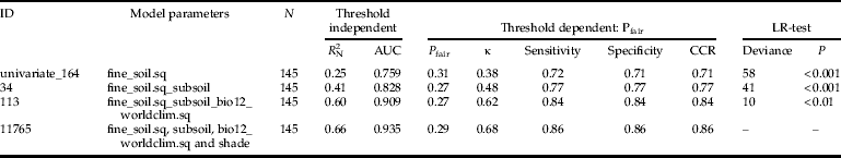
In total, 51,544 logistic regression models were built. These models consisted of 242 univariate (sigmoid as well as unimodal) and 51,302 multivariate regressions. The occurrence of H. obsoletus was explained best by multivariate models containing four environmental parameters. For example, comparison of model id = 11,765 with any model with less variables showed that the full model performed best in terms of model calibration and discrimination (table 3). Each time, the LR-test confirmed a significant deviance reduction by using the full model. Satisfying the minimum threshold criteria (R 2N≥0.6 and AUC≥0.9), four multivariate logistic models were found for the model type MC (environmental and climate data) (table 2). The inclusion of weather data from the year before the survey (model type MCW) increases model calibration (R 2N = 0.68). The highest values of model performance (calibration as well as discrimination) were achieved by including the height of stinging nettle patch as an additional parameter (model type MCU, R 2N = 0.69, AUC = 0.941). With regard to the discriminatory abilities using threshold-dependent criteria, all selected multivariate logistic regressions exhibited correct classification rates ranging between 84 and 86% (table 2). Cohen's κ values ranged between 0.62 and 0.68 (table 2).
Table 3. Comparison of a four parameter model with all corresponding nested correspondents. All performance measures represent arithmetic means as corrected by bootstrapping. ’.sq’ indicates a second order term was included to model a unimodal relationship. Abbr. see table 2.
Relative importance of environmental parameters
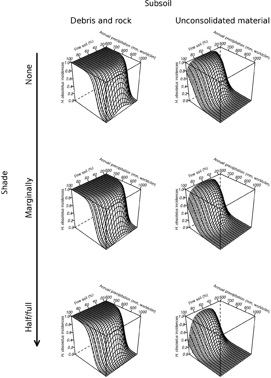
Three average models were developed for the following model type combinations: (1) MC; (2) MC+MCW; and (3) MC+MCU. Regardless of different ecological assumptions, all average models demonstrated that the potential habitat of H. obsoletus is largely characterized by the amount of both fine soil and average annual precipitation. The percentile weights of both variables remained consistent across all average models (tables 4–6). These two variables are unimodal related to the planthoppers occurrence, whereas occurrence probabilities are highest with an intermediate level (∼60%) of fine soil from the upper soil layer and a low amount of average annual precipitation (fig. 2). Furthermore, fig. 2 depicts that H. obsoletus preferred marginal or no-shaded host plant patches. The occurrence of the planthopper is also related to soil geology, particularly to the type of subsoil (fig. 2). Shade and the subsoil type together account for 28 and 27% of the total percentile weight (tables 4 and 6). In addition, on including the weather data, the effect of these two variables on species occurrence is replaced by bio11 (mean temperature of the coldest quarter) (table 5). As shown by the coefficients of the average model in table 6, occurrence probabilities of H. obsoletus are highest in patches of U. dioica with low host plant height. In contrast to edaphic or climate- and weather-related factors, terrain variables as well as the landscape context have no or little impact on species occurrence.
Fig. 2. Average model MC (environmental and climate data) for H. obsoletus. The probability of occurrence of H. obsoletus is plotted against the amount of fine soil and average annual precipitation; diagrams represent different levels of shade and two categories of subsoil (other subsoil categories showed a similar trend as ‘unconsolidated material’ and are, therefore, not shown).
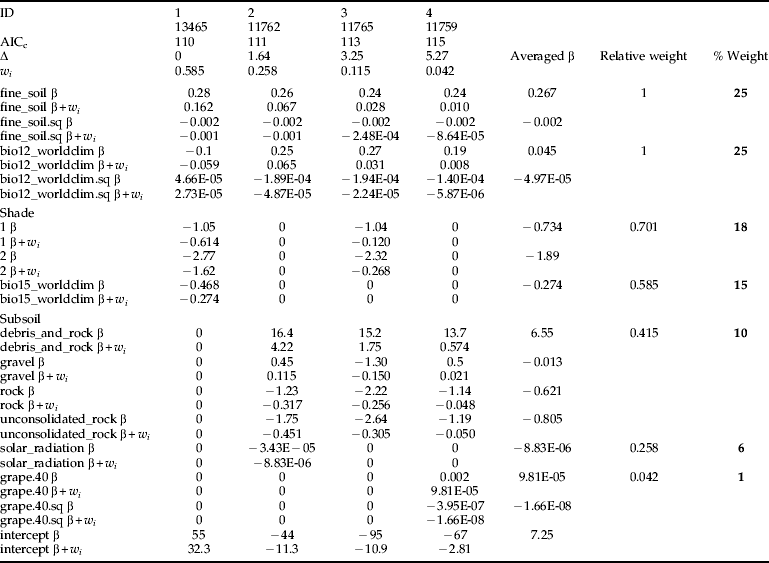
Table 4. Model averaging using four multiple models from the MC model type of table 2. Models were ranked in descending order according to their AICc. For each model weights (w i) were calculated based on AICc differences (Δ) and were used to derive individual coefficients weights (β×w i) in the next step. Finally, averaged coefficients (averaged β) and variable weights (relative and percentile) were determined.
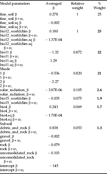
Table 5 Model averaging using multiple models from the “worldclim” model type (MC) combined with models from the “worldclim + weather” model type (MCW) of table 2. Variables with a percental weight lower than one are not shown.
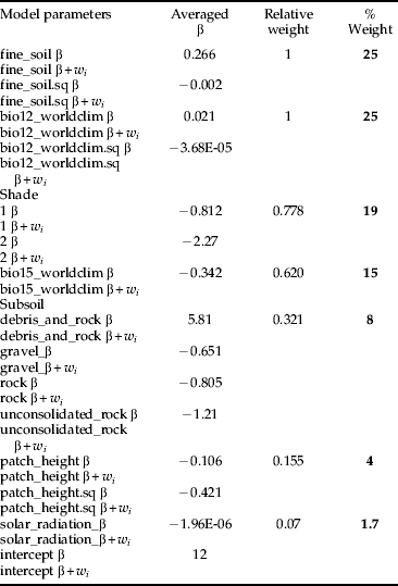
Table 6. Model averaging using multiple models from the “worldclim” model type (MC) combined with models from the “worldclim + stinging nettle patch height” – model type (MCU) of table 2. Variables with a percental weight lower than one are not shown.
Discussion
Multivariate effects of environmental parameters on distribution of H. obsoletus
We were able to build species distribution models (SDMs) including a variety of environmental predictors based on ecological expertise and previous literature studies. Furthermore, three different average models based on multivariate logistic regressions provided multiple lines of evidence identifying and quantifying the habitat preferences of H. obsoletus. In agreement with different habitats associated with different life stages of the soil-borne planthopper, our results indicate that (1) H. obsoletus occurrence is best characterized by a combination of multiple environmental parameters; and (2) the influence of the main environmental drivers appears to be twofold: above as well as below ground.
Soil conditions are reported to significantly influence leafhopper assemblages (Sanderson et al., Reference Sanderson, Rushton, Cherrill and Byrne1995; Strauss & Biedermann, Reference Strauss and Biedermann2006). The influence of soil texture on nymphal development of H. obsoletus was already suggested by different authors (Maixner & Langer, Reference Maixner and Langer2006; Lessio et al., Reference Lessio, Tedeschi and Alma2007; Cargnus et al., Reference Cargnus, Pavan, Mori and Martini2012). With respect to H. obsoletus, the modelling results suggest that soil properties related to the pore matrix influence occurrence probabilities. Our analysis identified the amount of fine soil in the upper 10 cm of the soil and the subsoil as highly influential variables, both characterizing the soil pore system. In contrast to argillaceous soils with a dense pore matrix and low pore volume, soils with a coarse pore matrix and low water retention capacity seem to be preferred by H. obsoletus.
The dynamics of insect populations are highly influenced by climate and weather variables (Porter et al., Reference Porter, Parry and Carter1991; Cammell & Knight, Reference Cammell and Knight1992; Cannon, Reference Cannon1998; Huffaker & Gutierrez, Reference Huffaker and Gutierrez1999; Sforza et al., Reference Sforza, Bourgoin, Wilson and Boudon-Padieu1999). Yet, few studies have evaluated the potential effect of temperature and precipitation on Auchenorrhyncha populations (Biedermann et al., Reference Biedermann, Achtziger, Nickel and Stewart2005). Recent studies including Diptera species revealed that the effect of rainfall and humidity, respectively, is often controversial and species specific (Juliano et al., Reference Juliano, O'Meara, Morrill and Cutwa2002; Duyck et al., Reference Duyck, David and Quilici2006). Our study shows a strong negative relationship between average annual rainfall and occurrence of H. obsoletus at the spatial extent of the Baden region. Interestingly, temperature did not represent a main environmental factor driving the occurrence probabilities of H. obsoletus. This does not necessarily mean that species occurrence is unrelated to temperature but that temperature probably acts on a different scale or is indirectly represented by other variables. Hence, clear differences of H. obsoletus occurrence probabilities between locations, characterized by different degrees of shade, may indicate a high influence of micro-climatic conditions. Factors affecting the micro-climate such as vegetation structure and shade were shown to significantly affect the occurrence of Auchenorrhyncha in a habitat modelling study (Biedermann, Reference Biedermann2004). We further assumed that variation in weather conditions in the year preceding the planthopper survey affect species occurrence. This hypothesis is supported by Whittaker & Tribe (Reference Whittaker and Tribe1998) stating that the mean minimum temperature of September highly influences the population density of the spittlebug Neophilaenus lineatus (L.) (Homoptera, Auchenorrhyncha) in the following year. The average model MC+MCW (model with climate and weather variables) highlights that additional knowledge about habitat preferences can be obtained by not only focusing on long-term climate changes but also incorporating short-term weather events. This way, specific traits of certain species such as feeding or oviposition preferences related to occurrence characteristics might be revealed. In our study, the weather variable bio11 (mean temperature of coldest quarter of the year 2010) received a high percentile weight in the average model MC+MCW, replacing the climate variable bio15_worldclim (precipitation seasonality) and subsoil from the average model MC (model with climate variables only). Denno & Roderick (Reference Denno and Roderick1990) stated that the survival of planthoppers overwintering as nymphs is negatively correlated with winter severity. In contrast, the high ranking of bio11 suggests that the nymphs are not primarily susceptible to the rigours of a harsh winter. Many overwintering insects tolerate winter severity by migrating into deeper soil layers (Leather et al., Reference Leather, Walters and Bale1993). Maixner (Reference Maixner, Weintraub and Jones2010) found that at the northern range border nymphs of H. obsoletus are able to avoid frost damage by escaping into a soil depth of 20–25 cm. Moreover, bio11 is negatively correlated with the occurrence of H. obsoletus. We have no straightforward ecological explanation for this phenomenon. The planthoppers’ preference for locations with low temperature during the coldest quarter might be related to indirect effects on predators or parasites.
Furthermore, we found that in patches with low host plant height occurrence probabilities of H. obsoletus were significantly increased. Thus, stinging nettle patches in managed landscapes with regular mowing of embankments and field margins seem to provide a suitable ecological niche in the Baden region.
Effects of agricultural management practices on interpretation of SDMs
The application of SDMs can be compromised by several limitations in agricultural studies. These are due to the inherent dynamics of these study systems. In addition to natural environmental variation, agricultural management practices introduce high variability in a dataset used to study crop pests (Altieri, Reference Altieri1999; Duyck et al., Reference Duyck, Dortel, Vinatier, Gaujoux, Carval and Tixier2012; Guerra & Steenwerth, Reference Guerra and Steenwerth2012). Maps of habitat types used to quantify the surrounding landscape context may differ from one year to another, which is probably due to abandoned farmland or the cultivation of different types of field crops.
With respect to leaf – and planthoppers, the importance of the distribution and structure of the host plant(s) was highlighted by several authors (Denno & Roderick, Reference Denno and Roderick1990; Zabel & Tscharntke, Reference Zabel and Tscharntke1998; Biedermann, Reference Biedermann2002). However, vegetation mowing or the application of herbicides alter host plant related parameters such as patch size or patch height. One solution might be the usage of an extensive data set as demonstrated by Duyck et al. (Reference Duyck, Dortel, Vinatier, Gaujoux, Carval and Tixier2012). Another approach was presented in this study using different average models. Taking into account a reliable dataset based on a reasonably high number of sampling records, we could identify a possible negative relationship between stinging nettle height and species occurrence probabilities. This average model (MC+MCU), however, is associated with some degree of uncertainty due to the above mentioned reasons. Therefore, for prediction purposes, the use of model types MC and MCW, respectively, would be preferred.
The use of SDMs in agricultural risk analysis – opportunities and limitations
SDMs are well-established tools in many fields of biological research (Dormann et al., Reference Dormann, Blaschke, Lausch, Schröder and Söndgerath2004; Guisan & Thuiller, Reference Guisan and Thuiller2005). Despite their popularity and their advantages, only few studies have successfully applied SDMs in agricultural risk analysis (e.g., Meentemeyer et al., Reference Meentemeyer, Rizzo, Mark and Lotz2004; Hamada et al., Reference Hamada, Ghini, Rossi, Júnior and Fernandes2008). On the one hand, pest management strategies could highly benefit from increased knowledge about the habitat requirements of many crop pests. In viticulture, detailed ecological information about major grapevine pests such as the grape berry moths Eupoecilia ambiguella Hb. and Lobesia botrana Schiff. or virus vectoring nematodes is still lacking. On the other hand, SDMs can be used to derive predictions of the potential distribution of crop pests. Such predictive maps may equally help farmers and decision makers to identify areas at high risk and to initiate appropriate plans of action. New avenues of research provide the geographical range prediction of invasive species. An example is the leafhopper Scaphoideus titanus Ball., the vector of the grapevine yellows disease Flavescence doreé (Schvester et al., Reference Schvester, Carle and Moutous1963). This species expands its geographical range in Europe towards north at an alarming spread (Boudon-Padieu & Maixner, Reference Boudon-Padieu and Maixner2007). Spatial extrapolations of previously developed SDMs could be a useful technique to identify suitable habitats. However, predictive maps of spatial extrapolations should be interpreted with a certain degree of caution and be subjected to a critical analysis as shown by De Meyer et al. (Reference De Meyer, Robertson, Mansell, Ekesi, Tsuruta, Mwaiko, Vayssières and Peterson2010). Applying two modelling approaches, the authors predicted that suitable habitats of the invasive fruit fly, Bactrocera invadens (Diptera: Tephritidae), are characterized by high temperatures and a humid environment. Independent distributional data confirmed the robustness of the model predictions, nevertheless these predictions did not cover all known occurrences. Such discrepancies might be attributable to several factors such as (1) the spatial extrapolation was applied outside the environmental space used to develop the SDM (Franklin, Reference Franklin2009), or (2) a niche shift occurred as demonstrated for some species (Broennimann et al., Reference Broennimann, Treier, Muller-Scharer, Thuiller, Peterson and Guisan2007; Fitzpatrick et al., Reference Fitzpatrick, Weltzin, Sanders and Dunn2007; Steiner et al., Reference Steiner, Schlick-Steiner, VanDerWal, Reuther, Christian, Stauffer, Suarez, Williams and Crozier2008).
SDMs are usually based on the assumption of pseudo-equilibrium (Guisan & Theurillat, Reference Guisan and Theurillat2000), since ecological surveys mostly represent snapshot views of ecological patterns of species-environment relationships. This assumption hampers the straightforward application of SDMs on species exhibiting range expansions or recently introduced species. An example in the Baden region is Drosophila suzukii Matsumura, a recently fast spreading fruit fly (Breuer, unpublished data; Cini et al., Reference Cini, Ioriatti and Anfora2012). In these cases, the invasive species may not yet be in equilibrium with the environment. However, new methodological frameworks are now proposed to deal with such non-equilibrium dynamics (e.g., De Marco et al., Reference De Marco, Diniz and Bini2008; Gallien et al., Reference Gallien, Douzet, Pratte, Zimmermann and Thuiller2012).
With respect to H. obsoletus, insect pest management is currently based on biomonitoring in combination with a phenological model using temperature sums (Maixner & Langer, Reference Maixner and Langer2006). Yet, biomonitoring is laborious and time consuming and thus is limited in practice. Information about flight activity without knowing the species’ ecological habitat preferences and occurrence probabilities may result in ineffective pest control measures. Adverse effects on non-target organisms and many aspects of ecosystem functioning due to the inappropriate application of pesticides are well documented (for a review in viticulture see: Guerra & Steenwerth, Reference Guerra and Steenwerth2012). In this context, the developed SDMs are of high relevance in viticulture and can be further used to predict the planthoppers potential distribution in the vineyards of the Baden region. In the long term, both the phenological model and the SDMs may provide a complete picture about the spatio-temporal occurrence of H. obsoletus and thus, support integrated pest management strategies. Here, we exemplified the analysis of habitat requirements using SDMs for a crop insect in viticulture, an approach that can be easily adopted to other crop pests and diseases.
Acknowledgements
The work was financed by the Association of German Wine scientists (FDW). The authors are very grateful to Elke Friebe, Werner Weinzierl and Karl G. Gutbrod for providing area-wide GIS data. We thank Gabriele Trefz-Malcher for providing a pycnometer and related technical support. Many thanks to our colleagues from the State Institute of Viticulture and Oenology (WBI), especially to the entire soil department group; Sabine Oster and Patricia Bohnert for their field work assistance; and Carsten Schmidt, Patrik Kehrli, Michael Maixner and two anonymous reviewers for valuable comments on the manuscript.