Introduction
In wireless communication systems antenna is an important component that is used to transmit and receive electromagnetic waves. As there is a great demand for small, lightweight, and portable telecommunication systems, therefore, various fractal geometries have been studied and analyzed to reduce the size of these systems. Fractals are very complex and these structures are generated with the use of iterative method [Reference Arya, Khan, Shan and Lehana1, Reference Arora, Kumar, Khan and Arya2] which follows a simple process repeated many times. In the first time, Mandlebort [Reference Wong3] reported a fractal structure that is extensively used in designing antennas. Different types of fractal fragments have been defined in the literature [Reference Baliarda, Robert, Pous, Ramis and Hijazo4–Reference Bisht and Kumar8]. Despite these fractal geometries, various fractal structures are based on a square curve [Reference Bangi and Sivia9]. These fractal designs follow a self-similar and space-filling procedure [Reference Kaur and Sivia10–Reference Bhatt, Mankodi, Desai and Patel12] under which the same iteration factor is used at a different scale. Antenna performance parameters are also affected by the selection of the ground plane. Variation in ground plane size affects the radiation characteristics of the antenna. A square shape antenna has been designed and antenna characteristics such as return loss, gain, and half power beam width have been described to study the effect of the ground plane on antenna performance.
A single antenna is not sufficient to increase the gain or directivity. Therefore, many fractal antennas are joined at a particular distance to enhance radiative properties. These antenna elements are excited in such a way that each element gives the same amplitude of the current. These antenna array patch elements can be arranged in a linear [Reference Lakshmana Kumar, Satyanarayanana, Sridevi and Parakash13] manner or in a planar way [Reference Barison, Deo and Syahkal14]. Antenna array provides better impedance matching. Different feeding techniques [Reference Errifi, Baghdad, Badri and Sahel15] can be used to excite an antenna array. In a corporate feeding technique, a λ/4 transformer is used for impedance matching of an antenna array. Various fractal antenna arrays have been described in the literature [Reference Pal, Roy, Nag and Tiwary16, Reference Bernety, Gholami, Bijan Z and Rastamian17] with series and corporate feeding methods for different materials. High directivity and narrow radiation pattern of antenna array increase use in various applications.
From the last few years, artificial neural network (ANN) has become very popular for solving various engineering [Reference Kumar and Singh18] problems. Neural networks have been used to design [Reference Sivia, Pharwaha and Kamal19] microstrip antenna arrays. Four algorithms of the ANN have been described to design rectangular microstrip antenna [Reference Singh20]. A comparative analysis has been done and it has been concluded that the radial basis function algorithm achieves minimum error for resonant frequency [Reference Sivia, Pharwaha and Kamal21, Reference Singh and Singh22]. A mathematical model has been developed for input and output variables [Reference Sivia, Singh and Kamal23] and trained with hidden layer neurons to achieve minimum error. Estimated parameters [Reference Sivia, Pharwaha and Kamal24] are compared with simulated parameters and error is calculated. It solves complex problems with greater accuracy. An E-shaped fractal antenna array [Reference Pal, Roy, Nag and Tiwary16] and spidron shape 2 × 2 antenna array [Reference Van, Kim, Kwon and Hwang25] have been considered in literature. Despite these, various researchers have reported [Reference Narayana, Krishna and Reddy26–Reference Xiao, Shao, Jin and Wang29] analysis of microstrip antenna parameters such as directivity, antenna efficiency and resonating frequency with an artificial neural network. So neural networks are an efficient tool to design and optimization of antenna parameters.
In the presented work 1 × 4, fractal array antenna with different substrate materials has been considered and simulated with HFSS software. For the estimation of designing and output parameters, a virtual instrument model has been designed in which graphical programming language is used for monitoring of input and output parameters [Reference Chengqun30, Reference Shujiao31]. Firstly, designing parameter radius has been estimated with virtual instrument model. Then estimation of output parameters such as frequency, gain, and voltage standing wave ratio (VSWR) have been done with the proposed model for input parameters, the radius of a circular patch, the height of the substrate, and dielectric constant of the material. Neural network code has been embedded in the designed model and results have been displayed in the front panel window of the proposed model.
Fractal antenna array
In the proposed work 1 × 4 fractal array antenna of circular-shaped elements has been designed with a 4.4 dielectric constant of FR-4 material on a substrate of size 54.9644 × 212.5 × 1.6 mm3. In the design of array, a λ/4 transformer has been used for the impedance match of a 50 Ω feed line with a patch as real and imaginary parts of input impedance are 52.1800 Ω and −3.2229 Ω, respectively. A defected ground plane (23.7644 × 212.5 mm2) has been used to achieve the desired frequency. With HFSS software proposed array antenna has been simulated and performance parameters are analyzed. Dimensions of proposed geometry are calculated with the following equations 1 and 2.


where d, fr ,vo , and ae are known as the dielectric constant of the material, resonant frequency, speed of light in air, and effective radius of patch, respectively. Design sequence of fractal antenna array has been described below:
-
Step 1. A Circular shape patch with a radius of 15 mm is a basic structure which is known as 0th iteration. A 50 Ω microstrip line feed of width 3.0678 mm has been used to match the impedance with a designed patch.
-
Step 2. In the first iteration, a circle of radius 5 mm is cut from the center of a circular patch which is surrounded by four circles of radii 1.66 mm. For each circle iteration factor of 1/3 has been used for the radius of each circle.
-
Step 3. In the second iteration, the same process has been repeated. Now each circle of radii 1.66 mm has been surrounded by four circles of radii 0.55 mm. As the number of iterations is increasing resonant frequency has been shifted towards the lower side. A fractal array antenna has been constructed along with four circular patches by a corporate feed network and the proposed array has been simulated through HFSS software. Proposed 1 × 4 fractal antenna array and output results have been shown in Figs 1–4.
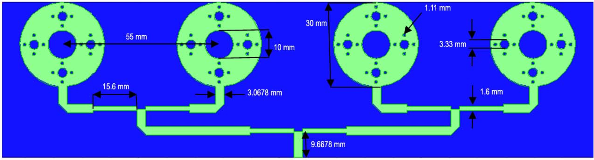
Fig. 1. Fractal antenna array.
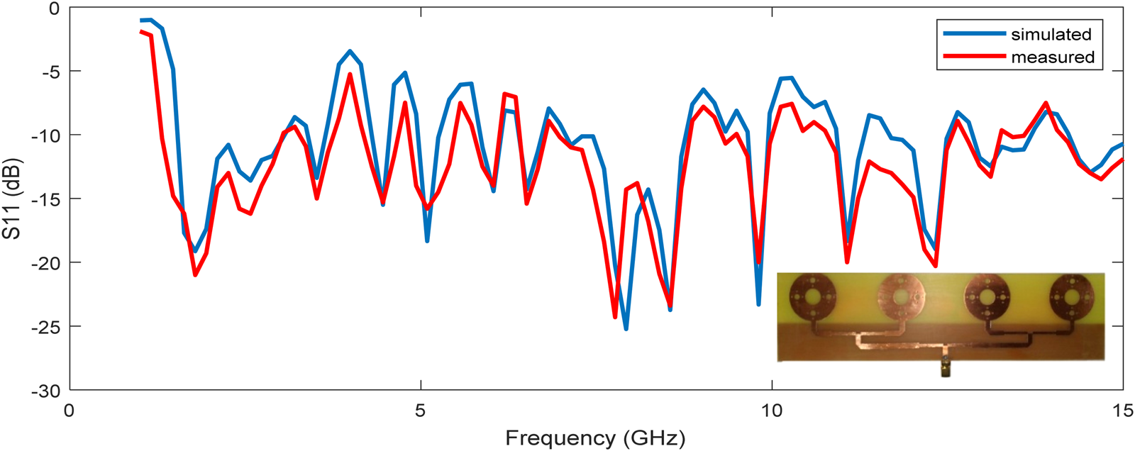
Fig. 2. S11 (dB) vs. frequency (GHz).
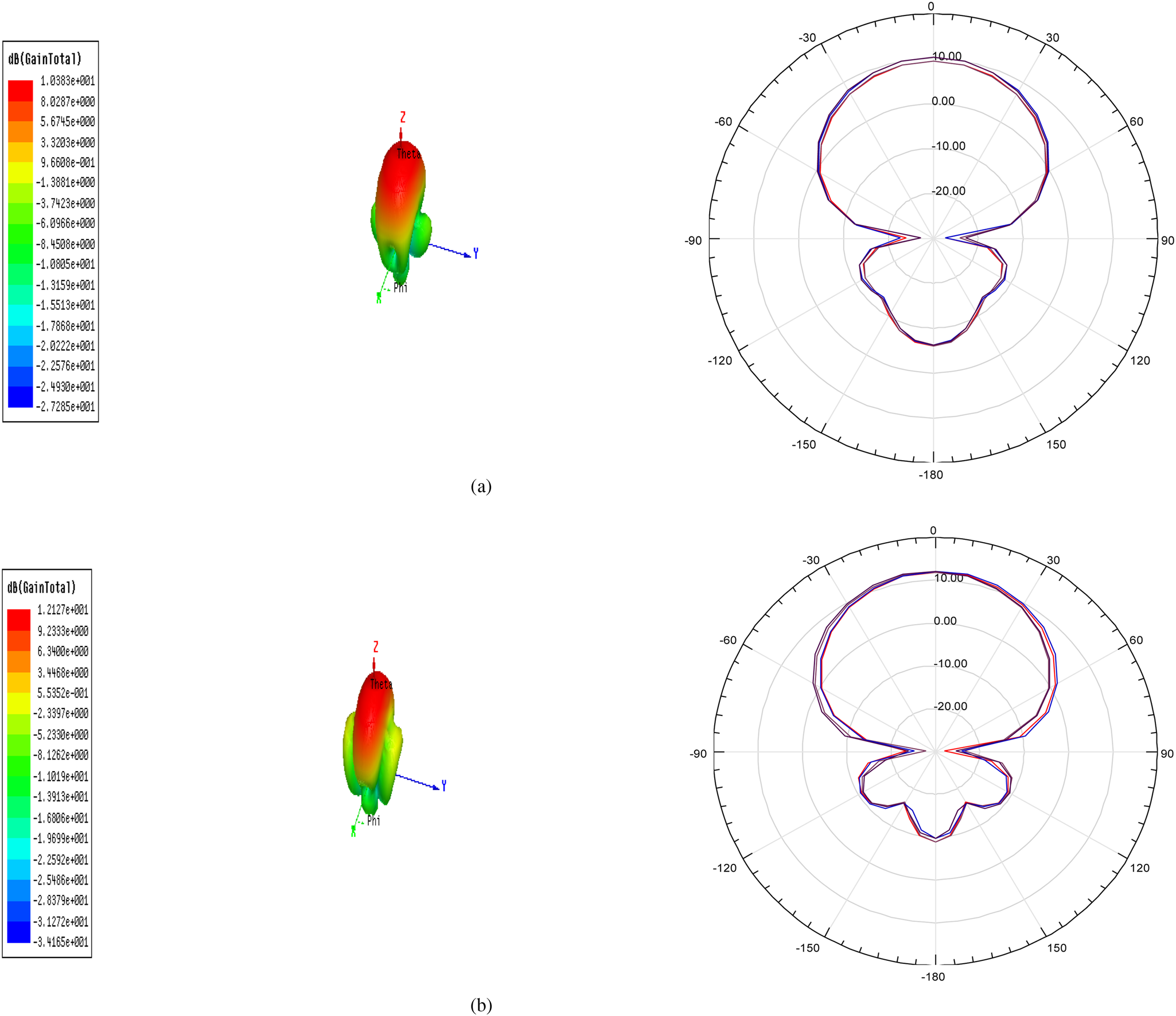
Fig. 3. Gain and radiation pattern at frequency (a) 1.7865 GHz (b) 2.5730 GHz.

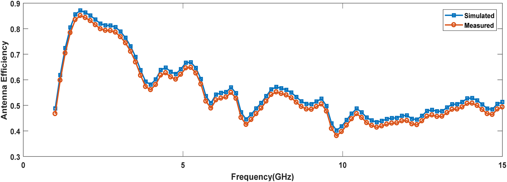
Fig. 4. Antenna efficiency vs. frequency (GHz).
From the above results, it has been observed that antenna array shows multiband response and values of measured gain have been achieved 10.383 and 12.127 dB at 1.7865 and 2.5730 GHz frequency, respectively. Antenna efficiency of 83.17 has been achieved.
Parameter estimation of fractal antenna array
A virtual instrument model has been proposed for designing and output parameter estimation of fractal antenna array. Present work includes generation and collection of data samples, development of virtual instrument model, results, and discussion.
Generation and collection of data samples for designing parameter
For the preparation of the data dictionary, different samples have been generated with a change in input parameters. For the analysis of designing a parameter (radius of the circular patch), different substrate materials with relative permittivity (d) of 4.4, 4.5, 4.8, 5.5, 5.7, 5.75, and 6.0 have been selected. For each substrate material radius of a circular patch (a) has been calculated mathematically by using equations 1 and 2 with various substrate heights (h) values changing from 1.6 to 2.0 mm. All these samples of radius have been collected and a data dictionary has been prepared with all these samples. In this prepared data dictionary different samples of input parameters such as dielectric constant (d) and height (h) of the substrate have been considered as inputs and radius of the circular patch (a) has been described as an output parameter. The pictorial representation has been given in Fig. 5.

Fig. 5. Representation of input and output parameters.
Generation and collection of data samples for output parameters
For the analysis of output parameters, a fractal antenna array, with different substrate material of dielectric constant (d) 4.4, 4.5, 4.8, 5.5, 5.7, 5.75, 6.0, substrate height (h) from 1.6 to 2.0 mm and calculated radius (a), has been designed and simulated with HFSS software and values of output parameters such as gain (g1, g2) and VSWR (v1, v2) have been obtained at (f1, f2) resonant frequencies. For each combination of input parameters (d, h, a) five samples have been generated. As seven substrate materials have been used, therefore a total of 35(5 × 7) samples have been created. All these samples of frequency, gain, and VSWR have been collected. In Fig. 6 Input parameters (d, h, a) and output parameters (f1, f2, g1, g2, v1, v2) have been represented.
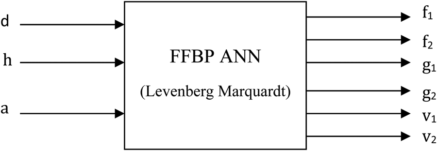
Fig. 6. Representation of input and output parameters.
Proposed work
In the proposed work virtual instrument has been designed in laboratory virtual instrument engineering workbench (LabVIEW) software which provides an engineering workbench that uses graphical language and displays the information about input and output parameters in the display window [Reference Rani and Sivia32].
Development of virtual instrument model for estimation of designing parameter
In the present work, a virtual instrument model has been developed in Lab VIEW for the estimation of designing parameter. It is consisting of numeric arrays, MATLAB script with ANN implementation, cluster, graphic indicator and MS Office Report as shown in Fig. 7.
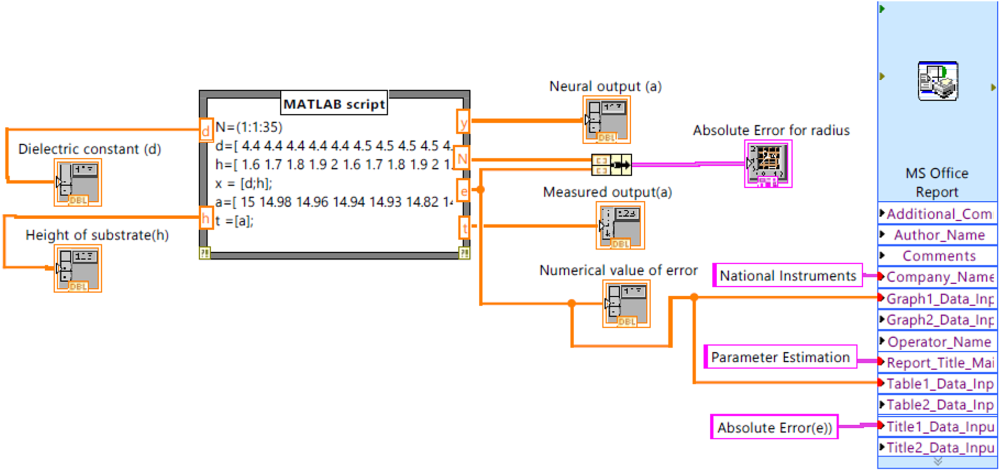
Fig. 7. Proposed virtual instrument model.
In the developed model the function of numeric array is to display the input and output parameters. MATLAB script node contains ANN code with input and output variables. Cluster is consisting of two inputs and one output and graphic indicator displays the graph for absolute error. As error output from MATLAB script node is given as input to MS Office Report generator for graph and table of absolute error. MS Office Report generator creates a report with title of report, graph and table of parameters in excel format and it can be saved for record purpose. In present work designing parameter of proposed antenna array has been estimated but multiple sub vi's can be created within a loop in main vi design and on the priority basis these sub vi's will be executed. In the MATLAB script d and h are considered as input variables and t, y, e are output variables. Variables d and h are known as dielectric constant and height of substrate as input and t, y, e are representing target, neural output, and error between target and estimated output, respectively. The neural network code has been embedded for estimation of designing parameter. In the artificial neural network, 35 data samples for inputs and outputs have been used. Out of 35 samples 70% (25 samples) in favor of training, 15% (5 samples) in support of validation, and the other 15% (5 samples) for testing have been used. In the designed network input layer is associated with two neurons, the hidden layer with 10 neurons and an output layer with one neuron. A Developed neural model has been trained with 10 hidden layer neurons to achieve minimum error so that a perfect correlation between measured and neural network outputs can be obtained. Numerical values of inputs and outputs with error have been presented in a display window of the developed virtual instrument model as shown in Fig. 8.
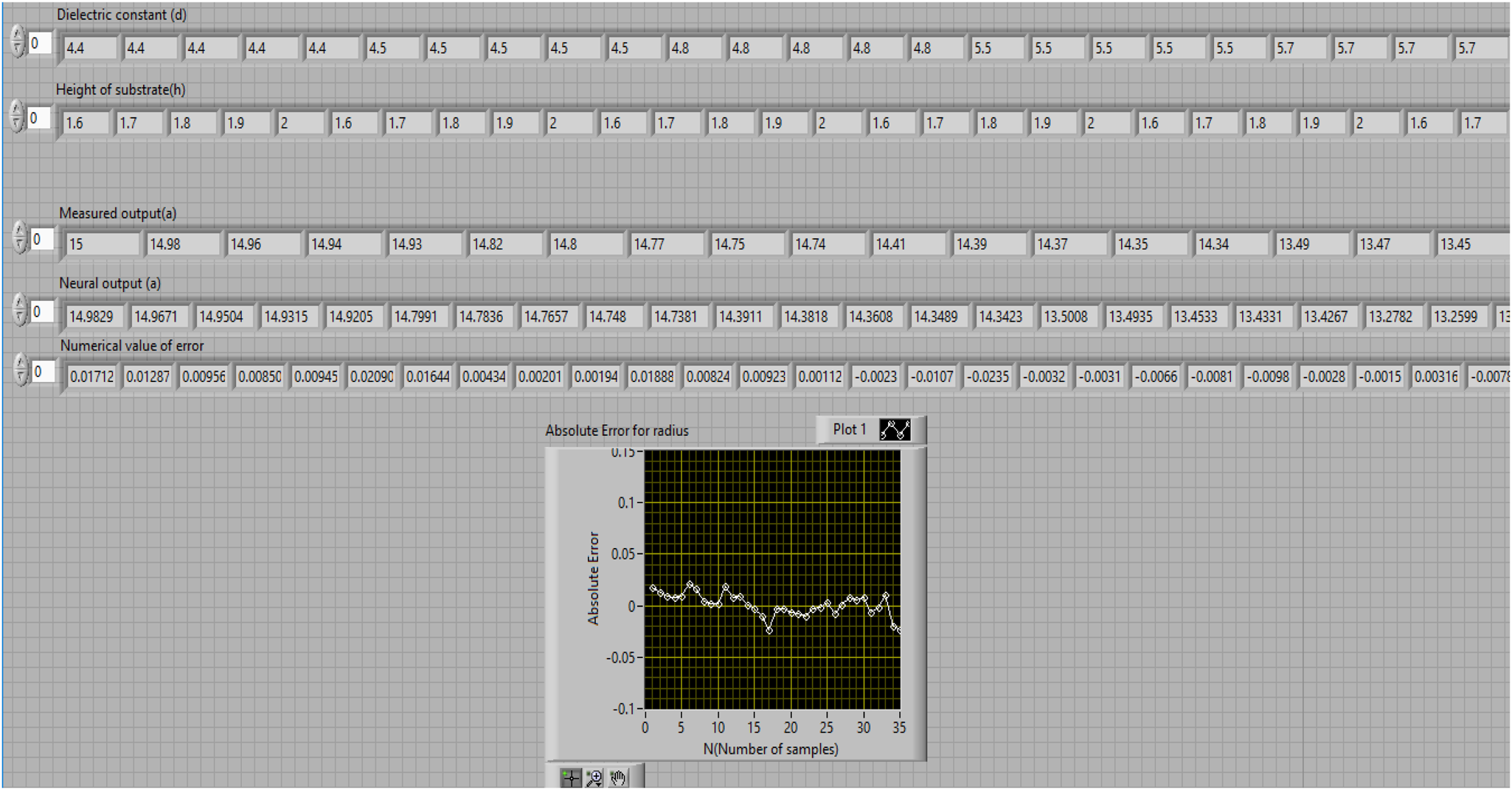
Fig. 8. Display window with inputs, outputs and error.
From the output display window, it has been observed that input parameters (d, h), output parameter (calculated a) and neural output (a) have been displayed along with error.
From simulated results it has been observed that inputs dielectric constant, height of substrate and neural outputs has been displayed. A graphical representation for absolute error between the calculated radius and estimated radius has been shown. Numerical values of measured output and neural output with error have been presented in Table 1 for the radius of a circular patch.
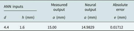
Table 1. Numerical values of inputs and outputs with absolute error.

From Table 1 it has been observed that the estimated value of radius 14.9829 mm and an absolute value of error 0.01712 mm has been achieved.
Development of virtual instrument model for estimation of output parameters
For estimating output parameters such as frequency, gain, and VSWR of a fractal antenna array, a virtual instrument model has developed in LabVIEW. It is consisting of numeric arrays, MATLAB script, index array, bundle cluster array, and graphs as shown in Fig. 9.
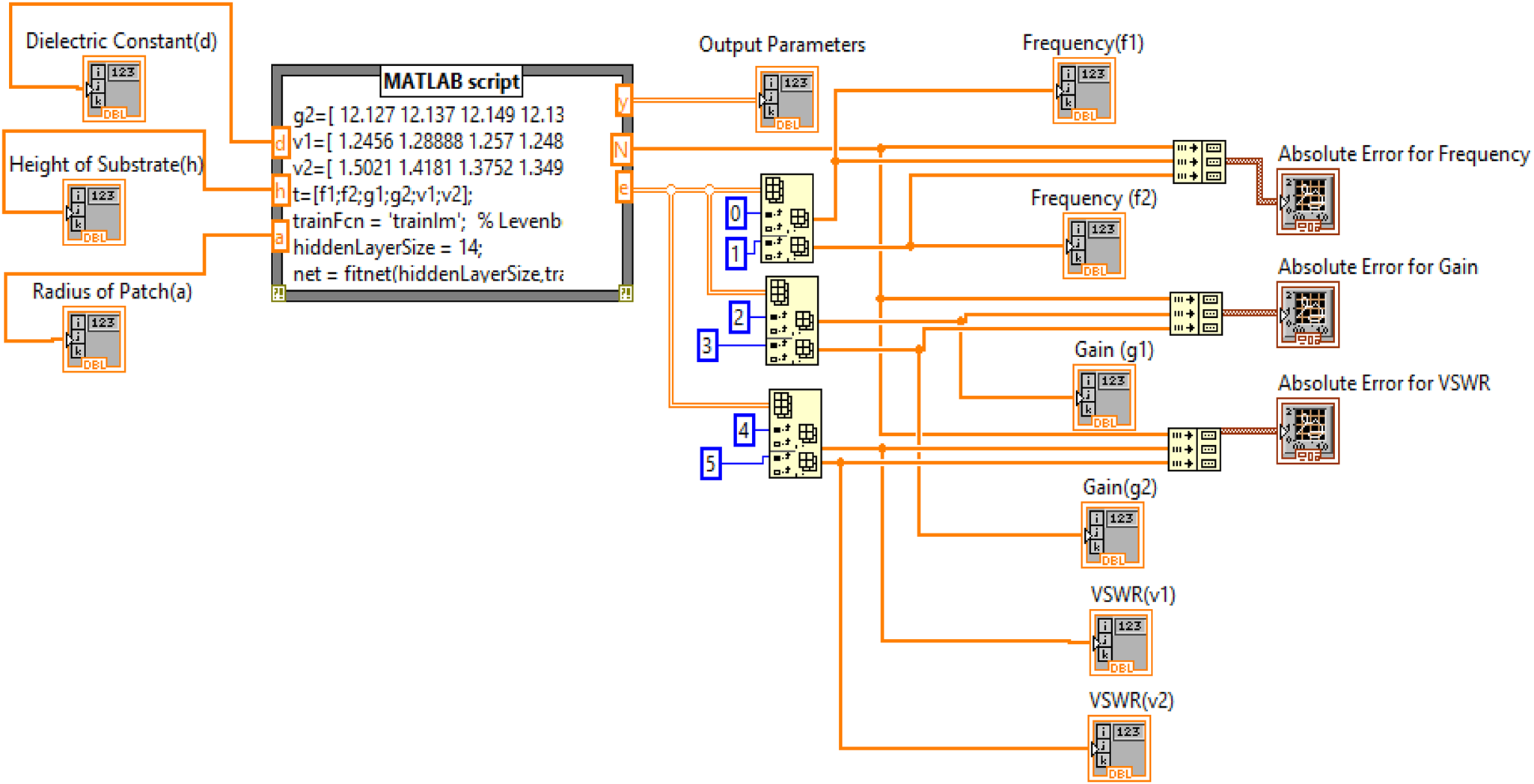
Fig. 9. Proposed virtual instrument model.
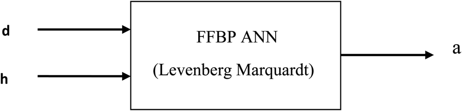
For estimating output parameters, MATLAB script is containing three input parameters as dielectric constant (d), substrate height (h) and radius of circular patch (a) and six output parameters as frequency (f 1, f 2), gain (g 1, g 2) and VSWR (v 1, v 2). The neural network code has embedded in MATLAB script. The input layer consisting of three input neurons and the output layer is associated with six neurons. Levenberg–Marquardt algorithm is used to train the network which works in feed-forward back propagation mode shown in Fig. 10.
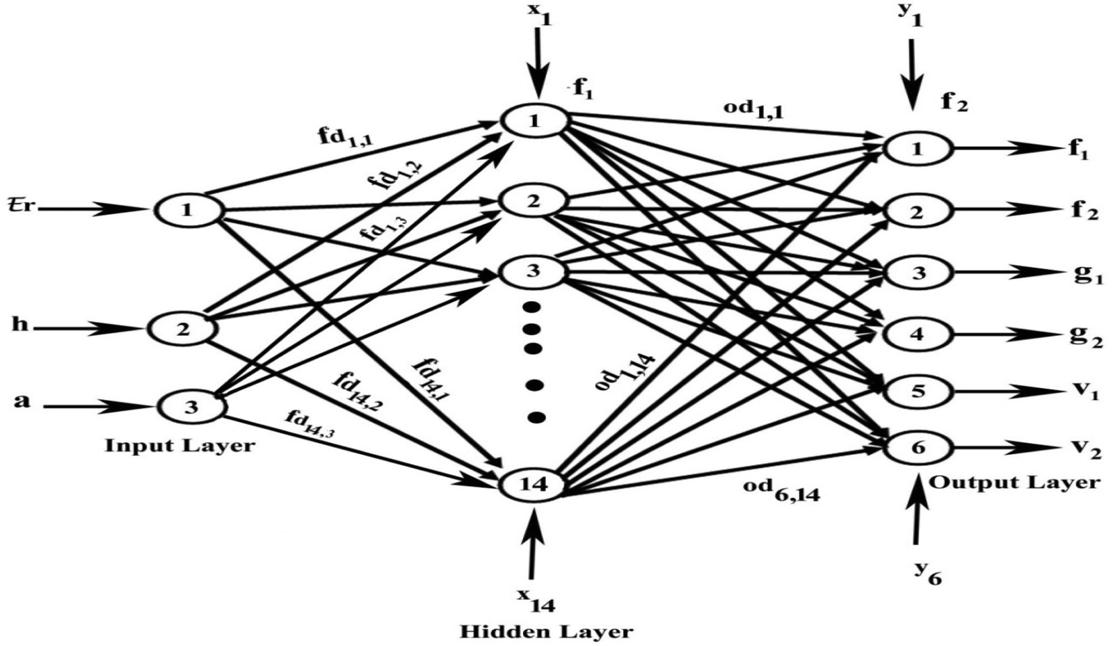
Fig. 10. Designed artificial neural network.
A mathematical analysis describes the flow of information from input side neurons to output side neurons through neurons in the middle layer.

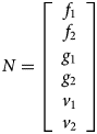
Equations 3 and 4 represent M as input and N as output matrices consisting of three input parameters which are permittivity(d), the height of material (h) and radius of a circular patch (a) and N is consisting of output parameters which are frequencies f 1, f 2, gain g 1, g 2, and VSWR v 1 and v 2.
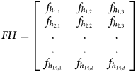
Equation 5 represents a matrix FH which shows the flow of information from input side layer neurons to middle layer neurons. It is known as weight matrices for the hidden layer.
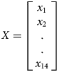

Equations 6 and 7 represent matrices X and Y. Matrix X consisting of x 1, x 2,……..,x 14 which are known as bias values for hidden layer neurons. Matrix Y consisting of y 1, y 2, y 3, y 4, y 5, y 6 which are considered bias values for output layer neurons.
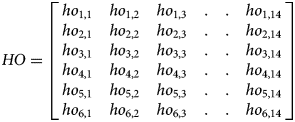
Matrix HO (equation 8) shows the flow of neurons from the hidden layer to the output layer. It is known as a weight matrix for the output layer.

In equation 9, N is represented as an output equation in which f 1 is non-linear and f 2 is a linear function at hidden and output layer, respectively.
To achieve minimum error developed model has been simulated with 14 neurons at the hidden layer which lies in between the input and output layer. After training the designed network, the neural output values of frequency, gain, and VSWR have been achieved. It is simulated again to achieve minimum error (e) between measured (t) and neural outputs (y) so that a perfect correlation has been obtained. Output results have been displayed in Fig. 11.
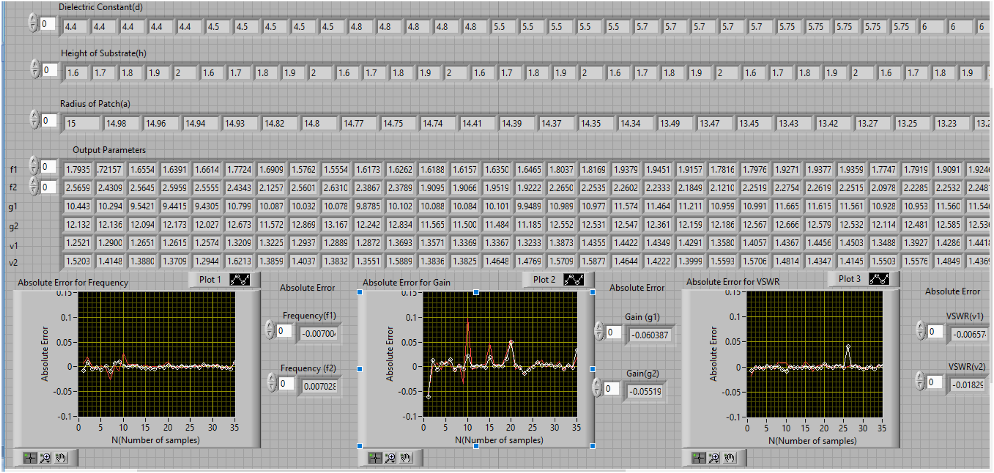
Fig. 11. Display window with inputs, outputs and error.
After simulation of designed virtual instrumentation model input and output parameters have been displayed along with the error graphically. Plot 1, plot 2 and plot 3 represent values of absolute error for frequency (f1,f2), gain (g1,g2), and VSWR (v1,v2) respectively. A comparison of measured and neural output values has been presented in Table 2.
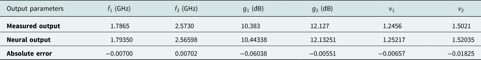
Table 2. Comparison of measured and neural outputs.

From comparison of measured and neural outputs it has been observed that absolute values of error are −0.00700 GHz, 0.00702 GHz, −0.06038 dB, −0.00551 dB, −0.00657 and −0.01825 for frequency (f 1, f 2), gain (g 1,g 2) and VSWR (v 1, v 2), respectively.
At the end performance of feed-forward back propagation (FFBP) neural network has been compared with general regression neural network (GRNN) for estimation of output parameters. This network is used for function approximation and consisting of fixed architecture. It has a radial basis layer and a special linear layer. The training of GRNN network is very fast because the data propagate only in forward direction. It accepts three inputs (∊r, h, a) and six outputs (f1, f2, g1, g2, v1, v2) and simulated with 35 neurons. Performance plot for comparison of FFBP and GRNN with desired outputs has been shown in Fig. 12.
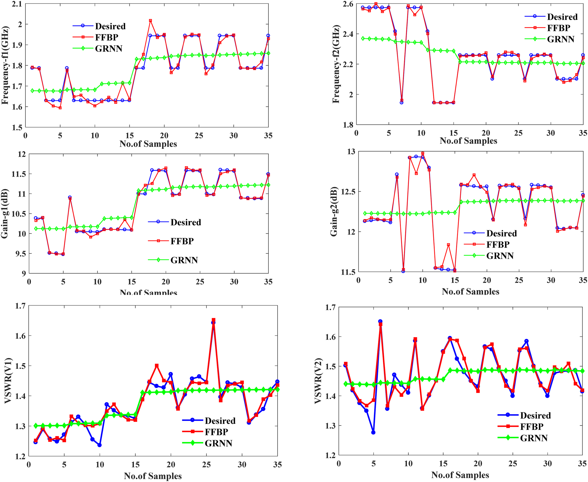
Fig. 12. Comparison of desired outputs with FFBP and GRNN for frequency, gain and VSWR.
From graphical results it has been analyzed that FFBP neural network outputs are near to desired output parameters as compared to GRNN outputs. So, it has been observed that FFBP neural network shows minimum error.
Comparison of proposed work with previous work
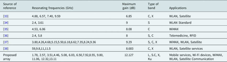
From the study of different research papers, it has been observed that various types of fractal antenna arrays are designed and simulated with Ansoft high frequency structure simulator (HFSS). A multiband response has been achieved for designed array. The value of gain has observed at each resonating frequency. Arrays presented in references [Reference Sagne, Batra and Zade33–Reference Viswason and Santosh Kumar38] work at the most 10 resonating frequencies with maximum gain of 9.29 dB and used in wireless and biomedical fields but the proposed array works at 13 frequencies with maximum gain of 12.127 dB and can be used in L, S, C, X and Ku band applications. Thus, the proposed array is better than the arrays present in literature. A comparison of proposed work with existing work has been shown in Table 3.
Table 3. Comparison of proposed work with existing work.
Conclusions
A fractal antenna array with circular-shaped elements has been designed with different substrate materials, substrate heights, radii, and simulated with HFSS software. In proposed fractal antenna array, the value of absolute error 0.01712 mm has been obtained for radius. A comparison of measured and neural outputs has been done which shows the value of absolute error −0.00700 GHz, 0.00702 GHz, −0.06038 dB, −0.00551 dB, −0.00657 and −0.01825 for frequency (f 1, f 2), gain (g 1, g 2) and VSWR (v 1, v 2) respectively for designed fractal antenna array. So, it is an effective approach for optimization of designing and output parameters of a fractal antenna array. The proposed array has also been compared with other existing fractal arrays and it is concluded that designed array has more gain than existing arrays presented in literature and can be used for L, S, C, X and Ku band applications.
 Er. Sunita Rani was born at Budhlada in Punjab. She received her B.Tech degree in electronics and instrumentation from Punjab Technical University Jalandhar. She also received her M.Tech degree in electronics and communication engineering from Yadavindra College of Engineering, Punjabi University Patiala. Currently she is pursuing her Ph.D. (part time) in antenna array from Punjabi University Patiala, Punjab, India. Currently, she is working as an assistant professor in the Electronics and Communication Engineering Department at Yadavindra College of Engineering Off-Campus of Punjabi University Patiala, Punjab, India. She has published more than 25 research papers in several International Journals and International and National Conferences. Her research interests lie in the field of Fractal Antenna Array, Neural Networks, Optimization techniques and Virtual Instrumentation. Er. Sunita is a member of the Institution of Engineers.
 Dr. Jagtar Singh Sivia born in Bathinda, Punjab in 1976. He received his B.Tech degree from Punjab Technical University, Jalandhar, Punjab in electrical and electronics communication engineering in 1999 and he had obtained his master's degree from Punjab Technical University, Jalandhar in 2005. He obtained his Ph.D. degree from Sant Longowal Institute of Engineering and Technology, Longowal, Punjab. Currently, he is a professor in Electronics and Communication Section at Yadavindra College of Engineering, Off-Campus of Punjabi University, Patiala, Punjab, India. He has published more than 75 papers in several International Journals and International and National Conferences. His main interests are in neural networks, electromagnetic waves, genetic algorithms, antenna system engineering. Dr. Sivia is a member of the Institution of Engineers in India, Indian Society of Technical Education and International Association of Engineers.