2. System description

Figure 1 shows the three-dimensional (3D) view of the 4-RR(SS)₂ four-DOF high-speed parallel robot mechanism. The mechanism mainly includes a static platform, a moving platform, and four branch chains connecting the static and moving platforms with the same structure. Each branch chain comprises a rotating fork, an active arm, and a follower arm containing a parallelogram. The type of the chain is RR(SS)₂, where R represents the rotating pair, R represents the active rotating pair, and (SS)₂ represents a parallelogram structure with a spherical joint at both ends. The branch chain with R(SS)₂ as the topological structure has a 3D translation. Thus, each branch chain is connected to the static platform by a rotating fork, that is, each branch chain is added with a rotating pair, which is why each branch chain has the ability of 3D translation and one-dimensional rotation. As the rotation axes of the rotation pairs added by the four branch chains are parallel to the vertical axis, the moving platform can three-dimensionally translate and rotate around the vertical axis. Notably, to provide the rotational torque around the vertical axis, the four branch chains are designed as offset structures and the movable platform is designed as a nonsquare structure. Owing to the single-action platform structure of the robot, the weight of moving parts can be effectively reduced, improving the dynamic characteristics of the robot and allowing high speed and acceleration. Compared with X4 parallel manipulator (which is a R(SS)₂R parallel manipulator) [Reference Xie and Liu24], the difference lies in the position setting of revolute pairs with axes parallel to each other. The proposed parallel manipulator may be able to further decrease the size of the moving platform since the revolute pairs are moved from being connected with the moving platform to being connected with the static platform. This is beneficial to improve the acceleration and deceleration performance of the mechanism.

Figure 1. Model of 4-RR(SS)2 high-speed parallel robot. 1. Static platform 2. Servo motor 3. Rotating fork. 4. Active arm 5. Follower arm 6. Moving platform.

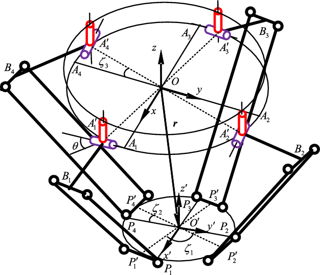
Figure 2. Schematic of the organization.

Figure 2 shows the structure of the mechanism. In Fig. 2, ${P'_{\!\!i}}$ and ${A'_{\!\!i}\;}$ ( $i = 1,2,3,4$ ) are the hinge centers connecting the branch chain $i$ and the moving and static platforms, respectively; ${B_i}$ is the hinge center connecting the active arm and the follower arm. Let ${A_i}$ and ${P_i}$ be the positions before the offset of the branches of ${A'_{\!\!i}}$ and ${P'_{\!\!i}}$ . A fixed reference coordinate system $O - xyz$ is established with the geometric center point of the stationary platform as the origin, where the x-axis direction points from point $O$ to point ${A_1}$ , $z \bot {A_1}{A_2}{A_3}{A_4}$ , and the y-axis satisfies the right-hand rule. In the initial position, the centerlines of the R turning pairs on ${A'_{\!\!3}}$ and ${A'_{\!\!1}}$ are still parallel to the y-axis after offset installation and the center lines of the R turning pairs on ${A'_{\!\!4}}$ and ${A'_{\!\!2}}$ are still parallel to the x-axis after offset installation. The geometric center point of the moving platform is considered as the origin to construct the moving platform conjoined coordinate system $O' - x'y'z'$ , where the x-axis direction points from point $O'$ to point ${P_1}$ , $z' \bot {P_1}{P_2}{P_3}{P_4}$ , and the y-axis satisfies the right-hand rule. For the convenience of description, here, ${\zeta _1}$ is the structural angle of the moving platform, that is, the obtuse angle between $\overline {{{P'}_{\!\!1}}{{P'}_{\!\!3}}} $ and $\overline {{{P'}_{\!\!2}}{{P'}_{\!\!4}}} $ , and ${\zeta _2}$ and ${\zeta _3}$ are the assembly offset angles of the moving and static platforms, respectively, that is, the acute angles between $\overline {{P_1}{P_3}} $ and $\overline {{{P'}_{\!\!1}}{{P'}_{\!\!3}}} $ and between $\overline {{A_1}{A_3}} $ and $\overline {{{A'}_{\!\!1}}{{A'}_{\!\!3}}} $ , respectively.

3. Kinematics modeling

As shown in Fig. 2, the position vector of the reference point $O'$ of the moving platform in the reference coordinate system $O - xyz$ can be expressed as

(1) \begin{align}{\textbf{r}} = {{\textbf{a}}_i} + {L_1}{{{\textbf{u}}}_i} + {L_2}{{{\textbf{w}}}_i} - {{{\textbf{p}}}_i},\quad\begin{array}{*{20}{c}}{} {i = 1,2,3,4}\end{array}\end{align}

where ${L_1}$ and ${L_2}$ are the rod lengths of the active arm and the follower arm, respectively, ${{{\textbf{u}}}_i}$ and ${{{\textbf{w}}}_i}$ are their unit direction vectors, and ${{{\textbf{a}}}_i}$ and ${{{\textbf{p}}}_i}$ are the position vectors from point $O$ to ${A'_{\!\!i}}$ and $O'$ to ${P'_{\!\!i}}$ , respectively. Furthermore, ${{{\textbf{a}}}_i} = {R_1}{\left( {\begin{array}{*{20}{c}}{\cos ({\gamma _i}{\rm{ + }}{\zeta _3})}{\sin ({\gamma _i}{\rm{ + }}{\zeta _3})}0\end{array}} \right)^{\rm{T}}}$ , ${{{\textbf{u}}}_i} = {\left( {\begin{array}{*{20}{c}}{\cos \left( {\theta + {\gamma _i}} \right)\cos {\alpha _i}}{\sin \left( {\theta + {\gamma _i}} \right)\cos {\alpha _i}}{ - \sin {\alpha _i}}\end{array}} \right)^{\rm{T}}}$ , ${\gamma _i} = \left( {i - 1} \right){\rm{\pi }}/2$ , ${{{\textbf{p}}}_i} = {R_2}{\left( {\begin{array}{*{20}{c}}{\cos {\beta _i}}{\sin {\beta _i}}0\end{array}} \right)^{\rm{T}}},\,\,{\beta _i} = \left( {i - 1 - {\varepsilon _i}} \right){\rm{\pi }}/2 + {\varepsilon _i}{\zeta _1} + {\zeta _2} + \theta ,\,\,{\varepsilon _i} = \left\{ {\begin{array}{*{20}{c}}{0,{\rm{ }}i = 1,3}\\{1,{\rm{ }}i = 2,4}\end{array}} \right.$ , ${R_1}$ and ${R_2}$ are the radii of the moving and static platform, respectively, ${\alpha _i}$ is the rotation angle of the active arm, and ${\gamma _i}$ is the azimuth angle of ${A_i}$ . $\theta $ is the rotation angle around the z-axis when the mechanism moves.

Combining Eq. (1) and 4-RR(SS)₂ mechanism characteristics can be obtained as

(2) \begin{align}{\alpha _i} = 2\arctan \frac{{{A_i} \pm \sqrt {{A_i}^2 + {B_i}^2 - {C_i}^2} }}{{{B_i}^2 - {C_i}^2}}\end{align}

(3) \begin{align}{{{\textbf{w}}}_i} = \frac{{{{\textbf{r}}} + {{{\textbf{p}}}_i} - {{{\textbf{a}}}_i} - {L_1}{{{\textbf{u}}}_i}}}{{{L_2}}}\end{align}

where ${A_i} = 2{L_1}{m_{iz}}$ , ${B_i} = - 2{L_i}{m_{ix}}\cos (\theta + {\gamma _i}) + 2{L_i}{m_{iy}}\sin (\theta + {\gamma _i})$ , and ${C_i} = {\left| {{m_i}} \right|^2} + {L_1}^2 - {L_2}^2$ ; $i = 1,2,3,4$ , $ \pm $ are determined according to the initial configuration of the mechanism:

Derivation of Eq. (1) leads to

(4) \begin{align}{\dot{{\textbf{r}}}} = {L_1}\left( {{{\boldsymbol{\omega }}_{1i}} \times {{{\textbf{u}}}_i}} \right) + {L_2}\left( {{{\boldsymbol{\omega }}_{2i}} \times {{{\textbf{w}}}_i}} \right) - \dot \theta {\hat{{\textbf{z}}}} \times {{{\textbf{p}}}_i}\end{align}

where ${\dot{{\textbf{r}}}}$ represents the linear velocity of point $O'$ of the moving platform. ${{\boldsymbol{\omega }}_{1i}}$ and ${{\boldsymbol{\omega }}_{2i}}$ represent the angular velocity of the active arm and the follower arm, respectively. $\dot \theta $ is the angular velocity of the rotating fork around the vertical axis, ${\hat{{\textbf{z}}}}$ is the z-axis unit direction vector, ${{\boldsymbol{\omega }}_{1i}} = \dot \theta {\hat{{\textbf{z}}}} + {\dot \alpha _i}{{{\textbf{v}}}_i}$ , ${\dot \alpha _i}$ is the angular velocity of the active arm relative to the rotating fork, ${{{\textbf{v}}}_i}$ is the unit vector of the axis, where the active R pair is located, which can be expressed as ${{{\textbf{v}}}_{\rm{i}}} = {\left( {\begin{array}{*{20}{c}}{ - \sin \left( {\theta + {\gamma _{\rm{i}}}} \right)}{\cos \left( {\theta + {\gamma _i}} \right)}0\end{array}} \right)^{\rm{T}}}$ . By multiplying both sides of Eq. (4) by ${{{\textbf{w}}}_i}$ and arranging them into a matrix form, we obtain

(5) \begin{align}{\dot{\boldsymbol \alpha }} = {{\textbf{J}}}{\dot{{\textbf{x}}}},\end{align}

\begin{align*}{\dot{\boldsymbol \alpha }} & = {\left( {{{\dot \alpha }_1}{\rm{ }}{{\dot \alpha }_2}{\rm{ }}{{\dot \alpha }_3}{\rm{ }}{{\dot \alpha }_4}} \right)^{\rm{T}}},\\ {\dot{{\textbf{x}}}} & = {\left( {{{{\dot{{\textbf{r}}}}}^{\rm{T}}}{\rm{ }}\dot \theta } \right)^{\rm{T}}},\,\,{{\textbf{J}}} = {{\textbf{J}}}_q^{ - 1}{{{\textbf{J}}}_x},\,\,{{\textbf{J}}}_q^{} = {\rm{diag}}\left( {{L_1}{{\textbf{w}}}_i^{\rm{T}}\left( {{{{\textbf{v}}}_i} \times {{{\textbf{u}}}_i}} \right)} \right),\,\,{J_x} = \left[ {\begin{array}{*{20}{c@{\quad}c}}{\textbf{w}^{T}_{1}}& {\textbf{w}^{T}_{1}(\hat{\textbf{z}}\times(L_{1}\textbf{u}_{1}-\textbf{p}_{1}))}\\ {\textbf{w}^{T}_{2}}& {\textbf{w}^{T}_{2}(\hat{\textbf{z}}\times(L_{1}\textbf{u}_{2}-\textbf{p}_{2}))} \\ {\textbf{w}^{T}_{2}}& {\textbf{w}^{T}_{3}(\hat{\textbf{z}}\times(L_{1}\textbf{u}_{3}-\textbf{p}_{3}))} \\ {\textbf{w}^{T}_{4}}& {\textbf{w}^{T}_{4}(\hat{\textbf{z}}\times(L_{1}\textbf{u}_{4}-\textbf{p}_{4}))} \end{array}} \right]\end{align*}

where ${{\textbf{J}}}_q^{}$ and ${{\textbf{J}}}_x^{}$ represent the direct and indirect Jacobian matrix, respectively, and ${{\textbf{J}}}$ represents the Jacobian matrix, which represents the mapping relationship between the end speed and that of the active joint.

Taking the derivative of Eq. (4) gives

(6) \begin{align}{\ddot{{\textbf{r}}}} = {L_1}{{\dot{\boldsymbol \omega }}_{1i}} \times {{{\textbf{u}}}_i} + {L_1}{{\boldsymbol{\omega }}_{1i}} \times {\rm{(}}{{\boldsymbol{\omega }}_{1i}} \times {{{\textbf{u}}}_1}{\rm{)}} + {L_2}{{\dot{\boldsymbol \omega }}_{2i}} \times {{{\textbf{w}}}_i} + {L_2}{{\boldsymbol{\omega }}_{2i}} \times ({{\boldsymbol{\omega }}_{2i}} \times {{{\textbf{w}}}_i}) - \left[ {{\dot{\boldsymbol \omega }} \times {{{\textbf{p}}}_i} + {\boldsymbol{\omega }} \times {\rm{(}}{\boldsymbol{\omega }} \times {{{\textbf{p}}}_i}{\rm{)}}} \right].\end{align}

Substituting the derivative of ${{\boldsymbol{\omega }}_{1i}}$ and ${\boldsymbol{\omega }}$ into Eq. (6), then taking the dot product on both sides of Eq. (6) with ${{{\textbf{w}}}_i}$ , and arranging them into a matrix form yields

(7) \begin{align}{\ddot{\boldsymbol \alpha }} = {{\textbf{J}}}{\ddot{{\textbf{x}}}} + f({\dot{{\textbf{x}}}}),\end{align}

where ${\ddot{\boldsymbol \alpha }} = {({\ddot \alpha _1}{\rm{ }}{\ddot \alpha _2}{\rm{ }}{\ddot \alpha _3}{\rm{ }}{\ddot \alpha _4})^{\rm{T}}}$ , ${\ddot{{\textbf{x}}}} = {({{\ddot{{\textbf{r}}}}^{\rm{T}}}{\rm{ }}\ddot \theta )^{\rm{T}}}$ , ${{\textbf{f}}} = {({f_1}{\rm{ }}{f_2}{\rm{ }}{f_3}{\rm{ }}{f_4})^{\rm{T}}}$ , ${f_i} = {{\dot{{\textbf{x}}}}^{\rm{T}}}{{{\textbf{H}}}_i}{\dot{{\textbf{x}}}}/{L_1}^2$ , ${{{\textbf{H}}}_i} = {U_i}\left( {{{{\textbf{Q}}}_i}{\rm{ + }}{L_1}{{{\textbf{w}}}_i} \cdot {{{\textbf{u}}}_i}{{{\textbf{J}}}_{{\boldsymbol{\omega }}1i}}^{\rm{T}}{{{\textbf{J}}}_{{\boldsymbol{\omega }}1i}}{\rm{ + }}\frac{1}{{{L_2}}}{{{\textbf{J}}}_{{\boldsymbol{\omega }}2i}}^{\rm{T}}{{{\textbf{J}}}_{{\boldsymbol{\omega }}2i}}} \right)$ , ${U_i} = \dfrac{{{L_1}}}{{{{{\textbf{w}}}_i} \cdot [{{{\textbf{v}}}_i} \times {{{\textbf{u}}}_i}]}}$ , $\begin{array}{*{20}{c}}{{{{\textbf{J}}}_{\omega 1i}}}\end{array}{\rm{ = (}}{\hat{{\textbf{z}}}}\left[ {\begin{array}{*{20}{c}}0001\end{array}{\rm{ }}} \right]{\rm{ + }}{{{\textbf{v}}}_i}{{{\textbf{J}}}_i}{\rm{)}}$ , and $\begin{array}{*{20}{c}}{{{{\textbf{J}}}_{\omega 2i}}}\end{array}{\rm{ \;=\; }}\frac{1}{{{L_2}}}\left[ {{{{\textbf{w}}}_i} \times } \right]\left( {[{E_3}{\rm{ }}\left( {{L_1}{{{\textbf{u}}}_i} - {{{\textbf{p}}}_i}} \right) \times {\hat{{\textbf{z}}}}] - {L_1}\left( {{{{\textbf{v}}}_i} \times {{{\textbf{u}}}_i}} \right){{{\textbf{J}}}_i}} \right)$ ${{{\textbf{Q}}}_i}{\rm{ \;=\; }}\left[ {\begin{array}{*{20}{c@{\quad}c@{\quad}c@{\quad}c}}0& 0& 0 &{{L_1}{{{\textbf{J}}}_{i1}}{{{\dot{{\textbf{v}}'}}}_i} \cdot [{{{\textbf{w}}}_i} \times {{{\textbf{u}}}_i}]}\\0& 0& 0 &{{L_1}{{{\textbf{J}}}_{i2}}{{{\dot{{\textbf{v}}'}}}_i} \cdot [{{{\textbf{w}}}_i} \times {{{\textbf{u}}}_i}]}\\0& 0 &0& {{L_1}{{{\textbf{J}}}_{i3}}{{{\dot{{\textbf{v}}'}}}_i} \cdot [{{{\textbf{w}}}_i} \times {{{\textbf{u}}}_i}]}\\0 &0& 0 &{{L_1}{{{\textbf{J}}}_{i4}}{{{\dot{{\textbf{v}}'}}}_i} \cdot [{{{\textbf{w}}}_i} \times {{{\textbf{u}}}_i}] - {{{\textbf{w}}}_i} \cdot {{{\textbf{p}}}_i}}\end{array}{\rm{ }}} \right]$ , where ${{{\textbf{J}}}_i}$ represents the row vector of the $i$ th row of ${{\textbf{J}}}$ .

4. Motion law optimization

From the cam design theory, common motion laws include sinusoidal acceleration, modified trapezoidal acceleration, and 3-4-5 polynomials [Reference Zhang25]. To obtain the optimal motion law suitable for the 4-RR(SS)₂ parallel mechanism, the above-mentioned three motion laws are compared and analyzed. The variation law of 3-4-5 polynomial acceleration ${a_{345}}$ , sinusoidal acceleration ${a_{\sin }}$ , and modified trapezoidal acceleration ${a_{MT}}$ with time t can be expressed as follows:

(8) \begin{align}{a_{345}}(t) = \frac{{{a_{\max }}}}{{5.7735}}\left[ {60\left( {\frac{t}{{{T_{345}}}}} \right) - 180{{\left( {\frac{t}{{{T_{345}}}}} \right)}^2} + 120{{\left( {\frac{t}{{{T_{345}}}}} \right)}^3}} \right],\end{align}

(9) \begin{align}{a_{\sin }}\left( t \right) = {a_{\max }}\sin \left( {\frac{{2\pi }}{{{T_{\sin }}}} \cdot t} \right),\end{align}

(10) \begin{align}{a_{MT}}(t){\rm{ \;=\; }}\left\{ {\begin{array}{*{20}{ll}}{{a_{\max }}\sin (4\pi t/{T_{MT}})} & {(0 \le t \le 0.125{T_{MT}})}\\{{a_{\max }}{\rm{ }}} & {(0.125{T_{MT}} \lt t \le 0.375{T_{MT}})}\\{{a_{\max }}\cos \left[ {4\pi (t - 0.375{T_{MT}})/{T_{MT}}} \right]{\rm{ }}} & {(0.375{T_{MT}} \lt t \le 0.625{T_{MT}})}\\{ - {a_{\max }}{\rm{ }}} & {(0.625{T_{MT}} \lt t \le 0.875{T_{MT}})}\\{ - {a_{\max }}\cos \left[ {4\pi (t - 0.875{T_{MT}})/{T_{MT}}} \right]{\rm{ }}} & {(0.875{T_{MT}} \lt t \le {T_{MT}})}\end{array}} \right.\!\!,\end{align}

where ${a_{\max }}$ represents the maximum acceleration and ${T_{345}}$ , ${T_{\sin }}$ , and ${T_{MT}}$ are the periods of the three laws of motion. S is defined as the total length of the motion path, and the periods of the three motion laws can be calculated as follows:

(11) \begin{align}{T_{345}} = \sqrt {\frac{{5.7735S}}{{{a_{\max }}}}} {\rm{ }}{T_{\sin }} = \sqrt {\frac{{2\pi S}}{{{a_{\max }}}}} {\rm{ }}{T_{MT}} = \sqrt {\frac{{4.889S}}{{{a_{\max }}}}} \end{align}

The selection criterion of the movement law is whether the movement is fast and stable. It can be assessed by comparing the movement period T, acceleration peak a _max, and jump peak j _max under the same path S. The smaller the a _max and j _max, the more stable is the movement of the mechanism. The formula of the index j _max is as follows:

(12) \begin{align}{j_{\max }} = {C_j}S\frac{1}{{{T^3}}}\end{align}

where C _j is the characteristic coefficient. The characteristic coefficients C _j of the 3-4-5 polynomial, sine acceleration, and modified trapezoidal acceleration are 60, 39.5, and 61.4, respectively.

The typical pick-and-place operation path of a high-speed parallel robot is the Adept gate-shaped trajectory, as shown in Fig. 3, where the AB and CD sections represent the vertical motions and the BC section represents the horizontal motions. Without loss of generality, segments AB and BC are considered motion trajectories to optimize the above-mentioned three motion laws. In this case, the acceleration peak value a _max is set to 50 m/s², the vertical displacement of section AB is 0.025 m, and the horizontal displacement of section BC is 0.30 m.

Figure 3. Adept door-shaped trajectory.

Tables I and II show the peak value and time of jump at the end reference point and active arm joint, respectively, when the end trajectory is segment AB. Tables III and IV show the peak value and time of jump at the end reference point and active arm joint when the end trajectory is the BC segment, respectively.

Under the same terminal acceleration peak condition, irrespective of whether the mechanism performs a horizontal or vertical movement, the modified trapezoidal movement law takes the shortest time. Therefore, in the pursuit of high-speed parallel mechanism trajectory-planning research, the modified trapezoidal motion law can be used to achieve the highest frequency motion. At the same time, when the modified trapezoidal motion law is adopted, the peak value of the jerk at the end reference point is 2.26 times that of the sine function and 1.31 times that of the 3-4-5 degree polynomial. For the active arm, the peak angular acceleration of the modified trapezoidal motion law is also the highest, implying that the motion is unstable. Although the sine function motion law can minimize the peak value of the jump, the motion efficiency is also the lowest. Therefore, considering the length and stability of the motion, the 3-4-5 degree polynomial is selected as the motion law of the end trajectory of the mechanism.

5. Motion path planning

5.1. Gate-shaped trajectory

A typical Adept gate-shaped trajectory model comprises three straight lines, as shown in Fig. 3, where the lifting height h _d = 25 mm and the horizontal movement distance l _d = 300 mm. If the 3-4-5 polynomial motion law is applied to the entire gate-shaped trajectory path, the total length of the path is

(13) \begin{align}{S_d}{\rm{ \;=\; }}2{h_d} + {l_d},\end{align}

As shown in Fig. 4, assuming that the peak acceleration ${a_{\max }}$ of the 4-RR(SS)₂ parallel mechanism running along the Adept gate-shaped trajectory is 50 m/s², the angle, angular velocity, and angular acceleration changes of the four active arms of the mechanism can be obtained using the inverse solution model.

Figure 4 shows that when the end of the mechanism runs along the Adept gate-shaped trajectory, the angular accelerations of the four active arms experience abrupt changes in the orthogonal turning point. The rapid changes in the active joints during high-speed movement will have a greater impact on the mechanism. If stopping and restarting at right angles for stability causes the motion cycle to increase considerably, considering the Adept gate-shaped trajectory, the Lamé curve is used to transition the right-angled part.

Table I. Simulation results of extremity motion parameters in a vertical trajectory.

Table II. Simulation results of active arm-motion parameters during vertical trajectory.

Table III. Simulation results of terminal motion parameters in a horizontal trajectory.

Table IV. Simulation results of active arm-motion parameters in a horizontal trajectory.

Figure 4. Changes in the angle, angular velocity, and angular acceleration of the driving arm in the adept gate path (1, 2, 3, and 4 represent the label of the driving arm).

Figure 5. Lamé curve.

Figure 6. Adept gate-shaped trajectory after Lamé curve transition.

5.2. Lamé trajectory

Circular arc transition is a traditional approach of transitioning right-angled parts; however, often because of an abrupt change in curvature at the intersection of the straight line and circular arc, it causes a sudden centripetal acceleration, shaking the end-moving platform. A Lamé curve is also called a super elliptic curve because it exhibits curvature continuity, which is why it can avoid the impact of centripetal acceleration caused by sudden curvature in the trajectory.

As shown in Fig. 5, the Lamé curve is analyzed in the first quadrant, and its trajectory satisfies Eq. (14):

(14) \begin{align}{\left( {\frac{{\rm{u}}}{d}} \right)^3}{\rm{ + }}{\left( {\frac{{\rm{v}}}{e}} \right)^3}{\rm{ \;=\; }}1,\end{align}

where d is the long axis length and e is the short axis length.

To calculate the new trajectory length, the length of the Lamé curve $\widehat{APB}$ needs to be calculated first. In the coordinate system O-uv, the coordinate of point P can be expressed as

(15) \begin{align}{\rm{u}}\left( {{\omega _l}} \right) = \frac{d}{{{{\left( {1 + {{\left( {\frac{d}{e}\tan \left( {{\omega _l}} \right)} \right)}^3}} \right)}^{\frac{1}{3}}}}}\quad {\rm{ v}}\left( {{\omega _l}} \right) = \frac{{d\tan \left( {{\omega _l}} \right)}}{{{{\left( {1 + {{\left( {\frac{d}{e}\tan \left( {{\omega _l}} \right)} \right)}^3}} \right)}^{\frac{1}{3}}}}},\end{align}

where ${\omega _l}$ represents the angle between $\widehat{OP}$ and ${U}$ axis, ${\beta _l}$ represents the cut angle.

According to the arc length formula, $\widehat{AP}$ is expressed as

(16) \begin{align}AP = \int_0^{{\omega _l}}\! {{{\left\{ {{{\!\left[\! {{{\left( \!{{{d\left( {{{\tan }^2}{\omega _l} + 1} \right)} \over {{{\left( {{{\left( {{\dfrac{d}{e}}\tan {\omega _l}} \right)}^3} + 1} \right)}^{{1 \over 3}}}}}} \right)}^2} \!- {{{d^4}{{\tan }^3}{\omega _l}\left( {{{\tan }^2}{\omega _l} + 1} \right)} \over {{e^3}{{\left( {{{\left( {{\dfrac{d}{e}}\tan {\omega _l}} \right)}^3} + 1} \right)}^{{4 \over 3}}}}}} \right]}^2} + {{{d^8}{{\tan }^4}{\omega _l}{{\left( {{{\tan }^2}{\omega _l} + 1} \right)}^2}} \over {{e^6}{{\left( {{{\left( {{\dfrac{d}{e}}\tan {\omega _l}} \right)}^3} + 1} \right)}^{{8 \over 3}}}}}} \right\}}^{{1 \over 2}}}} d{\omega _l},\end{align}

As shown in Fig. 6, the length of the entire path can be obtained:

(17) \begin{align}{S_{Lame}}{\rm{ \;=\; }}2{h_d} + {l_d} - 2\left( {d + e} \right) + BC + DE,\end{align}

If the total length of the path is known, the total time T through the entire path can be obtained from Eq. (11). Furthermore, the total length of the gate-shaped trajectory path after the Lamé curve transition depends on the size of the two parameters d and e of the Lamé curve. Figure 7 shows the change rule of the total time T with respect to d and e under the 3-4-5 polynomial motion rule. Figure 7 shows that when d and e are both 0, that is, when the Lamé curve transition is not used, the gate-shaped trajectory movement time T is the longest, which is 0.2009 s. The movement duration T decreases as d and e increase. When d and e are 150 and 25 mm, respectively, under the gate-shaped trajectory constraint, the total movement duration T is the shortest, that is, 0.1922 s. There is no straight part on the track at this time.

Figure 7. Relationship between total time T and curve parameters d and e.

5.3. Motion decomposition

As shown in Fig. 8, according to the 3-4-5 polynomial motion law, the given acceleration peak value, total path length, path length $s(t)$ , absolute speed $v(t)$ , and acceleration $a(t)$ traversed by the end of the mechanism at any $t$ time can be determined. Based on the arc length formula (20), the angle ${\omega _l}$ can be obtained using the inverse solution; then, the velocity $({v_{\rm{u}}},{v_{\rm{v}}})$ and acceleration $({a_{\rm{u}}},{a_{\rm{v}}})$ in the plane coordinate system O-uv can be obtained, and further, the velocity $({v_x},{v_{\rm{y}}},{v_z})$ and acceleration $({a_x},{a_{\rm{y}}},{a_z})$ in the space coordinate system O-xyz can be obtained by conversion. Owing to the change toward the motion direction, the five-segment route comprising $\overline {AB} $ , BC, $\overline {CD} $ , DE, and $\overline {EF} $ must be decomposed. Furthermore, because the motion solution of the linear part is relatively simple, it will not be explained.

Figure 8. Motion decomposition solution process.

Decomposing the motion on the curve in the coordinate system O-uv gives

(18) \begin{align}\begin{array}{l}\left\{ {\begin{array}{*{20}{c}}{{v_{\rm{u}}} = v\left( t \right)\cos {\beta _l}}\\{{v_{\rm{v}}} = v\left( t \right)\sin {\beta _l}}\end{array}} \right.\\[8pt] \left\{ {\begin{array}{*{20}{c}}{{a_{\rm{u}}} = a\left( t \right)\cos {\beta _l} - v\left( t \right)\sin {\beta _l}\frac{{d{\beta _l}}}{{dt}}}\\[4pt] {{a_{\rm{v}}} = a\left( t \right)\sin {\beta _l} + v\left( t \right)\cos {\beta _l}\frac{{d{\beta _l}}}{{dt}}}\end{array}} \right.,\end{array}\end{align}

where ${\beta _l}$ is the cut angle of the curve in Fig. 5, which can be expressed by the slope of the curve:

(19) \begin{align}\tan {\beta _l} = \frac{{d{\rm{v}}}}{{d{\rm{u}}}} = - \frac{e}{d}{\left( {\frac{{\rm{u}}}{d}} \right)^2}{\left[ {1 - {{\left( {\frac{{\rm{u}}}{d}} \right)}^3}} \right]^{ - \frac{2}{3}}},\end{align}

and $\frac{{d{\beta _l}}}{{dt}}$ can be obtained by deriving the two sides of Eq. (17):

(20) \begin{align}\frac{{d{\beta _l}}}{{dt}} = - {\cos ^2}{\beta _l}\left( {{V_1}} \right)\frac{{d{\rm{u}}}}{{dt}},\end{align}

where

(21) \begin{align}{V_1} = \frac{{2e{{\rm{u}}^4}}}{{{d^6}{{\left( {1 - {{\left( {\dfrac{{\rm{u}}}{d}} \right)}^3}} \right)}^{\frac{5}{3}}}}} + \frac{{2e{\rm{u}}}}{{{d^3}{{\left( {1 - {{\left( {\dfrac{{\rm{u}}}{d}} \right)}^3}} \right)}^{\frac{2}{3}}}}}.\end{align}

After the two-dimensional motion decomposition of the curve part is obtained, it can be converted into position $(x,y,z)$ , velocity $({v_x},{v_{\rm{y}}},{v_z})$ , and acceleration $({a_x},{a_{\rm{y}}},{a_z})$ in the O-xyz coordinate system as follows:

(22) \begin{align}\left\{ \begin{array}{l}x = \cos \theta ({\rm{u + }}{C_1})\\y = \sin \theta ({\rm{u + }}{C_1})\\z = {\rm{v + }}{C_2}\end{array} \right.{\rm{ }}\left\{ \begin{array}{l}{v_x} = \cos \theta {v_{\rm{u}}}\\{v_y} = \sin \theta {v_{\rm{u}}}\\{v_z} = {v_{\rm{v}}}\end{array} \right.{\rm{ }}\left\{ \begin{array}{l}{a_x} = \cos \theta {a_{\rm{u}}}\\{a_y} = \sin \theta {a_{\rm{u}}}\\{a_z} = {a_{\rm{v}}}\end{array} \right.\end{align}

In formula (22), ${C_1}$ and ${C_2}$ are determined by the size of the curve parameters and specific road section where the end is located.

Figure 9 shows the change in angle, angular velocity, and angular acceleration of the active arm over time when a _max = 50 m/s², d = 50 mm, and e = 10 mm. The figure shows that after the Lamé curve is used to transition the two right angles of the trajectory, compared with the traditional Adept gate-shaped trajectory, the uneven changes in the trajectory of the No. 1 and No. 3 active arm joints at the gate-shaped corners are improved.

Figure 9. Changes in the angle, angular velocity, and angular acceleration of the driving arm under the Lamé trajectory (d = 50 mm and e = 10 mm. 1, 2, 3, and 4 represent the active arm label).

In addition, to reveal the influence of the parameters d and e of the Lamé curve on the smoothness of motion, Fig. 10 shows the change law of the peak angular acceleration $\mathop {\max }\limits_i {\ddot \alpha _i}$ of all active arms with respect to d and e. Figure 10 shows that $\mathop {\max }\limits_i {\ddot \alpha _i}$ decreases with increase in d and e. When d has the maximum value of 150 mm (half of the gate-shaped trajectory length l _d) and e has the maximum value of 25 mm (the gate-shaped trajectory height h _d), the minimum value of $\mathop {\max }\limits_i {\ddot \alpha _i}$ is 2.983 × 10⁴ °/s². Therefore, to minimize the movement duration T and the acceleration peak $\mathop {\max }\limits_i {\ddot \alpha _i}$ , the maximum values for both d and e should be substituted, that is, d = 150 and e = 25 mm. The active arm angle, angular velocity, and angular acceleration change laws are shown in Fig. 11. The curve of the motion parameters is smoother, and the peak angular acceleration is reduced. Figure 12 shows the shape of the trajectory path.

Figure 10. Relationship between $\mathop {\max }\limits_i {\ddot \alpha _i}$ and curve parameters d and e.

Figure 11. Changes in the angle, angular velocity, and angular acceleration of the driving arm under the Lamé trajectory (d = 150 and e = 25 mm. 1, 2, 3, and 4 represent the active arm label).

Figure 12. Lamé curve path (d = 150 and e = 25 mm).

Figure 13. Block diagram of Lamé path interpolation.

Figure 14. Lamé angle function block and Lamé arc length function block.

6. Interpolated motion control

According to previous studies, the Lamé trajectory is less used because the complex arc length given by Eq. (20) must be used to solve the curve angle ${\omega _l}$ in reverse when its motion needs to be decomposed. This section solves this problem using numerical solution and deduplication optimization methods.

6.1. Interpolation point solution

The Lamé path interpolation program is shown in Fig. 13. First, input parameters such as d, e, and a _max are used to calculate the total path length S and the movement duration T and discretize them. Second, according to the selected motion law, the position of the mechanism on the curved track at the current moment of motion is calculated and verified. If it is in the horizontal or vertical position, it can be directly assigned. If it is in the curve position, the angle ${\omega _l}$ is obtained using the Lamé angle module and the motion decomposition is completed based on the calculation of the parameter equation. Finally, the position data in the 3D coordinate system O-xyz obtained after decomposition are subjected to inverse solution and deduplication processing and the interpolation position array of the rotation angle of the active arm can then be outputted.

The angle ${\omega _l}$ is calculated using the Lamé arc length function block and the Lamé angle function block, as shown in Fig. 14. The Lamé arc length function block discretizes π/2 with a step length of 0.001 and then calculates the arc-length array corresponding to different angles from 0 to π/2 using Eq. (17). The Lamé angle function block searches and compares the input total path length ls at a certain moment with the arc-length array calculated using the arc length module to obtain the arc length closest to the path length ls and calculates the corresponding angle accordingly.

Figure 15. Occurrence of duplicate points.

Figure 16. Program block diagram of interpolation point deduplication.

6.2. Deduplication optimization

As shown in Fig. 15, the numerical solution method described above often has duplicate points in the results. As the speed of the parallel robot is extremely slow at the start of the movement, the distance traveled by the mechanism in the first few discrete 1-ms time intervals (ls1 and ls2 in the figure) is frequently smaller than the discrete angular step of the Lamé curve in the program (such as π/1000). At this time, multiple interpolation points appear in the arc corresponding to the unit discrete angle step. Therefore, the Lamé angle function block will repeatedly identify these interpolation points as the same angle when searching and comparing, resulting in duplicate points in the subsequent solving.

Figure 17. Interpolation point comparison before and after deduplication.

Figure 18. Experimental prototype.

When duplicate points exist in the interpolation point data, the theoretical speed calculated based on the position signal will be inconsistent with the actual speed; the actual speed is always zero at the duplicate point so that the unit discrete angle that was originally set to be completed by multiple interpolation cycles is directly completed only in the last cycle at several times the original speed. Finally, it results in an abrupt change in speed, causing the motor to run unstably and even jitter.

In this case, a part of the duplicate points can be removed by adjusting the difference between the angular and time discrete accuracy; however, this considerably increases the computational burden of the program and does not eliminate the duplicated points.

To completely prevent such situations, an additional function block of interpolation point deduplication is programmed by changing the difference in discrete accuracy, as shown in Fig. 16. After inputting an array with repeated points at the interpolation position, whether the adjacent points of the array are the same is assessed bit by bit. If they are the same, the repeat point counter is incremented and shifted to the next bit to continue the assessment. If the adjacent points are different, the scanning stops. At this time, the value of the duplicate point counter is the step length of the duplicate array segment. Afterward, the identified duplicate array segments are reassigned. Figure 17 shows that after the new assignment, the array segment increases or decreases at a constant speed, eliminating the abrupt change in speed and obtaining an array without duplicate points.

7. Experiment

A prototype of the robot is now used to verify the effectiveness of the aforementioned motion trajectory planning and interpolation motion control. Figure 18 shows the test prototype. The control system is TwinCAT 2 from Beckhoff.

Table V. Pick-and-place performance experiment (0° direction).

Table VI. Pick-and-place performance experiment (45° direction).

In this section, two representative motion directions of 0° and 45° are selected and the robot is allowed to run along the Lamé gate-shaped trajectory with different peak accelerations in the two directions. Simultaneously, the position error (PE), position-to-position velocity command (PTPVCMD), and actual current (IQ) of the motor are recorded during operation to reflect the performance of the mechanism. Referring to the task settings of the ABB Flexpicker manipulator, the round trip is recorded as a pick-and-place operation. The dwell time of the robot during the pick-and-place process is 0.035 s, and then, the pick-and-place frequency per minute can be calculated. The peak acceleration at the end is set to start from 10 m/s², and it gradually increases by 5 m/s² to test the pick-and-place frequency and performance of the robot prototype running on the Lamé trajectory.

As shown in Table V, when the robot is running in the 0° direction and the end acceleration is less than 35 m/s², the motor PE is minute and the command speed is also lower than the specified limit. When the end acceleration reaches 35 m/s², the pick-and-place frequency is 125 times/min and the command speed is 4034 r/min, which is close to the maximum motor speed of 5000 r/min. The motor current reaches the current limit value of 3.5 A set by ServoStudio, and its PE exceeds 0.1 r. At this time, increasing the acceleration will cause the driver’s power to be insufficient relative to the load and alarm.

As shown in Table VI, compared with the situation when the robot is running in the 0° direction, when the robot is running in the 45° direction, its command speed and current value are reduced. This is because the robot is mainly powered by only two motors in the 0° direction, and the corresponding active arm has a larger motion range; therefore, the speed will be greater. However, when the robot runs in the 45° direction, the four motors move in the same way and provide power evenly so that the motor speed and current are much smaller and higher command speeds can be achieved, thereby increasing the pick-and-place frequency. When the end acceleration is less than 50 m/s², the PE is minute, the command speed is also lower than the limit value, and the movement is extremely stable. When the end acceleration reaches 50 m/s², the pick-and-play frequency is 147 times/min. At this time, although the motor current has reached the set current limit value of 3.5 A and its PE has exceeded 0.1 r, its command speed is only 3752 r/min, which is even lower than that when the robot is running in the 0° direction at 35 m/s².

The test results show that the prototype adopts the optimized Lamé trajectory-planning method, which can achieve a stable pick-and-place frequency of up to 147 times/min, it is at a level similar to delta and Cross-IV robot [Reference Liu26]. Compared with previous experiments [Reference Song27], under the same end acceleration, the work efficiency of the traditional Adept gate-shaped trajectory-planning method is improved by 54.7%, and the work efficiency of the arc transition trajectory-planning method is improved by 34.8%. These results verify that the Lamé trajectory-planning method can greatly improve the work efficiency of the mechanism.