


1. Introduction
Recent advances in the ability to collect and categorize large amounts of linguistic data provide new opportunities for understanding the mechanisms of language variation and shift (Boas, Reference Boas, Austin, Aristar-Dry and Wittenburg2002; Zanuttini & Horn, Reference Zanuttini and Horn2014; Wood et al, Reference Wood, Horn, Zanuttini and Lindemann2015). Investigation into Texas German, an endangered but geographically widespread heritage language, is particularly useful for the investigation of koinéization, the process by which related dialects brought together into a new area mix together to create a new stable and homogenous variety. A koiné is a language contact phenomenon, a “stabilized contact variety which results from the mixing and subsequent leveling of features of varieties which are similar enough to be mutually intelligible, such as regional or social dialects” (Siegel, Reference Siegel2001:175). Sophisticated analysis of the variation and distribution of Texas German has been made possible by the ongoing Texas German Dialect Project (Boas et al, Reference Boas, Pierce, Weilbacher, Roesch and Halder2010). Boas (Reference Boas2009) utilizes Trudgill’s (Reference Trudgill2004) model of new dialect formation to argue that the presence of substantial variation in modern Texas German suggests that the koinéization process is incomplete. Alternatively, it could be understood as stable variation of a coherent unary dialect. To distinguish between these hypotheses, it is necessary to carefully examine the factors that are associated with this variation.
The focus of the current investigation is the variant pronunciation of sibilants in rst-clusters, which are pronounced as [s] in Standard German and either [s] or [∫] in Texas German. I examine the pronunciation of Wurst ‘sausage,’ Donnerstag ‘Thursday,’ and Haarbürste ‘hairbrush’ in the archives of the Texas German Dialect Project.
The goal of the current study is twofold. First, I supplement our knowledge of the wider pattern of variation with data from interviews collected by the TGDP throughout Texas. This will allow for a comparison between the previously studied pattern of the New Braunfels settlement with other communities to explore the extent to which the New Braunfels pattern is representative of Texas German as a whole. Secondly, I explore in more detail the patterns of variation found in modern Texas German by looking at social factors that could correlate with the expression of the variant: age, gender, and place of birth. I run a statistical clustering analysis on the geographical regions to answer the question of whether or not communities differ significantly in the expression of this variation, and the consequences this has for the development of a new world dialect.
I argue that the lack of a positive correlation for these factors, particularly for geographic region, provides evidence for the homogeneity of this feature. This paper is a case study of one particular phonological alternation found in Texas German, and therefore I cannot here make any definitive claims about the larger pattern of Texas German koiné formation. Rather, this study represents an important step in characterization of the variation that exists within Texas German as a whole.
The next section provides more background on the history and development of Texas German and an overview of previous scholarship on the region. This is followed by a discussion of Trudgill’s model of dialect formation as it relates to Texas German, and variation and dialect convergence more broadly, before an analysis of the data collected from the Texas German Dialect Project.
2. Texas German History and Development
Map 1, which depicts the reported birthplaces of every Texas German Dialect Project respondent as of 2017, provides a good picture of the overall spread of German settlement in Texas.

Map 1. TGDP respondent birthplaces
The map was created with ESRI’s Geographic Information Systems (GIS) software, ArcGIS.Footnote 1 Each token in the dataset is associated with the geographical coordinates of a speaker’s birthplace. These have been plotted on a map of Texas counties and major cities created from US Census data.
Large-scale German immigration to Texas began in the 1840s and continued until around 1890 (Biesele, Reference Biesele1930; Jordan, Reference Jordan1977:2). The earliest immigrations were to settled land in the eastern part of the Texas German belt. Settlers came primarily from the Low German areas of present-day north-central and northwestern Germany, particularly the Münsterland, Holstein, Mecklenburg, and Oldenburg (Jordan, Reference Jordan1966:63). Western settlement onto the Texas frontier began in the mid-1840s. Settlers came primarily from the Mid- and High German areas of present-day central Germany, particularly the Hessen-Nassau region, southern Hannover, Württemberg, and Alsace (Jordan, Reference Jordan1966:120), and established the major settlements Fredericksburg and New Braunfels. Compared to the eastern settlements, the settlements in the west were more isolated from the settlements of English-speaking Anglo-American settlers.
By 1890, there were roughly 145,000 German-Americans in the state, representing more than 6% of the state’s population (Jordan, Reference Jordan1977:2). Due to the general isolation of German-speaking communities along the Western frontier, a robust enclave of German speakers persisted well into the 20th century (Boas, Reference Boas2009:47).
Despite the advent of English-only education laws in the 1890s that were relatively unenforced, the German belt represented a robust linguistic enclave, or Sprachinsel, until World War I. German was the language of education, the press, religion, and commerce. This situation shifted dramatically between World War I and II due to increased mobility and the stigma of the German language. In almost all cases, children born after World War II were raised entirely in English. While Texas German may have as many as 6,000 modern-day speakers, almost all of them are over the age of seventy (Salmons, Reference Salmons1983; Wells, Reference Wells1985; Boas, Reference Boas2009:74).
Much of the research on Texas German in the 20th century focused on a variety of German spoken in single settlements (Eikel Reference Eikel1949, Reference Eikel1966a, Reference Eikel1966b, Reference Eikel1967; Clardy, Reference Clardy1954; Gilbert, Reference Gilbert1965). The settlement of New Braunfels in Comal County was the research site for Eikel (Reference Eikel1954) and Gilbert (Reference Gilbert1963), while Wilson (Reference Wilson1960) focuses on the German of Lee and Fayette Counties, and Guion (Reference Guion, Sture Ureland and Clarkson1996) looks at the settlement of Fredericksburg and surrounding Gillespie County. The noteworthy exception to this pattern is Gilbert (Reference Gilbert1972), presenting an extensive linguistic atlas of Texas German compiled through interviews with 286 informants throughout Texas. The atlas maps the geographical distribution of various phonological, morphological, and syntactic features which vary in Texas German.
Boas (Reference Boas2009) is a study of Texas German based on the earliest interviews conducted by the Texas German Dialect Project (TGDP), a central database of Texas German interviews at the University of Texas. The data from Boas (Reference Boas2009) comes from the settlement of New Braunfels and surrounding Comal County; the German of this community has been relatively homogenous, allowing a comparison of Boas’ results with the results of other studies from the previous century (Boas, Reference Boas2009:16). Boas (Reference Boas2009) is based on the interviews from 52 speakers around New Braunfels, using open interviews and samples of the same questionnaires used by Gilbert (Reference Gilbert1972).
Boas corroborates the presence of variant features found in Gilbert (Reference Gilbert1972) for present-day Texas German. Although Gilbert maps extensive variation in Texas German, he conceives of Texas German as a whole: “The trend is clearly toward a dissolution of the old, fragmented, mutually unintelligible (or at best partially intelligible) dialects, either by outright replacement or by gradual modification to form a new type of speech, which, although far from uniform, enjoys sufficient common characteristics to merit the generic name, Texas German.” (Gilbert Reference Gilbert1972:4). Boas, conversely, concludes that the process of new dialect formation was incomplete when it was interrupted in the middle of the 20th century. The presence of continued inter- and intraspeaker variability indicates that the speech has not converged: “we find a broad spectrum of dialectal mixtures with considerable English admixture. What has traditionally been called ‘Texas German’ should thus be regarded as a collection of various subvarieties that share a limited set of linguistic features” (Boas, Reference Boas2009:98).
These two viewpoints represent different hypotheses about the nature of the variety (or varieties) of German spoken in Central Texas. The extent to which variation can be taken as evidence for the non-convergence of a group of dialects into a koiné will depend upon the precise nature of the variation and the model used to describe how a group of dialects converge to form a new dialect.
2.1 Variation in Texas German
Boas’ (Reference Boas2009) analysis of new dialect formation in Texas German is based on Trudgill’s (Reference Trudgill2004) model, which describes how a dialect mixture will cohere into a new dialect. This occurs over the course of three stages which correspond roughly to generations of settlement in a homogenous community without a previously established language population. Trudgill’s model is deterministic and predicts the survival of dialectal variants based on strict proportionality at the feature level.
The first stage of Trudgill’s model consists of rudimentary leveling and interdialect development of the adult immigrant generation. Accommodation between adults begins en route to the destination, as the most salient features of traditional dialects are leveled in favor of intermediate forms. The second stage is characterized by extreme intra-individual and inter-individual variability of forms in the first native-born generation. Minority variant forms that exist below a certain rate are leveled out because they are so rare as to be unnoticed by young speakers. Children are exposed to a wide degree of variation in the environment. During the third and final stage, a focused, stable, and coherent dialect emerges. The majority variant in the original dialect mixture will survive in the new dialect. Table 1, adapted from Boas (Reference Boas2009:109), shows the successful leveling of a particular variant among Eikel’s 24 New Braunfels German speakers: rounded/unrounded front vowels ([y:]/[i:] and [ø]/[e:]).
Table 1. Age-graded Distribution of Rounded and Unrounded Front Vowels

Of the nine phonological features described by Boas, three appear to have gone through all three stages and exhibit little variation in the modern language. Other morphological and phonological features described by Boas (Reference Boas2009) show at least some evidence of leveling in the direction of one particular variant (Boas et al, Reference Boas, Ewing, Moran and Thompson2004; Pierce et al, Reference Pierce, Boas, Roesch, Bondi and Salmons2015). However, there is still substantial variation in the modern language. This includes the variant pronunciation of rst-clusters discussed in the next section. Boas takes this variation as evidence that the process of focusing was never completed: some features reached Stage Three, leaving only one surviving variant, while other features never left Stage Two.
The argument against convergence is that the koinéization process was interrupted by large-scale language shift to English, and variation in the modern language reflects this lack of convergence. There were at least three generations of Texas Germans before this shift began, so the process could conceivably have been completed in this timeframe. Kerswill (Reference Kerswill, Chambers, Trudgill and Schilling-Estes2002) notes that koinéization “typically takes two or three generations to complete, although it is achievable within one.” However, Kerswill and Trudgill (Reference Kerswill, Trudgill, Auer, Hinskens and Kerswill2005) present case studies for which koinéization has not occurred over multiple generations, typically due to sociological factors such as isolation and continuing in- and out-migration, although there are a finite number of these factors. Trudgill (Reference Trudgill2011) argues for two factors in particular that determine the speed of linguistic change: relative degree of isolation and relative social stability of the community. Focusing happens more quickly in isolated, socially homogenous communities. Baxter, Croft, and McKane (Reference Baxter, Blythe, Croft and McKane2009) criticize Trudgill’s (Reference Trudgill2004) model on the basis that solely deterministic processes cannot account for the emergence of a new dialect in an appropriate timeframe. They conclude that social and other non-deterministic factors must also be involved in order for the convergence to happen in a realistic timeframe.
For Texas German, these factors may include influence from surrounding English speakers and the influence of Standard German through media and education. Both of these factors are discussed by Boas, although he argues that the influence of Standard German on Texas German is overstated (contra Salmons & Lucht, Reference Salmons, Lucht, Thornburg-Panther and Fuller2006). Boas (Reference Boas2009) argues that the loss of the dative case is due to the leveling process of dialect contact rather than influence from English. Another factor is the continuing immigration from Germany during the latter half of the 19th century, and, to a lesser degree, the 20th. Nützel and Salmons (Reference Nützel and Salmons2011) note that ongoing immigration may be a factor in slowing the process of koinéization.
Trudgill’s model describes the process by which variant features in the dialect mixture come to stabilize such that a single variant prevails. This question of dialect convergence has recently been taken up by others working on Germanic heritage varieties in the United States (Johanneson & Salmons, Reference Johannessen and Salmons2015). The presence of significant intra- and interspeaker variability is taken as evidence against the formation of a new dialect in these works. Nützel (Reference Nützel1998, Reference Nützel2009) is a description of Haysville East Franconian, a dialect of German spoken in Indiana that has avoided the leveling processes of koinéization that have affected other varieties of German in Indiana. Nützel and Salmons (Reference Nützel and Salmons2011) argue that other varieties of German have had little effect on Haysville East Franconian because of the tight-knit nature of the community and their linguistic and religious separation with their neighbors. In contrast, a fully-fledged dialect is “relatively uniform,” meaning that the majority of feature variants have been leveled out (Baxter et al, Reference Baxter, Blythe, Croft and McKane2009).
On the other hand, all natural languages exhibit feature variation across levels of structure. This may particularly be the case for unwritten language varieties that differ from a perceived standard, as is the case for Texas German. Dorian (Reference Dorian1973, Reference Dorian and Anderson1983, Reference Dorian1994) investigates the presence of variation in East Sutherland Gaelic and concludes that a substantial level of variation cannot be attributed to language shift, prestige, social factors, or attrition. It is simply stable variation in the language.
East Sutherland Gaelic and Texas German have more in common than might be expected. There is, in both cases, the effect of English as a dominant language as well as influence from a perceived (Gaelic and German) standard. While East Sutherland Gaelic is not considered to be a koiné, some of the variation is very likely due to dialect mixture that occurred during the forced migration of inlanders to the coast in the early 19th century. Dorian writes that “nineteenth-century population mixture can thus be invoked to account for the appearance of some multiple variants in ESG, as can local language history” (Dorian, Reference Dorian1994:691).
If a dialect mixture exhibits substantial variation, it may be the case that it has not yet focused into a unary dialect, but it may also be the case that the variation is stable and representative of a homogenous variety. In order to distinguish these cases, it is necessary to test which factors correlate with this variation. If there remain regions of statistically high proportionality of a particular variant that correspond to particular communities or groups of communities, then this provides evidence that a group of dialects has not yet become a koiné. If multiple variant features cannot be correlated with an expected geographic distribution, this may constitute evidence that a new dialect has formed. The expected geographic distribution would be a significant clustering of particular variants corresponding to the boundaries of particular communities or homesteads.
As to the expected geographic distribution for the Texas German case, Boas (Reference Boas2009) and Gilbert (Reference Gilbert1972) mention a distinction between the western part of the German belt, where isolation from English-speaking communities was larger, homesteads were more isolated, and there were large German-speaking towns, and the eastern edge, in which Germans homesteads coexisted with more heterogenous communities of Eastern European and Anglo-American settlers. In these eastern Texas settlements, Wilson (Reference Wilson1960) also notes small deviations in dialect due to influence from a settlement of Wends, a group of settlers from Saxony who came in the 1850s and shifted from Slavic Wendish to German. Additionally, the western settlement of Castroville was settled by speakers of French-influenced Alsatian German, and Roesch (Reference Roesch2012) provides a description of the unique form of Texas Alsatian spoken there. If leveling of features has not occurred, then we can expect to find different patterns of variation corresponding to particular large German communities like New Braunfels, Fredericksburg, and Castroville, and perhaps a general differentiation between the east and west.
2.2 Sibilant pronunciation in rst-clusters
For this study, I analyze one of the variants discussed in Gilbert (Reference Gilbert1972): the pronunciation of sibilants in rst-clusters. I have chosen this variant because it is well-represented in the TGDP database, both in the questionnaires and the open interviews.
Gilbert (Reference Gilbert1972) first documented the variable distribution of [s] and [∫] in consonant clusters in the words Donnerstag (‘Thursday’), Wurst (‘sausage’), and Haarbürste (‘hairbrush’). The s-variant is Standard German, and the ∫-variant existed primarily in Middle and High German dialects.
Map 2 depicts the German states in 1871. The red line represents an isogloss of the pronunciation of the word Wurst (‘sausage’), traced from the Digitaler WenkeratlasFootnote 2 , a digitized database of dialect maps which were compiled in the late 19th century (Schmidt et al, Reference Schmidt, Herrgen, Kehrein, Bock, Ganswindt, Girnth, Kasper, Kehrein, Lameli, Messner, Purschke and Wolańska2008; Wenker, Reference Wenker1888–1923). The isogloss for Wurst is nearly identical to the isogloss for Durst (‘thirst’), the only other rst-cluster word for which there is data in the Wenker Atlas.Footnote 3
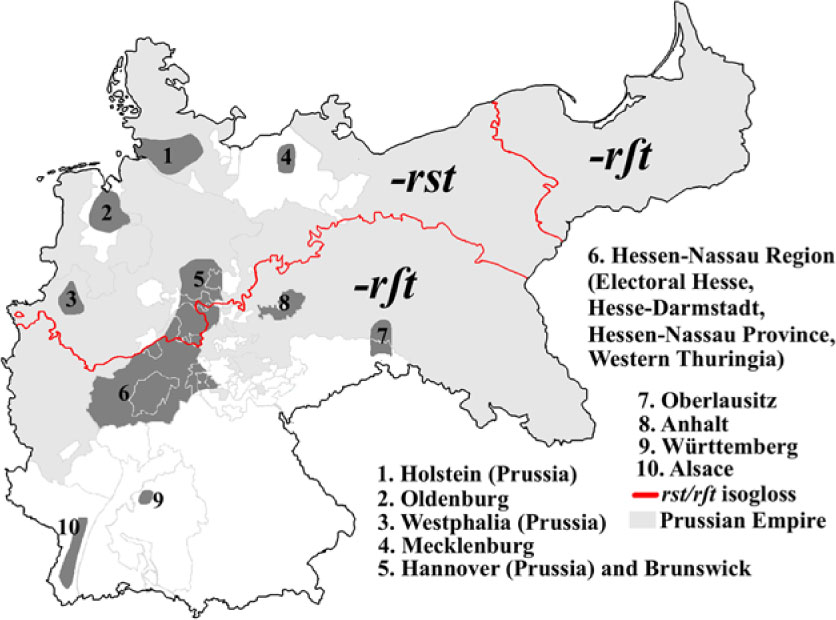
Map 2. Sibilant pronunciation in Wurst and the origin of German settlers
The dark grey areas represent the major sources of immigrants from Germany to Texas according to Jordan (Reference Jordan1966:33). Jordan uses 1860 and 1870 US Census data in central Texas counties for his analysis. For the eastern Texas settlements, the bulk of immigration was from northwestern and north-central Germany. For the western Texas settlements on the frontier (Jordan, Reference Jordan1966:123), an immigration society with roots in the Hessen-Nassau region of central Germany sponsored initial immigration. Based on Jordan’s figures and the isogloss from the Wenker atlas (Jordan, Reference Jordan1966:64, 123), Table 2 shows the estimated percentage of immigrants from regions in which the s-variant for Wurst is dominant (Hannover, Brunswick, Mecklenburg, Oldeburg, Lippe-Detmold, Hamburg, Hannover, Bremen) and regions in which the ∫-variant is dominant (Saxony, Anhalt, Baden, Württemberg, Hesse, Nassau, Bavaria, Saxe-Meiningen, Saxe-Weimer).
Table 2. Pronunciation of Wurst in immigrant donor dialects

The main difficulty in determining the exact proportionality of features is that nearly half of the respondents listed “Prussia” as their place of origin, which could indicate any of the provinces of the Prussian Empire (the light grey area in Map 2). Jordan notes that this includes immigrants from Westphalia, Holstein, parts of Hannover, Hesse, and Nassau, and in particular the Wetzlar-Braunfels area of Hesse that supplied many of the immigrants to the western settlements. The ∫-variant was likely the dominant form in the donor dialects listed as “Unspecified Prussia,” and in the dialect mixture as a whole. Therefore, Table 2 gives us a lower bound: a minimum of 23% of the immigrant population came from areas with the s-variant for Wurst, with a somewhat higher percentage in the eastern settlements.
Trudgill’s model predicts that the ∫-variant for Wurst will eventually replace the s-variant. Previous research in New Braunfels indicates the presence of variation, but with some evidence of focusing: Gilbert (Reference Gilbert1972) found that 87% of the speakers used the ∫-variant, and Boas (Reference Boas2009) found a higher proportion of 94% for his respondents three decades later.
For the other words, Haarbürste and Donnerstag, Gilbert found the s-variant to be more prevalent in New Braunfels, and in fact it was in the majority for Donnerstag. In both cases Boas found an increase in the usage of the ∫-variant. These findings are summarized in Table 3, which is culled from Boas (Reference Boas2009:153). For Donnerstag, this goes against the expectation that the majority form will overtake the minority form.
Table 3. Proportion of ∫- to s-variants in New Braunfels

Boas writes that “the change could be explained in terms of leveling, where in the mid-20th century Donnerstag was one of the few words for which the majority of informants still preferred [s] over [∫] in this consonant cluster. By the beginning of the 21st century, the almost exclusive use of [∫] in this context was extended from other words to Donnerstag” (Boas, Reference Boas2009:154). Boas also notes that in open interviews some speakers use an ∫-variant for erst (‘first’), which did not originally vary.
In the current analysis, I examine the distribution of Wurst, Haarbürste, and Donnerstag variants from all forty-four different Texas counties for which we have data.
3. Study
The data for this analysis come from recorded questionnaires which were collected between 2004 and 2016 by the TGDP. A typical interview session consists of a brief survey on the background and language attitudes of the speaker, an open interview in German on any topic, and the elicitation of the Gilbert and/or Eikel questionnaires. For these questionnaires, the speaker is prompted with a word or sentence in English and asked to provide a translation in Texas German. Each survey consists of approximately 200 questions. Boas et al (Reference Boas, Pierce, Weilbacher, Roesch and Halder2010) is a comprehensive description of the workflow of the TGDP. I compiled the responses to those questions in the Gilbert questionnaire for s/∫-alternations in the words Haarbürste ‘hairbrush’, Donnerstag ‘Thursday’, and Wurst ‘sausage’. I examined the same questions listed in Boas (Reference Boas2009). For this questionnaire, questions (1) and (16) are identical, as are (15) and (113). The relevant words are in bold:
1: A hairbrush
14: Thursday
15: He took the most sausage.
16: A hairbrush
113: He took the most sausage.
These tokens came from untranscribed audio recordings from the TGDP database.Footnote 4 The determination of whether a particular token instantiated the s-variant or the ∫-variant was made by aural inspection. I used a self-written Python computer program which played every recorded response for a particular question without any identifying information and in a randomized order. I excluded responses which contained neither variant, but I included compounds and variant pronunciations of vowels. For example, for Haarbürste (‘hairbrush’), I made the determination based entirely on the quality of the sibilant and included variations like Birste, Haarberst, Kaambürst (‘comb-brush’), etc. I checked my judgments with a non-German speaker, who was presented with 10% of the tokens for each question. Our judgments were in agreement for 97.1% (100/103) of these tokens.
From the biographical questionnaire forms filled out by each informant I recorded gender, year of birth, and county of birth. The collected data come from 486 informants (193 female, 282 male, and 10 other/undetermined). There were 130 uniquely listed birthplaces in 45 different Texas counties. These speakers were born between 1908 and 1979 with a median birth year of 1933. Most informants were born in rural communities, and informants typically described place of birth with reference to either the name of a small town or settlement (e.g., “Converse,” “Warda”), or county (“Lee County,” “Bexar County”), or orientation with respect to a town or city (“13 miles north of Fredericksburg”). I converted this information into geographic coordinates using the online geocoding tool at http://LatLong.net, a search function that provides geographic coordinates for cities, towns, and counties. There were 1068 tokens in total, of which 95 were excluded because a confident determination of the variant could not be made (454 for Wurst, 255 for Donnerstag, and 264 for Haarbürste).
3.1 Nested model comparison
In order to determine which predictors may characterize rst-alternation, I considered the following variables for each token:
Dependent Variable:
Value (i.e., [s]/ [∫])
Predictors:
1. Word (Haarbürste, Donnerstag, Wurst)
2. Gender of Speaker (Male, Female, none)
3. Speaker’s Year of Birth
4. Speaker’s Place of Birth
5. Speaker ID Number
Any of these four predictors could plausibly correlate with the observed feature variation. However, if the feature variation is evenly distributed and stable in the population, then Place of Birth and Gender will not be significant predictors. Year of Birth (YOB) may be a significant predictor. This would indicate phonological change over the course of the generations represented in the survey. The dependent variant Value is coded as a binary variable (s = 0, ∫ = 1). Word, Gender, and Speaker ID are categorical variables. I set “Wurst” as the reference for the Word variable and “F” as the reference for the Gender variable. Year of Birth (YOB) is coded as a continuous variable, and Place of Birth is coded with two continuous variables Latitude and Longitude. I scaled and z-normalized the three continuous variables in order to compare the effect sizes of each variable. I used the 800 tokens that contained no missing data (some respondents did not record their age or birthplace).
I determined which predictors are significant by comparing logistic regression models pairwise to determine which model best fit the data. I used the Akaike Information Criterion to compare model fitness (AIC; Akaike, Reference Akaike1974). A lower AIC, taken to be a reduction of at least 2, means that the added complexity of the model is warranted given the goodness of fit. First, I ran a generalized logistic regression in R (R Core Team, 2017). I used the predictor variables Word, Gender, YOB, Latitude, and Longitude. I compared this with a mixed-effect logistic regression with the same predictors and with Speaker ID as a random effect variable. I ran this using the glmer package in R (Bates et al, Reference Bates2014).
The purpose of this comparison is to see whether the model improves significantly when individual speaker variation is taken into account. Table 4 is a comparison of the results of these two models. The mixed-effect model performs decidedly better (AIC = 412.9, compared to 462.9), which indicates that the speakers are not a homogenous group. The mixed-effect model is a better fit. The only significant predictor at this level of complexity comes from a Word variable.
Table 4. Model Comparison of Generalized Linear Model with Mixed Effect Model for all variables

In order to determine which variables are significant, I performed a nested model comparison of mixed-effects models. I excluded each variable in turn and compared the AIC to the original model. Excluding Gender gave the greatest positive change in AIC (8.7), and so I conclude that a model which excludes Gender is a better fit. I then excluded each variable in turn from this new model, but the AIC improvement in each case was less than two. Therefore, the best fit was a model which removed Gender from consideration, leaving Word, Latitude, Longitude and YOB. This indicates that Word, Latitude, and Gender are allpotentially significant variables. Table 5 is a summary of this model.
Table 5. Mixed Effects Model with Word, YOB, Longitude, and Latitude

Word is the only variable with a significant correlation. In order to evaluate the robustness of these correlations, I also conducted a bootstrapping resampling on the correlation coefficients, drawing randomly with replacement for 1000 iterations. The result of this analysis is in Table 6. If the coefficient of a variable ranges between positive and negative values, this indicates that the variable is not significant. From this I conclude that the only variable that significantly correlates with the pronunciation of sibilants in rst-clusters is the lexical item elicited (Word). I did not find a correlation with Gender, Year of Birth, or Birthplace.
Table 6. Coefficient Correlation Confidence Intervals (Bootstrap Resampling of 1000 iterations

3.2 Variation and word, gender, and year of birth
The nested model comparison tells us that the only significant predictor of the sibilant feature is the word in which the feature is used. In particular, the word Donnerstag (‘Thursday’) was significant. This is an expected result, if we consider that Boas (Reference Boas2009) found Wurst (the reference factor) and Haarbürste to have a similar proportionality in contrast to Donnerstag. Each of the words have their own distribution, and it is necessary to consider each word separately in the analysis to follow. Strikingly, the overall proportionality of each word across the entire dataset is practically identical to that described in Boas (Reference Boas2009) for the community of New Braunfels, as can be seen in Table 7.
Table 7. Overall Percentage of ∫-variant by Lexical Item

While it is true that New Braunfels as a single community is well-represented in the dataset (13.7% of the tokens come from speakers who were born in New Braunfels, and 20.0% of the tokens come from speakers who were born elsewhere in Comal County), the close correspondence suggests that New Braunfels is a good proxy for Texas German as a whole, at least with respect to this particular feature. It would be interesting to see whether this is the case for the other features described in Boas (Reference Boas2009).
The statistical analysis did not find gender to be a significant factor. In the study sample, 44% of the speakers were female and 52% were male. Table 8 shows the results.
Table 8. Overall Percentage of ∫-variant by Gender

We expect a general trend toward the leveling out of the s-variant over time. However, the statistical analysis did not find Year of Birth to be a significant predictor, which would be expected if this leveling out is the result of an ongoing phonological trend. Gilbert (Reference Gilbert1972) and Eikel (Reference Eikel1954) indicate that the relative proportionality of the ∫-variant was lower in previous generations than we find in the modern data. It may be the case that this phonological trend towards the leveling out of the ∫-variant which occurred in previous generations stabilized before the final generation. In other words, the variation in the current generation is stable variation which has continued from the oldest speakers to the youngest speakers in the current dataset. On the one hand, this fits with the idea from Boas (Reference Boas2009) that Texas German was following a path towards the complete leveling out of all variants, and during the third generation the massive social changes that led to the endangerment of Texas German caused it to “freeze” in its development. However, this is separate from the question of whether these variants have become sufficiently distributed geographically so as to constitute a new dialect, because stable variation may also occur in a relatively homogenous language.
3.3 Individual speaker variation in the open interviews
The relative intra- and interspeaker variation is important for a proper understanding of the mechanisms of dialect formation. In particular, it would be useful to know how much variation can be attributed to variation within a single speaker. If most of the variation in variant choice is attributable to the speaker, and the individual differences between speakers are relatively small, then this would be evidence for focusing. Texas German has focused into a unary dialect with a probabilistic distribution of feature variants.
Gilbert (Reference Gilbert1972) recorded that one of his fifteen informants produced Wurst variably with either [s] or [∫], and that one of his fifteen informants produced Donnerstag variably. It is unclear if this is the same individual in both cases, but in any case there is reason to believe that some Texas German speakers produce these lexical items variably.
The survey results are not ideal for studying feature variation, because the questionnaires have only a few examples of multiple tokens of the same type from the same informant (there were two questions each for Haarbürste and Wurst). The items with multiple representations are those for which the ∫-variant is nearly 20 times as common as the s-variant. Considering the low number of tokens per type, it is almost certain that the level of intraspeaker variation will be underestimated by the survey.
To get a better understanding of individual speaker variation, I analyzed the distribution of rst clusters from the open interviews separately. The open interviews are longer recordings of conversations between the interviewer and the respondent on any topic. The majority of respondents describe growing up on a farm in the Texas Hill Country, speaking German at home and learning English for the first time in school. A substantial proportion of these interviews have been transcribed and annotated. I used the concordancer tool at the online Texas German Dialect Archive to search through the transcribed open interviews (Speaker IDs 1 - 395). I collected every word which was transcribed with an “rst” cluster (1332 tokens) or an “rscht” cluster (300 tokens).
By far, the most common rst-word in the open interviews is erst (‘first’). Including all derived forms and the adverb zuerst, this word appears 758 times in the corpus. The word is common in narratives about growing up in the Texas German belt.
The most common noun with an rst cluster is Wurst (‘sausage’). Including types of sausage (Blutwurst, Fleischwurst, Knackwurst, etc.) and other compounds (Wurstfest, Wurstkäse, Wurststube), the word appears 291 times in the corpus. Fredericksburg in particular is known for its yearly German cultural festival, Wurstfest. Discussions of tourism and development in modern-day Fredericksburg often mention the impact of this holiday. A great many speakers also discussed the process of preparing and smoking sausage at home.
Among the words analyzed in the surveys, Donnerstag appears only 13 times and a variant of Haarbürste appears once. The remaining words in the open interviews are (1) always pronounced with [∫] according to German phonology (verstehen, erstaunlich, Bürgersteig); (2) second-person verb forms (warst, erinnerst); or (3) English loanwords or code-switching in English (airstrip, understand, first).
I listened to every interview clip that contained an annotation “Wurst” or “Wurscht” and made a determination of whether the sibilant was an [s] or [∫]. Out of the 51 speakers, 42 of them used the word Wurst more than once for a total of 208 tokens (2–20 tokens per speaker, with a median of 3 and mean of 4.9). The results are presented in Table 9.
Table 9. Individual speaker variation in the ∫ and s-variants of Wurst

The percentage of mixed speakers is probably still underestimated. If the average speaker uses the s-variant only 5% of the time, they are unlikely to use it once in five tokens. The data is consistent with a pattern in which every speaker is a mixed speaker and uses both variants. It is also consistent with a pattern in which there are exclusively ∫-variant speakers and a minority of mixed speakers.
Boas (Reference Boas2009) mentions that the ∫-variant pronunciation has apparently spread to the word erst for some speakers, although the s-variant is still in the majority. I also searched the transcribed open interviews for the annotations “erst” and “erscht.” While I was not able to audibly verify the annotations in most cases, the transcriptions were generally perceived to be correct. If a bias exists, it will be towards the Standard German spelling “erst.” Out of 100 speakers, 89 used the word erst more than once, for a total of 774 tokens (2–38 per speaker with a median of 7 and a mean of 8.7). The results are in Table 10.
Table 10. Individual speaker variation in the ∫ and s-variants of erst

This is consistent with a pattern in which the majority of speakers are exclusive s-variant users and about one-fifth are mixed speakers. This means that some focusing has occurred, but speakers are not a completely homogenous group—some speakers behave differently from others. I now turn to the question of whether these differences manifest geographically, meaning that different communities express different patterns, or if this variation is distributed homogenously throughout the Texas German belt.
3.5 Variation and geography
Birthplace was not a significant predictor in the statistical model, but this will not tell us whether there are markedly different patterns in different communities. Table 11 shows the distribution for these variants in four representative counties: Gillespie and Comal in the west and Fayette and Lee in the east.
Table 11. Percentage of ∫-variant by word in four major counties

Overall the percentages are similar in each county, but there are some basic differences: Donnerstag appears to be nearly leveled out in the east, and the s-variant for Wurst is unusually common in Comal County. But we cannot tell from the data if these are statistically reliable patterns. In order to see whether there are reliable patterns, we need to look at measures of spatial autocorrelation.
3.6 A Demonstration of spatial autocorrelation
To examine the question of whether sibilant variation is diffused geographically, I first consider an unrelated feature of Texas German that does exhibit a clear clustering pattern of regional variation. In contrast to sibilant variation, there are certain lexical items which are clearly associated with certain regions. The feature presented here is the lexical item for “pumpkin,” Kurbis in Standard German. I analyze this feature as a general demonstration of spatial autocorrelation statistics before moving on to sibilant variation. The data come from another question elicited by the Gilbert survey:
125. A pumpkin (the fruit of Cucurbita pepo)
Table 12 depicts the most common variants for this lexical item. The most common term is Bungis (including variants Pungis, Bunkis). The next most common term is an English loanword Pumpkin. The term Galawas (Galavasa, Galawa) is associated particularly with the Alsatian Texas German of Castroville and Medina County. Because many speakers report the same birthplace, some points in Map 3 represent multiple tokens.
Table 12. Variation in the lexical item “Pumpkin”


Map 3. Distribution of variants for “Pumpkin”
Bungis appears to be the most common variant in the western settlements (excluding the influence of Alsatian Texas German in the southwest), while Pumpkin dominates in the eastern settlements. We can test the statistical reliability of these clusters with measures of global and local spatial autocorrelation using the Moran’s I and Getis-Ord G* statistics (Grieve et al, Reference Grieve, Speelman and Geeraerts2011; Zanuttini et al, Reference Zanuttini, Wood, Zentz and Horn2018; Tamminga, Reference Tamminga2013).
The Global Moran’s I statistic is useful for determining whether there is an overall pattern of regional clustering of a feature variant. Using ArcMap’s Moran’s I tool, I tested the comparative regional distribution of the two major variants Bungis and Pumpkin (coding them as 1 and 0 respectively). I used a fixed band with a specified cut-off distance (Grieve et al, Reference Grieve, Speelman and Geeraerts2011). This cutoff distance corresponds to the resolution of the clusters: a low cutoff is better for identifying small clusters, and a higher cutoff is better for identifying large clusters. Table 13 shows the Moran’s I analysis for Bungis/Pumpkin at ten different cutoff distances from 20 kilometers to 200 kilometers (60 kilometers is roughly the size of a county, and 200 kilometers is about half the overall length of the German belt).
Table 13. Moran’s I Analysis for Bungis/Pumpkin

The Moran’s I statistic ranges from −1 to 1. A score close to 0 indicates that the feature is scattered randomly throughout the region. 1 indicates the maximum level of regional clustering, and −1 indicates that the variable is maximally dispersed. For every tested cutoff distance, there is a highly significant result indicative of a pattern of regional clustering.
For local autocorrelation, I used the Getis-Ord Gi* statistic with ArcMap’s hotspot analysis tool (Ord & Getis, Reference Ord and Getis1995, Reference Ord and Getis2001). For each data point, this statistic determines the degree to which it is surrounded by similar values. Regional clusters show up as “hot spots” or “cold spots.” I ran the statistic on several fixed-band cutoff distances and found 60 kilometers to be representative of the general pattern. In Map 4, I created a boundary around points with a confidence interval of 95% or greater (I used the Thiessen polygon tool to partition the map into regions defined by distance to the closest data point). These can be thought of as isogloss boundaries for Bungis (hot spot) and Pumpkin (cold spot).

Map 4. Hotspot analysis for Bungis/Pumpkin

Map 5. Hotspot analysis for Haarbürste

Map 6. Hotspot analysis for Wurst
3.7 Spatial clustering of rst-variation
Returning to the rst variants, I performed the same analysis for each of the three words Wurst, Donnerstag, and Haarbürste. The global autocorrelation analysis for each word is presented in Table 14.
Table 14. Moran’s I Analysis for Wurst, Donnerstag, and Haarbürste

One of the three words, Donnerstag, shows a pattern consistent with a random distribution at every cutoff distance. We can conclude that the distribution of sibilant variants in Donnerstag is homogenous in the Texas German belt.
The other two words show a pattern consistent with randomness (or even dispersal) at higher resolutions, but they both show significant results for clustering below 60 kilometers. This means that there is no widescale pattern, but we may find significant clustering at the level of particular counties or settlements. I ran a hotspot analysis on Wurst and Haarbürste with a fixed band cutoff corresponding to the highest Moran’s I p-value (20 kilometers for Wurst and 40 kilometers for Haarbürste) to maximize the potential to pick out hot spots.
The only clustered areas are in the west. The cold spot in the south is somewhat outside the German belt and corresponds to single judgments, so it may be considered noise. The cold spot in the north is centered near the settlement of Fredericksburg, and the hot spot is centered near the settlement of New Braunfels. These correspond to relatively low and high percentages of the ∫-variant in Haarbürste in these communities. We find the reverse situation for Wurst.
Again, there are cold spots corresponding to single judgements from speakers born outside the traditional area of the German belt. These can be excluded from analysis. We find a cold spot centered around New Braunfels and a hot spot centered around Fredericksburg, corresponding to relatively low and high percentages of the ∫-variant for Wurst in these communities.
The two words for which we do have some evidence for spatial clustering are both words in which the overall average percentage for the ∫-variant is about 95%. In Fredericksburg, the relative cold spot for Haarbürste corresponds to a proportion of 91%, while in New Braunfels, the relative cold spot for Wurst corresponds with a proportion of 83%. This low result is somewhat surprising considering that Boas (Reference Boas2009) found a proportion of 94%. In any case, these communities do not appear to have substantially different patterns of rst variation.
Considering the geographic distribution of German donor dialects to central Texas, we would expect broad differences between east and west, as was clearly evident in the variant lexical items for “pumpkin.” The eastern settlements should have a higher percentage of the s-variant because more settlers came from northern Germany to these areas, while the ∫-variant should predominate in the western settlements. We might also expect the southeast to have a different pattern due to the influence of Alsatian German. We do not find this, but rather a much more homogenous pattern, particularly in the east, with marginal differences between New Braunfels and Fredericksburg in the west.
I conclude that for rst variation, the distribution of variation is reasonably uncorrelated with geographic region. This variation looks more like stable variation in a homogenous Texas German variety than variation between subvarieties.
Conclusion
The presence of variation in a particular linguistic variety may be correlated with many different factors. For the variable pronunciation of rst-clusters in Texas German, I have examined the possibility that it may be correlated with particular lexical items or with some speaker feature such as age, gender, or place of birth. Texas German is an endangered dialect, and some variation should be expected due to the chaotic processes of language attrition. For this particular feature, however, and for other phonological features examined by Boas (Reference Boas2009), the diachronic tendency has been in the direction of uniformity. Boas emphasizes the striking lack of increased variability that might be expected in a situation of language death (Sasse, Reference Sasse1992): most of the trends of phonological variation described by Gilbert (Reference Gilbert1972) are found in Boas (Reference Boas2009), and in fact leveling processes have continued in the same direction, but are not yet completed. The ∫-variant has virtually replaced the s-variant for some lexical items, continuing a trend noted in Gilbert (Reference Gilbert1972).
It is clear that different lexical items are associated with different levels of variation among the three lexical items Haarbürste, Donnerstag, and Wurst. This pattern has been extended to other words with this cluster, as in erst. An examination of intraspeaker variation in the open interviews indicates that the speakers are not a homogenous group: in regular speech some speakers appear to use the majority form exclusively, while other speakers use the markers variably. This heterogeneity is reminiscent of East Sutherland Gaelic, in which there is stable local variation.
I found no statistical correlation between gender or age and the expression of particular variants. Taken together, these findings suggest a lack of diachronic change for these variants in the recent history of Texas German. If this is broadly the case, then the variation present in modern-day Texas German is relatively stable. This can be taken either as an argument that the dialect formation process has completed and converged on a variable pronunciation, or else that the process was interrupted before a final invariant pattern could emerge.
I have argued that the question of whether a group of dialects have cohered into a new dialect cannot be answered by the mere presence of variation, but should rather be answered by the geographic distribution of variant proportions. This is because variation of many types can exist in a homogenous language community. The factors that allow for a minority variant to survive as a stable variant in the new dialect remain to be explored, but the important issue is that the end state should be measured by the sufficient diffusion of variant proportions across the dialect region.
The geographic analysis of variation in rst-clusters show a pattern characteristic of a randomly scattered feature, with no regions with statistically higher or lower proportionality. An expected pattern for non-convergence would be multiple hotspots corresponding to particular settlement patterns, and by and large this is not what I found with this feature. However, the current study has explored a single variant in depth, and it would be necessary to look at other variant features in order to determine whether Texas German appears to be more or less homogenous. Certain lexical items such as the word for “pumpkin” are clearly associated with particular regions of the German belt. It would also be helpful to compare this analysis with other linguistic enclaves to see what a thoroughly heterogenous dialect community would look like. The analysis of this particular feature demonstrates how these techniques may be applied to other variant features in Texas German in order to provide an overall picture of the uniformity or heterogeneity of the dialect region.


