


Introduction
Among the poorest 80% of contemporary humanity, increasing income on average leads to increasing body weight (Hruschka et al., Reference Hruschka, Hadley and Brewis2014) – a finding that has been confirmed across the world’s major regions (Hruschka, Reference Hruschka, Anderson-Fye and Brewis2017). The positive correlation between economic resources and body size fits a simple model: more economic resources permit individuals to consume more calories and engage in less physical labour, thereby depositing more fat (Brown & Konner, Reference Brown and Konner1987; Eaton et al., Reference Eaton, Konner and Shostak1988; Hruschka Reference Hruschka2012). However, in many high-income countries, the relationship between body mass index (BMI) and economic resources often reverses (Dinsa et al., Reference Dinsa, Goryakin, Fumagalli and Suhrcke2012; Hruschka, Reference Hruschka, Anderson-Fye and Brewis2017). Specifically, in these contexts, heavier individuals on average live in lower-income households – a phenomenon often referred to as the ‘reverse gradient in obesity’ (Sobal & Stunkard, Reference Sobal and Stunkard1989; Monteiro et al., Reference Monteiro, Conde, Lu and Popkin2004; Subramanian et al., Reference Subramanian, Perkins, Ozaltin and Smith2011; Dinsa et al., Reference Dinsa, Goryakin, Fumagalli and Suhrcke2012; Hruschka, Reference Hruschka2012). This body mass reversal has been observed across all major world regions, except perhaps South Asia and Polynesia (Hruschka, Reference Hruschka, Anderson-Fye and Brewis2017; Choy et al., Reference Choy, Hawley, Naseri and McGarvey2020).
The puzzling reversal of the relationship between income and BMI in high-income countries has inspired a number of theoretical explanations (Sobal & Stunkard, Reference Sobal and Stunkard1989; Dinsa et al., Reference Dinsa, Goryakin, Fumagalli and Suhrcke2012; Hruschka, Reference Hruschka, Anderson-Fye and Brewis2017). This is in part because the origins of the reverse gradient are highly relevant to theories of how social stratification and human biology interact to create observed disparities in health and achievement (Sobal & Stunkard, Reference Sobal and Stunkard1989; House, Reference House2002; Olafsdottir, Reference Olafsdottir2007; Phelan et al., Reference Phelan, Link and Tehranifar2010). They are also of particular interest to policymakers and public health practitioners aiming to reduce health disparities and to alleviate the disease burden of obesity (Drewnowski, Reference Drewnowski2009).
Most current explanations posit that greater income gives people the ability to achieve society’s ideals for body size and shape, while individuals living in lower-income households do not have the economic capacity to do so. For example, Sobal and Stunkard (Reference Sobal and Stunkard1989, p. 266) suggested a large body size might be a ‘sign of health and wealth’ in poorer countries, but in wealthier settings, this can shift from an ideal to a stigmatized condition. As these ideals shift, wealthier individuals also use their economic capacity to attain the new thin ideal. Sobal and Stunkard did not commit to the specific mechanisms by which people with higher incomes were better able to approximate body size ideals. Recently, however, scholars have provided a number of more fully elaborated accounts based variously on food choice constraints, leisure exercise opportunities and time pressures on food preparation (Hruschka, Reference Hruschka2012). Two recurring assumptions of these deprivation theories are that (1) people actively work to change their bodies to fit current ideals, and (2) people with greater income can change their body size by consuming the costly foods and engaging in the physical activity necessary to achieve those ideals.
Although deprivation theories have been the favoured source of explanations for the reverse gradient in obesity, a second class of theories based on anti-fat discrimination are also potentially relevant. Such theories reverse the direction of causation and posit that anti-fat discrimination in hiring and marriage can lead individuals with higher BMI to be selected into lower-paying jobs and lower-income households (Cawley, Reference Cawley2004; Conley & Glauber, Reference Conley and Glauber2007; Glass et al., Reference Glass, Haas and Reither2010; Mason, Reference Mason2012; Malcolm & Kaya, Reference Malcolm and Kaya2016; Oreffice & Quintana-Domeque, Reference Oreffice and Quintana-Domeque2016). Such discrimination can happen for a range of reasons, including preferences for attractive partners and employees and weight-based judgments of competence and motivation that can affect both educational opportunities and hiring (Crandall & Schiffhauer, Reference Crandall and Schiffhauer1998; Greenberg et al., Reference Greenberg, Eastin, Hofschire, Lachlan and Brownell2003; Puhl & Brownell, Reference Puhl and Brownell2003; Crosnoe & Muller, Reference Crosnoe and Muller2004; Puhl et al., Reference Puhl, Andreyeva and Brownell2008; Puhl & Heuer, Reference Puhl and Heuer2009; Glass et al., Reference Glass, Haas and Reither2010; Flint & Snook, Reference Flint and Snook2014). Notably, explanations based on anti-fat discrimination do not require that individuals have any capacity to manipulate their own weight. Rather, discrimination theories simply assume that there is some pre-existing BMI variation in the population and that anti-fat discrimination selects thinner individuals into higher-income jobs or higher-resource households. In turn, this selection process creates a negative correlation between BMI and household economic resources.
Despite their potential relevance, such anti-fat discrimination theories have rarely been proposed as explanations in the hundreds of papers currently published on the reverse gradient in obesity. And although a number of studies demonstrate such anti-fat discrimination in both marriage and labour markets, it is not clear whether such discrimination could create reverse gradients of the magnitude observed in high-income countries (Baum & Ford, Reference Baum and Ford2004; Cawley, Reference Cawley2004; Oreffice & Quintana-Domeque, Reference Oreffice and Quintana-Domeque2010; Judge & Cable, Reference Judge and Cable2011; Ponzo & Scoppa, Reference Ponzo and Scoppa2015). One key challenge in comparing the explanations from deprivation and discrimination theories is that they often make identical empirical predictions, and isolated tests of these predictions against simple null hypotheses cannot differentiate between these explanations. This paper seeks: (1) to unite these two theoretical literatures to identify one set of contrasting predictions related to the reverse gradient in obesity and (2) to assess the relative agreement of these contrasting predictions with data from representative samples of men and women in two high-income countries with high levels of anti-fat discrimination: the United States and South Korea (Crandall & Schiffhauer, Reference Crandall and Schiffhauer1998; Schewekendiek et al., Reference Schwekendiek, Minhee, Ulijaszek and Schwekendiek2013). Data were analysed from these two countries to assess the consistency of results across two culturally distinct countries where a reverse gradient has been observed.
Deprivation and obesity
Current explanations for the reverse gradient in obesity nearly exclusively derive from some version of a deprivation-based theory (Parsons et al., Reference Parsons, Power, Logan and Summerbelt1999; Giskes et al., Reference Giskes, Lenthe, Turrell, Kamphuis, Brug and Mackenbach2008; Drewnowski, Reference Drewnowski2009). These represent a broader class of theories for health disparities which posit that increasing resources should give individuals more opportunities to achieve healthier outcomes (Adler & Newman, Reference Adler and Newman2002; Pampel et al., Reference Pampel, Krueger and Denney2010). Researchers have proposed a number of mechanisms that could increase the risk of obesity among poorer individuals. For example, the ‘energy density hypothesis’ is built on the observation that foods lower in energy density (such as vegetables) can protect against obesity but also cost more per calorie. Consequently, wealthy individuals are best able to consume the costly diets necessary to fit an ideal of thinness (Drewnowski & Specter, Reference Drewnowski and Specter2004; Drewnowski & Darmon, Reference Drewnowski and Darmon2005; Drewnowski, Reference Drewnowski2009). A related theory, the ‘protein leverage hypothesis’, is built on the observation that protein costs 20 to 50 times more per calorie than other macronutrients, such as fat and carbohydrates. Evidence also suggests that protein is more satiating than other macronutrients and humans will continue to consume food until they have reached a certain amount of protein. Accordingly, in low-income situations, individuals will purchase cheaper low-protein alternatives that do not satiate and thus encourage consumption of excess calories (Simpson & Raubenheimer, Reference Simpson and Raubenheicmer2005; Brookes et al., Reference Brooks, Simpson and Raubenheimer2010). A third argument focuses on economic constraints on physical activity by proposing that wealthier individuals have more of the kinds of opportunities for physical activity – including leisure time as well as safe public and private spaces for exercise – needed to shape their bodies to fit society’s ideals (Gordon-Larsen et al., Reference Gordon-Larsen, Nelson, Page and Popkin2006). A unifying assumption of all of these theories is that people can effectively deploy additional economic resources to lose weight or maintain a lower weight, and that people who do not have these resources are constrained in their ability to do so.
These different deprivation hypotheses have empirical support in a large and growing number of cross-sectional studies (Drewnowski, Reference Drewnowski2009). However, finer-grained tests of these theories examining historical trends or using mediation analyses have shown mixed results. For example, one analysis of BMI trends over three decades in the US suggests that increased portion size and more frequent eating were more important factors than the energy density of food in increasing BMI in the US (Duffey & Popkin, Reference Duffey and Popkin2011). Moreover, the energy density of foods does not appear to account for a very large proportion of the effect of social class on obesity (Aggarwal et al., Reference Aggarwal, Monsivais, Cook and Drewnowski2011). When focusing on protein, instead, experimental and population-based studies have shown either (1) no effect of protein on energy intake and obesity, or that (2) these effects depend on specific kinds of protein (Blatt et al., Reference Blatt, Roe and Rolls2011; Bujnowski et al., Reference Bujnowski, Xun, Daviglus, Van Horn, He and Stamler2011; Lin et al., Reference Lin, Bolca, Vandevijvere, De Vreise, Mouratidou, De Neve and Polet2011; Vinknes et al., Reference Vinknes, de Vogel, Elshorbagy, Nurk, Drevon and Gjesdal2011). In historical perspective, very few cases of longitudinal increases in economic resources are associated with longitudinal declines in BMI over the same period of time (Hruschka, Reference Hruschka2012). Thus, although cross-sectional associations of income with obesity are consistent with deprivation theories, finer-grained analyses based on longitudinal data and mediation analyses show inconsistent results.
Anti-fat discrimination
Deprivation theories have been the dominant explanation for reverse gradients in obesity. However, a second class of theories based on anti-fat discrimination might also account for the observed negative associations between BMI and income (Averett & Korenman, Reference Averett and Korenman1996; Averett et al., Reference Averett, Sikora and Argys2008; Chiappori et al., Reference Chiappori, Oreffice and Quintana-Domeque2012; Conley & Glauber, Reference Conley and Glauber2007; Morris, Reference Morris2007; Mukhopadhyay, Reference Mukhopadhyay2008; Oreffice & Quintana-Domeque, Reference Oreffice and Quintana-Domeque2010; Glass et al., Reference Glass, Haas and Reither2010). In the last three decades, social scientists and public health researchers have consistently documented anti-fat discrimination in the US and in European countries (Crandall & Schiffhauer, Reference Crandall and Schiffhauer1998; Greenberg et al., Reference Greenberg, Eastin, Hofschire, Lachlan and Brownell2003; Chen & Brown, Reference Chen and Brown2005; Puhl et al., Reference Puhl, Andreyeva and Brownell2008; Puhl & Heuer, Reference Puhl and Heuer2009; Flint & Snook, Reference Flint and Snook2014). Not thoroughly studied quantitatively yet, South Korea also serves as a useful case study of weight discrimination with its extremely high level of weight stigma against big body sizes (Jung & Lee, Reference Jung and Lee2006; Marini et al., Reference Marini, Sriram, Schnabel, Maliszewski, Devos and Ekehammar2013; Schwekendiek et al., Reference Schwekendiek, Minhee, Ulijaszek and Schwekendiek2013).
Two possible pathways could explain how anti-fat discrimination could give rise to the observed reverse gradient in obesity. Labour market discrimination in the processes of hiring, promotion and retention is one potential pathway leading individuals with higher BMIs to have lower personal incomes. Body mass index is a specific example of a wider range of individual physical characteristics, including height and facial attractiveness, that appear to garner premiums or incur penalties in labour markets (Averett & Korenman, Reference Averett and Korenman1996; Glass et al., Reference Glass, Haas and Reither2010). Numerous studies in the US and Europe have demonstrated how BMI can influence salaries, especially among women (Baum & Ford, Reference Baum and Ford2004; Cawley, Reference Cawley2004; Judge & Cable, Reference Judge and Cable2011). However, it is not clear whether such discrimination can generate gradients of the magnitude observed in the US and other countries (Hruschka, Reference Hruschka, Anderson-Fye and Brewis2017).
Anti-fat discrimination in the marriage market is another pathway that can generate negative correlations between BMI and household income. As opposed to labour market discrimination, marital discrimination should theoretically lead to negative correlations between BMI and a spouse’s income (or overall household income), but not necessarily personal income. This has been shown empirically in a number of studies (Taylor & Glenn, Reference Taylor and Glenn1976; Udry, Reference Udry1977; Stevens et al., Reference Stevens, Owens and Schaefer1990; Burdett & Coles, Reference Burdett and Coles2001; Carmalt et al., Reference Carmalt, Cawley, Joyner and Sobal2008; Sassler & Joyner, Reference Sassler and Joyner2011; McClintock, Reference McClintock2014). The effects of both marital and labour market discrimination should be particularly pronounced in the highest income segments of contemporary humanity – those living in high-income countries, and high-wealth populations in middle- and even low-income countries – where increasing resources no longer bring appreciable increases in caloric consumption or related gains to body weight (Hruschka, Reference Hruschka2012; Hruschka et al., Reference Hruschka, Hadley and Brewis2014).
Substantial work in sociology has examined the various ways that partners in heterosexual marriages sort by income and physical characteristics and a range of other traits (McClintock, Reference McClintock2014; Ponzo & Scoppa, Reference Ponzo and Scoppa2015). The partner selection literature frequently distinguishes between matching on the same characteristics, such as partner similarity in education, income or height, and correlations across different traits, such as individuals with higher education marrying partners with higher incomes. Although same-trait matching and cross-trait correlations are sometimes depicted as the result of mutually exclusive processes – selecting partners based on similarity versus selecting partners based on desired traits – couples very likely engage in both (McClintock, Reference McClintock2014). In many situations, researchers have also found gender asymmetries in cross-trait matching. For example, a few recent studies have observed correlations between individual BMI and a partner’s income that are stronger for women than for men in heterosexual marriages (Oreffice & Quintana-Domeque, Reference Oreffice and Quintana-Domeque2010). However, this particular asymmetry does not necessarily mean that women do not prefer male partners with a lower BMI or that men do not prefer female partners with a higher income. Indeed, in this case, existing analyses suggest that both genders care about their partner’s BMI and salary, but to differing degrees (Oreffice & Quintana-Domeque, Reference Oreffice and Quintana-Domeque2010; Ponzo & Scoppa, Reference Ponzo and Scoppa2015). Rather, such asymmetries simply indicate that there are some quantitative rather than categorical gender differences in preferences and socially constrained endowments and opportunities. The roots of such differences in preferences are of considerable interest, and there are ongoing productive debates about their social structural and biological origins (McClintock, Reference McClintock2014).
Predictions
There are many ways that marriage, household income and weight can come to be related to each other, and mechanisms described in both of these theories may simultaneously play roles in creating such reverse BMI gradients (Pudrovska et al., Reference Pudrovska, Reither, Logan and Sherman-Wilkins2014). In many cases, these differing explanations for the reverse gradient – deprivation, labour market discrimination and marital discrimination – are all consistent with coarse-grained associations between income and BMI. Thus, it can be useful to identify contrasting predictions of the different theories as a way to compare them.
This study focuses on contrasting predictions about the association of household income with BMI among never-married women. Deprivation theories propose individuals with lower household incomes will have fewer opportunities to maintain a healthy weight through diet and exercise. Importantly, current descriptions of such theories do not explicitly make differing predictions based on whether someone has never married or is currently married. In either case, household income is considered a key driver of the association. Theories based on anti-fat discrimination in labour markets also do not explicitly make differing predictions about the relationship of household income and BMI for never-married or currently-married individuals. If higher individual BMI is leading to lower personal income, then higher individual BMI should also lead to lower household income. Crucially, explanations based on anti-fat discrimination in marriage do lead to contrasting predictions for never-married and currently-married individuals. Specifically, if anti-fat discrimination in heterosexual marriage can account for observed reverse gradients, then no correlation between household income and BMI should be observed among individuals who have never entered into a marriage (see Figure 1). Conversely, a negative correlation should be seen between household income and BMI among individuals who have entered into a marriage.

Figure 1. Predictions of three different explanations for the reverse gradient in BMI.
The expected direction of the association of household income and BMI under each theory is graphically summarized in Figure 1. Of crucial importance for this theoretical comparison is differences in the slopes relating household income and BMI, rather than simple mean differences in BMI between married and never-married individuals, might be due to marriage increasing BMI or BMI shaping the probability of getting married (Umberson et al., Reference Umberson, Liu and Powers2009; Glass et al., Reference Glass, Haas and Reither2010; Pudrovska et al., Reference Pudrovska, Reither, Logan and Sherman-Wilkins2014).
To compare these two explanations for the reverse gradient in obesity, their contrasting predictions were assessed in nationally representative samples from two high-income countries with very different cultural backgrounds – South Korea (2007–2014) and the US (1999–2006) – to see if the results generalized across diverse cultural contexts. The comparison focused on currently- and never-married individuals, because the discriminating predictions of the two theories are most clearly different for these two groups (see below). To replicate past analyses, a naïve analysis was first conducted without stratifying on marital status. Then the interaction between marital status and household income was examined to see if the reverse gradient was observed among both currently- and never-married individuals (consistent with deprivation theories) or was observed only among currently-married individuals (consistent with discrimination theories). Also a number of additional sensitivity analyses were conducted that assessed alternative hypotheses based on differences between currently- and never-married individuals in age, employment and motivation to manage their weight.
Methods
Samples
Two datasets were used for the analysis: the 1999 and 2014 National Health and Nutrition Examination Surveys (NHANES) and the Korean version of NHANES (2007–2014 KNHANES). The NHANES and KNHANES surveys were designed to examine the health and nutritional status of children, adolescents and adults living in the United States and South Korea, respectively (CDC, 2014; KCDC, 2014). To analyse patterns in Korea, KNHANES IV conducted in 2007–2009 (KCDC, 2007), KNHANES V conducted in 2010–2012 (KCDC, 2010) and KNHANES VI conducted in 2013–2015 (KCDC, 2013) were used. The 2015 data had not been released at the time of analysis, so the datasets between 2007 and 2014 were merged for the analysis. To analyse patterns in the United States, the continuous NHANES data collected between 1999 and 2014 were used.
The final sample included those Korean and American non-pregnant respondents in KNHANES and NHANES with ages between 20 and 49 years. Furthermore, only Non-Hispanic White participants were considered in NHANES as they have consistently shown a reverse gradient in obesity, and they comprised a large enough sample size for comparison with KNHANES (Hruschka, Reference Hruschka, Anderson-Fye and Brewis2017). Because South Korea is racially and ethnically homogenous with relatively few immigrants, ethnicity was not restricted for the analysis of KNHANES.
Limiting the samples to currently-married and never-married individuals provides the cleanest comparison of the predictions. Specifically, those who are never married have not had the opportunity to gain income through marriage whereas those who are currently married have a household income that most directly reflects income gains through marriage (as well as their own income). By contrast, individuals who are widowed or divorced may have household income that reflects gains from past marriages to an unknown degree (e.g. alimony or dividends from a spouse’s savings or pension). For this reason, those respondents who were divorced, widowed or separated at the time of the survey were excluded from the sample (4% of KNHANES and 12% of NHANES samples). Cohabitation was recorded in the NHANES, but not KNHANES, datasets, so analyses focused on formally-married versus never-married individuals (cohabiting individuals were 10% of US sample). As a result, the non-weighted final sample sizes were 20,823 (females=11,835 and males=8988) for KNHANES and 6395 (females=3089 and males=3306) for NHANES. Sensitivity analyses that stratified analyses by currently-married and never married were also conducted (Tables 7 and 8) and included cohabiting with currently-married individuals in the US sample (Table 9). The key findings did not change under these conditions.
Measures
Assessing BMI and obesity
Body mass index (BMI) was used as an outcome variable in the analysis. The reverse gradient is generally described using BMI, assuming that BMI is a good proxy for body fat (Sobal & Stunkard, Reference Sobal and Stunkard1989; Monteiro et al., Reference Monteiro, Conde, Lu and Popkin2004; Subramanian et al., Reference Subramanian, Perkins, Ozaltin and Smith2011; Dinsa et al., Reference Dinsa, Goryakin, Fumagalli and Suhrcke2012; Hruschka, Reference Hruschka2012; Hruschka & Brewis, Reference Hruschka and Brewis2013). However, body mass confounds fat mass with the rest of the body’s tissue, including bone, muscle and water. Thus, some caveats apply when interpreting BMI as a measure of fat. First, sex differences in body composition mean that women generally have larger quantities of (and variability in) body fat than men do. Conversely, men have larger quantities of, and variability in, lean mass. These differences in body composition mean that body mass is a closer proxy of body fat in women than in men (male R 2=0.78–0.85; female R 2=0.83–0.91) and that body mass in men more deeply confounds fat mass and fat-free mass (Hruschka et al., Reference Hruschka, Rush and Brewis2013). These sex differences are quite remarkable and have led to ample critiques of BMI as a proxy for body fat. However, once BMI is adjusted for these sex and population differences, it is a relatively good proxy for total body fat, especially for women (R 2=0.83–0.91) (Hruschka et al., Reference Hruschka, Rush and Brewis2013).
Income
In KNHANES, income level was measured by a total monthly average household income (unit=10,000 won). In NHANES, income level was measured by a Poverty Income Ratio (PIR) defined by the US Census Bureau. This income index measures the ratio of a household’s income to a set income threshold. For example, if a given family has a higher-than-average income, PIR will be greater than 1. If the family has a lower-than-average income, PIR will be less than 1. To interpret income effects as the increase in BMI per percentage increase in income, log income was analysed.
Covariates
Given that education can have effects on BMI independent of income, education was included as a covariate in analyses (Monteiro et al., Reference Monteiro, Conde and Popkin2001). In both NHANES and KNHANES, education level was grouped into three categories for a direct comparison across the two countries: less than high school education, high school graduate and college graduate or above. This grouping accounted for differences in the education system through high school between Korea and the US (6-3-3 system in Korea and 5-3-4 system in the US).
A number of covariates aimed at ruling out alternative hypotheses for observed patterns were also included. First, if an effect of income on BMI was observed among currently-married individuals, but not never-married individuals, this could have been due to greater motivation to lose weight among currently-married individuals. To assess the potential confounding role of motivation to lose weight, reported efforts to lose weight were controlled for. Second, an alternative account for this pattern is due to differences in employment status that can influence available time for weight maintenance. For example, if never-married individuals are more likely to have a job than currently-married individuals, they may be less likely to have the time necessary to translate higher income into better weight maintenance. To assess this possibility, current employment, as well as an interaction of current employment with household income, were included in the models. Third, married households in general will on average have higher incomes than non-married households due to the potential to have dual earners, so household size was controlled for as well. Fourth, pregnancy and childbirth can have long-term effects on BMI, and so available variables on parity (NHANES) and gravity (KNHANES) were included as a covariates for analyses of the women’s samples. Finally, as outlined in the sample section, the analyses controlled for race and ethnicity through sample selection.
Analysis methods
The ordinary least square (OLS) regression model was used for the analysis. Because multiple years were merged for both NHANES and KNHANES, an appropriate sampling weight provided by CDC and KCDC, respectively, was used to adjust each dataset for a different level of contribution from each year. For analysis, in SAS 9.4, PROC SURVEYMEANS and PROC SURVEYREG procedures with relevant options were used to consider a stratified multistage probability sampling design. In each procedure, the Not Missing Completely at Random (NOMCAR) option was used to include cases with missing values in analysis variables for variance estimation as recommend by both CDC and KCDC. In addition, the DOMAIN option was used in all procedures, instead of list-wise deletion, to calculate correct standard errors of estimates from the whole sample, not from subsamples. The results from sensitivity analysis with and without a sampling weight and the options in SAS procedures showed substantially identical results (see Tables 2 and 3 for weighted results and Tables 5 and 6 for non-weighted results).
Table 1. Summary statistics of main variables by gender, Korea (2007–2014) and USA (1999–2014)

a Won in Korea or Poverty Income Ratio (PIR) in the US samples.
b Gravidity in Korea.
c Full number of cases (pre-weight) including those with missing values in one or more variables since PROC SURVEYMEANS statement was used with NOMCAR and DOMAIN options; adjusted for sample weight; dummy variables for survey years omitted from table.
Table 2. Regression estimates of BMI on household income and marital and employment status, females, Korea (2007–2014) and USA (1999–2014)

a Gravidity in Korea.
b Full number of cases (pre-weight) including those with missing values in one or more variables since PROC SURVEYMEANS statement was used with NOMCAR and DOMAIN options.
*p<0.05; **p<0.01; ***p<0.001, two tailed; adjusted for sample weight; year effects are controlled but omitted.
Table 3. Regression estimates of BMI on household income, marital and employment status, males, Korea (2007–2014) and USA (1999–2014)

a The full number of cases (pre-weight) including those with missing values in one or more variables since PROC SURVEYMEANS statement is used with NOMCAR and DOMAIN options.
*p<0.05; **p<0.01; ***p<0.001; two tailed; adjusted for sample weight; year effects are controlled but omitted.
Table 4. Estimated effects of income on BMI by marital status, Korea (2007–2014) and USA (1999–2014)

95% Bonferroni adjusted confidence intervals in parentheses; adjusted for sample weight.
Table 5. Regression estimates of BMI on household income, marital and employment status, females, not weighted, Korea (2007–2014) and USA (1999–2014)

a Gravidity in Korea.
*p<0.05; **p<0.01; ***p<0.001; two tailed; year effects are controlled but omitted.
Table 6. Regression estim ates of BMI on household income, marital and employment status, male, not weighted, Korea (2007–2014) and USA (1999–2014)

*p<0.05; **p<0.01; ***p<0.001; two tailed; year effects are controlled but omitted.
Table 7. Regression estimates of BMI on household income by age, currently married, Korea (2007–2014) and USA (1999–2014)

a Reference category: interaction between income and 20–29 years.
b Gravidity in Korea.
c Full number of cases (pre-weight) including those with missing values in one or more variables since PROC SURVEYMEANS statement is used with NOMCAR and DOMAIN options.
*p<0.05; **p<0.01; ***p<0.001; two tailed; adjusted for sample weight; year effects are controlled but omitted.
Table 8. Regression estimates of BMI on household income by age, never married, Korea (2007–2014) and USA (1999–2014)
a Reference category: interaction between income and 20–29 years.
b Gravidity in Korea.
c Full number of cases (pre-weight) including those with missing values in one or more variables since PROC SURVEYMEANS statement is used with NOMCAR and DOMAIN options.
*p<0.05; **p<0.01; ***p<0.001; two tailed; adjusted for sample weight; year effects are controlled but omitted.
Table 9. Estimated effects of income on BMI by marital status including cohabiting with currently married, USA (1999–2014)

95% Bonferroni adjusted confidence interval in parentheses; adjusted for sample weight.
Analyses were conducted on each of four samples stratified by gender and by NHANES sample (2007–2014 KNHANES and 1999–2014 NHANES). First, a naïve regression was fitted predicting BMI from household income and the covariates, such as marital status, age, education, recent attempts to lose weight and year of survey. The naïve regression did not permit an interaction between marital status and household income. Then a regression model including an interaction between marital status and household income was fitted. Further regression analysis was conducted to assess whether any lack of a reverse gradient among never-married women could be accounted for by the preponderance of never-married women who were between 20 and 29 years of age.
Results
Descriptive results
The descriptive statistics of the variables used for the analysis are summarized in Table 1. On average, women had lower BMI than men in both countries, but the difference was larger in Korea (1.74, p<0.001) than in the US (0.66, p<0.001). Furthermore, BMIs in the NHANES samples were higher than those in the KNHANES samples regardless of gender. More women than men were married in all samples. Women and men lived in households with similar income levels. Direct comparison between Korea and the US is difficult due to different measures of income level. Compared with Koreans, fewer Americans were educated at college level or above, with a larger gap for males. The gap in education level between male and female respondents in each country was not significant.
Model 1. Is there a reverse gradient in unstratified analyses? Naïve regression model with no interaction
The results for the two samples are summarized in Table 2 for women and Table 3 for men. In both countries, household income had a significant and negative association with BMI for women. Specifically, women living in households with higher incomes tended to have lower BMI in both countries. Consistent with prior studies, there was no significant relationship between household income and BMI among men. Covariates also showed significant, though not always consistent, relationships with BMI. Currently-married women had a significantly higher BMI than never-married women in Korea but not in the US (see Model 1), while currently-married male respondents always had a higher BMI in Korea. College graduates had a significantly lower BMI than high school graduates in all samples, except for Korean men, who did not have any difference in BMI by education. Finally, as expected, respondents between 30 and 49 years of age had a significantly higher BMI than younger respondents (20–29 years), with the exception of Korean men aged 40–49 years.
Model 2. Does marital status modify the relationship between household income and BMI? Regression with interaction between marital status and household income
The interaction results from Model 2 showed that the effect of income observed among women was substantially modified by marital status in both countries across all the samples between 1999 and 2014 (see Model 2 in Tables 2 and 3). In each of the two samples, a strong and significant reverse gradient was observed among women in the currently-married samples (also see Figure 2). By contrast, the effect of household income on BMI was small and non-significant among never-married women. As with the unstratified model, no reverse gradient was observed among men in either sample. The estimated effect of income on BMI by marital status for each gender is summarized in Table 4. These results were robust to the addition of a number of potential confounders (e.g. employment, motivation to lose weight), and a number of different model specifications, including removing education from the model. The effect sizes of covariates did not change dramatically with the addition of interactions, and the interaction of employment status with household income was not significant.

Figure 2. Observed relationship between income and BMI for men and women in the US and Korea.
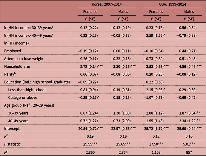
Model 3. Does the preponderance of 20- to 29-year-olds among never-married women explain the lack of a reverse gradient? Regression with interaction between age and household income
The results in the previous analysis found no detectable association between BMI and income in the never-married sample, as expected exclusively by the theory of anti-fat discrimination in marriage. However, the lack of effect among never-married women may have been due to the preponderance in that group of 20- to 29-year-olds who had not yet had sufficient exposure to deprivation or to labour market discrimination to create a reverse gradient. This concern rests on the assumption that the reverse gradient will become stronger with increasing age. To assess whether the reverse gradient becomes stronger among women with increasing age, a regression was run including an interaction term between age group and income for both never-married and currently-married women. Among currently-married women in both countries, there was no significant interaction between age and income, indicating that there was not an increasing association between household income and BMI with increasing age (p>0.10). Among never-married women in Korea, there was also no significant interaction between age and income (p>0.10). Among never-married women in the US, there was a significant interaction, with the BMI–income relationships differing between the 20–29 and 40–49 year age groups. However, it indicated that increasing age actually led to increasingly positive associations between BMI and household income, rather than an increasing reverse gradient (see Table 10). Thus, there is no evidence that the reverse gradient increases with increasing age.
Table 10. Estimated effects of income on BMI by age among never-married women, Korea (2007–2014) and USA (1999–2014)

a Reference group: 20s.
*p<0.05; **p<0.01; ***p<0.001; two tailed test; 95% Bonferroni adjusted confidence intervals (CIs) are reported; adjusted for sample weight.
Discussion
In nationally representative samples from two high-income countries with very different cultural backgrounds – South Korea (2007–2014) and the US (1999–2014) – this study demonstrated reverse gradients in BMI among women, but not men, confirming past findings about the gender-specificity of such reverse gradients (Sobal & Stunkard, Reference Sobal and Stunkard1989). Relevant to the explanations outlined in this article, the study also found that reverse gradients observed among women occurred exclusively among currently-married women, and not among never-married women. These findings are largely inconsistent with current deprivation theories that posit greater household incomes (regardless of marital status) should provide opportunities for consumption of costly, thinning foods or leisure exercise to meet thin body size ideals. They are also inconsistent with theories of anti-fat discrimination in the labour market, which would predict a negative correlation between household income and BMI regardless of marital status. On the other hand, the finding of reverse gradients exclusively among currently-married women is highly consistent with an explanation of these reverse gradients based on anti-fat discrimination in marriage, whereby women with higher BMIs are selected into lower-income households through marriage markets. These findings also point to the importance of going beyond including marital status as a simple covariate in analyses of income–obesity relationships (Pudrovska, Reference Pudrovska, Reither, Logan and Sherman-Wilkins2014), to including it as an interacting variable that can fundamentally alter the processes that lead to such gradients.
These findings are consistent with theories proposing that anti-fat discrimination in heterosexual marriage – rather than some generic effect of income on BMI or anti-fat discrimination in labour markets – is a key factor in creating the reverse gradient. It is not clear whether this sorting process occurs in low- and middle-income countries, but these findings and other evidence indicate that it does occur in high-income countries (Averett & Korenman, Reference Averett and Korenman1996; Mukhopadhyay, Reference Mukhopadhyay2008; Oreffice & Quintana-Domeque, Reference Oreffice and Quintana-Domeque2010; Chiappori et al., Reference Chiappori, Oreffice and Quintana-Domeque2012). Importantly, this anti-fat discrimination model does not require any individual capacity to lose weight – an assumption that is consistent with challenges most people face in controlling their body sizes (Kassirer & Angell, Reference Kassirer and Angell1998). Rather, it only requires that marriage markets sort existing variation in BMI into households according to household income.
Importantly, these analyses also ruled out a number of alternative hypotheses for the pattern. One possible alternative account for the lack of a reverse gradient among never-married women is the very young age distribution of never-married individuals in both countries. For example, about 82% of the sample of never-married Korean women were between 20 and 29 years of age, and 69% of the comparable US samples were in the same age group. If exposure to deprivation or anti-fat discrimination in labour markets only takes full effect in the 30s, then it is possible that the lack of a reverse gradient is due to the preponderance of 20- to 29-year-old never-married women in these samples. However, no evidence was found for a consistently increasing reverse gradient by age in any of the samples.
As stated in the Introduction, if the reverse gradient arises through differential selection in marriage markets, it is important to emphasize that this does not mean that women only prefer higher incomes in spouses and men only prefer thinner women in these samples. These are average results accounting for a population-level phenomenon in wealthy countries. Thus they gloss over substantial variation between individuals in their preferences and goals. Indeed, evidence from other studies of marital assortment indicates both women and men in the United States often prefer spouses with thinner bodies. Rather, the real asymmetry stems in quantitative (but not categorical) gender differences in concerns about spousal income (Averett & Korenman, Reference Averett and Korenman1996; Mukhopadhyay, Reference Mukhopadhyay2008; Oreffice & Quintana-Domeque, Reference Oreffice and Quintana-Domeque2010; Chiappori et al., Reference Chiappori, Oreffice and Quintana-Domeque2012). Nor do these associations necessarily reflect innate biological tendencies. Indeed, it is possible that any asymmetries in preferences emerge from an already-unequal system (McClintock, Reference McClintock2014). For example, men on average have access to higher salaries for the same effort in both South Korea and the US. It would be interesting to examine how a society’s gender equality in wages influences the reverse income–BMI gradient by changing the trade-offs in marriage markets. Specifically, if asymmetries in the labour market influence mate preferences, which in turn influence the income–BMI gradient, then it would be expected that countries with greater gender equality in income and in access to wage markets would have a weaker (or non-existent) reverse income–BMI gradient among women. Interestingly, across the two samples considered here, the opposite was found: a weaker gradient among South Korean married women despite a much larger pay gap (36.6% in South Korea compared with 17.9% in the US in 2013 according to the 2014 OECD).
There are a number of potential limitations to these analyses. The study focused on two forms of anti-fat discrimination – in labour markets and marriage – but other forms, such as discrimination in education, may also play a role in creating reverse BMI–income gradients (Han et al., Reference Han, Norton and Stearns2009, Reference Han, Norton and Powell2011; Pan et al., Reference Pan, Qin and Liu2012; Caliendo & Lee, Reference Caliendo and Lee2013; Mosca, Reference Mosca2013). Second, the study focused on BMI as a measure of obesity, as this is the standard tool used in the past to identify reverse gradients in obesity. However, it is well known that BMI confounds both fat mass and fat-free mass, so it is important to emphasize that any characterization of the reverse gradient in terms of BMI confounds both fat mass and fat-free mass (Hruschka et al., Reference Hruschka, Rush and Brewis2013; Hruschka & Hadley, Reference Hruschka and Hadley2016). The degree to which such reverse gradients reflect differences in fat mass versus fat-free mass also remains to be studied. For example, studies in both Germany and the United States that separate fat mass and lean mass indicate that in labour markets there is a wage penalty specifically for adiposity, whereas there is actually a slight wage premium for lean mass (e.g. more muscular individuals earn higher wages than their less muscular peers) (Wada & Tekin, Reference Wada and Tekin2010; Bozoyan & Wolbring, Reference Bozoyan and Wolbring2011). Finally, it is possible that there is no effect of household income on BMI among never-married women because they are less actively managing their weight than are currently-married women. However, this is unlikely in light of recent evidence from the NHANES study that never-married women are on average equally or more likely to be managing their weight than currently-married women, and that our own efforts to control for weight management in the current study did not alter the results (Klos & Sobal, Reference Klos and Sobal2013).
Finally, this study examined predicted cross-sectional patterns in observational data. Observational data, whether cross-sectional or longitudinal, are always open to inferential threats from omitted variables and alternative hypotheses. However, comparing contrasting predictions from a range of competing theories at least permits the comparison of those theories to establish which ones are most consistent with existing empirical data. In this case, predictions from theories of anti-fat discrimination in marriage were most consistent with the empirical patterns. However, it is possible that there are other better explanations that have not yet been proposed. An attempt was made to rule out three alternative explanations for the lack of association among never-married women – that they are less likely engage in weight management, that they have less time to translate income into weight reduction or that they are largely young women who have not yet been sufficiently exposed to deprivation or labour market discrimination. It is also possible that further refinements to deprivation theories can also account for the interaction with marital status. In such cases, future work examining ever-finer-grained data on the dynamics of marriage and weight changes in longitudinal data should provide new paths for comparing and testing such refinements. Despite these potential limitations, the current findings are most consistent with predictions of anti-fat discrimination in marriage. They also raise serious questions about the scope and generalizability of currently prevalent explanations for the reverse gradient based on deprivation or anti-fat discrimination in labour markets.
Funding
DJH acknowledges support from the National Science Foundation grant BCS-1658766, jointly funded by Programs in Cultural Anthropology and Methodology, Measurement and Statistics, and support from the Virginia G Piper Charitable Trust through an award to Mayo Clinic/ASU Obesity Solutions. The funder had no role in study design, data collection and analysis, decision to publish or preparation of the manuscript.
Conflicts of Interest
The authors report no conflicts of interest.
Ethical Approval
The analysis of secondary data from the US and Korean NHANES was approved by Arizona State University’s Institutional Review Board.


