


1. Introduction
Actuaries have produced forecasts of mortality since the beginning of the 20th century, in response to the adverse financial effects of mortality improvements over time on life annuities and pensions (Pollard, Reference Pollard1987). Thus, projected mortality tables for annuitants were one of the topics discussed at the 5th International Congress of Actuaries, Berlin, in 1906 (Cramér & Wold, Reference Cramér and Wold1935). Several authors have proposed new approaches for forecasting age-specific central mortality rates using statistical models (see Booth, Reference Booth2006; Booth & Tickle, Reference Booth and Tickle2008; Cairns et al., Reference Cairns, Blake and Dowd2008; Shang et al., Reference Shang, Booth and Hyndman2011, for reviews). Instead of modelling central mortality rates, we consider a compositional data analysis (CoDa) approach for modelling and forecasting the age-specific numbers of deaths in period life tables. Both central mortality rates or life-table death counts can be derived from the other based on standard life-table relations (for detail on the life table and its indicators, see Preston et al. (Reference Preston, Heuveline and Guillot2001), Chapter 3, or Dickson et al. (Reference Dickson, Hardy and Waters2009), Chapters 2–3). By using the life-table death distribution, we could model and forecast a redistribution of the density of life-table deaths, where deaths at younger ages are shifted towards older ages. Alternatively, we may consider a cohort life table that depicts the life history of a specific group of individuals but is dependent on projected mortality rates for those cohorts born more recently. Instead, we choose to study the period life table that represents the mortality conditions in a period of time (see also Oeppen, Reference Oeppen2008; Bergeron-Boucher et al., Reference Bergeron-Boucher, Canudas-Romo, Oeppen and Vaupel2017).
In the field of demography, Oeppen (Reference Oeppen2008) and Bergeron-Boucher et al. (Reference Bergeron-Boucher, Canudas-Romo, Oeppen and Vaupel2017) have put forward a principal component approach to forecast life-table death counts within a CoDa framework by considering age-specific life-table death count
 $(d_x)$
as compositional data. As with compositional data, the data are constrained to vary between two limits (e.g. 0 and a constant upper bound), which conditions their covariance structure. This feature can represent great advantages in a forecasting context (Lee, Reference Lee1998). Thus, Oeppen (Reference Oeppen2008) demonstrated that using CoDa to forecast age-specific mortality does not lead to more pessimistic results than forecasting age-specific mortality (see e.g. Wilmoth, Reference Wilmoth1995). Apart from providing an informative description of the mortality experience of a population, the age-at-death distribution yields readily available information on the “central longevity indicators” (e.g. mean, median and modal age at death, see Cheung et al., Reference Cheung, Robine, Tu and Caselli2005 and Canudas-Romo, Reference Canudas-Romo2010) as well as lifespan variability (e.g. Robine, Reference Robine2001; Vaupel et al., Reference Vaupel, Zhang and van Raalte2011; van Raalte & Caswell, Reference van Raalte and Caswell2013; van Raalte et al., Reference van Raalte, Martikainen and Myrskylä2014; Aburto & van Raalte, Reference Aburto and van Raalte2018).
$(d_x)$
as compositional data. As with compositional data, the data are constrained to vary between two limits (e.g. 0 and a constant upper bound), which conditions their covariance structure. This feature can represent great advantages in a forecasting context (Lee, Reference Lee1998). Thus, Oeppen (Reference Oeppen2008) demonstrated that using CoDa to forecast age-specific mortality does not lead to more pessimistic results than forecasting age-specific mortality (see e.g. Wilmoth, Reference Wilmoth1995). Apart from providing an informative description of the mortality experience of a population, the age-at-death distribution yields readily available information on the “central longevity indicators” (e.g. mean, median and modal age at death, see Cheung et al., Reference Cheung, Robine, Tu and Caselli2005 and Canudas-Romo, Reference Canudas-Romo2010) as well as lifespan variability (e.g. Robine, Reference Robine2001; Vaupel et al., Reference Vaupel, Zhang and van Raalte2011; van Raalte & Caswell, Reference van Raalte and Caswell2013; van Raalte et al., Reference van Raalte, Martikainen and Myrskylä2014; Aburto & van Raalte, Reference Aburto and van Raalte2018).
Compositional data arise in many other scientific fields, such as geology (geochemical elements), economics (income/expenditure distribution), medicine (body composition), food industry (food composition), chemistry (chemical composition), agriculture (nutrient balance bionomics), environmental sciences (soil contamination), ecology (abundance of different species) and demography (life-table death counts). In the field of statistics, Scealy et al. (Reference Scealy, de Caritat, Grunsky, Tsagris and Welsh2015) use CoDa to study the concentration of chemical elements in sediment or rock samples. Scealy & Welsh (Reference Scealy and Welsh2017) applied CoDa to analyse total weekly expenditure on food and housing costs for households in a chosen set of domains. Delicado (Reference Delicado2011) and Kokoszka et al. (Reference Kokoszka, Miao, Petersen and Shang2019) use CoDa to analyse density functions and implement dimension-reduction techniques on the constrained compositional data space.
Compositional data are defined as a random vector of K positive components
 $\textbf{{\textit{D}}} = [\textit{d}_1,\dots,d_K]$
with strictly positive values whose sum is a given constant, set typically equal to 1 (portions), 100 (%) and
$\textbf{{\textit{D}}} = [\textit{d}_1,\dots,d_K]$
with strictly positive values whose sum is a given constant, set typically equal to 1 (portions), 100 (%) and
 $10^6$
for parts per million (ppm) in geochemical trace element compositions (Aitchison, Reference Aitchison1986: 1). The sample space of compositional data is thus the simplex
$10^6$
for parts per million (ppm) in geochemical trace element compositions (Aitchison, Reference Aitchison1986: 1). The sample space of compositional data is thus the simplex
 \begin{equation*}
\mathcal{S}^K = \left\{\textbf{\textit{D}} = \left(d_1, \dots, d_K\right)^{\top}, \quad d_x>0, \quad \sum^K_{x=1}d_x = c\right\}
\end{equation*}
\begin{equation*}
\mathcal{S}^K = \left\{\textbf{\textit{D}} = \left(d_1, \dots, d_K\right)^{\top}, \quad d_x>0, \quad \sum^K_{x=1}d_x = c\right\}
\end{equation*}
where
 $\mathcal{S}$
denotes a simplex, c is a fixed constant, ┬ denotes vector transpose and the simplex sample space is a (K − 1)-dimensional subset of real-valued space
$\mathcal{S}$
denotes a simplex, c is a fixed constant, ┬ denotes vector transpose and the simplex sample space is a (K − 1)-dimensional subset of real-valued space
 $R^{K-1}$
.
$R^{K-1}$
.
Compositional data are subject to a sum constraint, which in turn imposes unpleasant constraints upon the variance–covariance structure of the raw data. The standard approach involves breaking the sum constraint using a transformation of the raw data to remove the constraint, before applying conventional statistical techniques to the transformed data. Among all possible transformations, the family of log-ratio transformations is commonly used. This family includes the additive log-ratio, the multiple log-ratio, the centred log-ratio transformations (Aitchison & Shen, Reference Aitchison and Shen1980; Aitchison, Reference Aitchison1982, Reference Aitchison1986) and the isometric log-ratio transformation (Egozcue et al., Reference Egozcue, Pawlowsky-Glahn, Mateu-Figueraz and Barceló-Vidal2003).
The contributions of this paper are threefold: First, as the CoDa framework of Oeppen (Reference Oeppen2008) is an adaptation of the Lee–Carter (LC) model to compositional data, our work could be seen as an adaptation of Hyndman & Ullah’s (Reference Hyndman and Ullah2007) to a CoDa framework. Second, we apply the CoDa method of Oeppen (Reference Oeppen2008) to model and forecast the age distribution of life-table death counts, from which we obtain age-specific survival probabilities, and we determine immediate temporary annuity prices. Third, we propose a nonparametric bootstrap method for constructing prediction intervals for the future age distribution of life-table death counts.
Using the Australian age- and sex-specific life-table death counts from 1921 to 2014, we evaluate and compare the 1- to 20-step-ahead point forecast accuracy and interval forecast accuracy among the CoDa, Hyndman–Ullah (HU) method, LC method and two naïve random walk methods. To evaluate point forecast accuracy, we use the mean absolute percentage error (MAPE). To assess interval forecast accuracy, we utilise the interval score of Gneiting & Raftery (Reference Gneiting and Raftery2007) and Gneiting & Katzfuss (Reference Gneiting and Katzfuss2014); see section 5.1 for details. Regarding both point forecast accuracy and interval forecast accuracy, the CoDa method performs the best overall among the three methods that we have considered. The improved forecast accuracy of life-table death counts is of great importance to actuaries for determining remaining life expectancies and pricing temporary annuities for various ages and maturities.
The remainder of this paper is organised as follows: section 2 describes the data set, obtained from the Human Mortality Database (2019), which is Australian age- and sex-specific life-table death counts from 1921 to 2014. Section 3 introduces the CoDa method for producing the point and interval forecasts of the age distribution of life-table death counts. Section 4 studies the goodness of fit of the CoDa method and provides an example for generating point and interval forecasts. Using the MAPE and mean interval score in section 5, we evaluate and compare the point and interval forecast accuracies among the methods considered. Section 6 applies the CoDa method to estimate the single-premium temporary immediate annuity prices for various ages and maturities for a female policyholder residing in Australia. Conclusions are presented in section 7, along with some reflections on how the methods presented here can be extended.
2. Australian Age- and Sex-Specific Life-Table Death Counts
We consider Australian age- and sex-specific life-table death counts from 1921 to 2014, obtained from the Human Mortality Database (2019). Although we use all data that include the first and second World War periods, a feature of our proposed method is to use an automatic algorithm of Hyndman & Khandakar (Reference Hyndman and Khandakar2008) to select the optimal data-driven parameters in exponential smoothing (ETS) forecasting method. As with ETS forecasting method, it assigns more weights to the recent data than distant past data. In practice, it is likely that only a few of the most distant past data may influence our forecasts, regardless of the starting point.
We study life-table death counts, where the life-table radix (i.e. a population experiencing 100,000 births annually) is fixed at 100,000 at age 0 for each year. For the life-table death counts, there are 111 ages, and these are age 0, 1, …, 109, 110+. Due to rounding, there are zero counts for age 110+ at some years. To rectify this problem, we prefer to use the probability of dying (i.e.
 $q_x$
) and the life-table radix to recalculate our estimated death counts (up to six decimal places). In doing so, we obtain more detailed death counts than the ones reported in the Human Mortality Database (2019).
$q_x$
) and the life-table radix to recalculate our estimated death counts (up to six decimal places). In doing so, we obtain more detailed death counts than the ones reported in the Human Mortality Database (2019).
To understand the principal features of the data, Figure 1 presents rainbow plots of the female and male age-specific life-table death counts in Australia from 1921 to 2014 in a single-year group. The time ordering of the curves follows the colour order of a rainbow, where data from the distant past are shown in red and the more recent data are shown in purple (see Hyndman & Shang, Reference Hyndman and Shang2010, for other examples). Both figures demonstrate a decreasing trend in infant death counts and a typical negatively skewed distribution for the life-table death counts, where the peaks shift to higher ages for both females and males. This shift is a primary source of the longevity risk, which is a major issue for insurers and pension funds, especially in the selling and risk management of annuity products (see Denuit et al., Reference Denuit, Devolder and Goderniaux2007, for a discussion). Moreover, the spread of the distribution indicates lifespan variability. A decrease in variability over time can be observed directly and can be measured, for example, with the interquartile range of life-table ages at death or the Gini coefficient (for comprehensive reviews, see Wilmoth & Horiuchi, Reference Wilmoth and Horiuchi1999; van Raalte & Caswell, Reference van Raalte and Caswell2013; Debón et al., Reference Debón, Chaves, Haberman and Villa2017). Age-at-death distributions thus provide critical insights on longevity and lifespan variability that cannot be grasped directly from either mortality rates or the survival function.
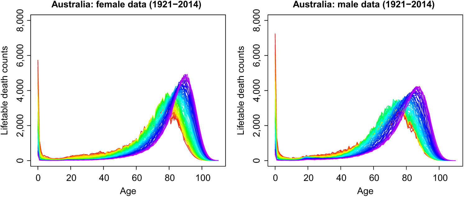
Figure 1. Rainbow plots of age-specific life-table death counts from 1921 to 2014 in a single-year group. The oldest years are shown in red, with the most recent years in violet. Curves are ordered chronologically according to the colours of the rainbow.
3. Forecasting Method
3.1 Compositional data analysis
In the field of demography, Oeppen (Reference Oeppen2008) and Bergeron-Boucher et al. (Reference Bergeron-Boucher, Canudas-Romo, Oeppen and Vaupel2017) have laid the foundations by presenting a modelling and forecasting framework. Following Oeppen (Reference Oeppen2008) and Bergeron-Boucher et al. (Reference Bergeron-Boucher, Canudas-Romo, Oeppen and Vaupel2017), a CoDa method can be summarised as follows:
(1) We begin from a data matrix
 $\textbf{\textit{D}}$
of size
$n\times K$
of the life-table death counts
$(d_{t,x})$
with n rows representing the number of years and K columns representing the age x. The sum of each row adds up to the life-table radix, such as 100,000. Since we are working with life-table death counts, it is not necessary to have population-at-risk estimates.
$\textbf{\textit{D}}$
of size
$n\times K$
of the life-table death counts
$(d_{t,x})$
with n rows representing the number of years and K columns representing the age x. The sum of each row adds up to the life-table radix, such as 100,000. Since we are working with life-table death counts, it is not necessary to have population-at-risk estimates.(2) We compute the geometric mean at each age, given by
(1)For a given year t, we divide
\begin{equation}
\alpha_x = \exp^{\frac{1}{n}\sum^n_{t=1}\ln (d_{t,x})}, \qquad x = 1,\dots, K,\quad t=1,\dots,n
\label{eqn1}
\end{equation}
$(d_{t,1},\dots,d_{t,K})$
by the corresponding geometric means
$(\alpha_1,\dots,\alpha_K)$
, and then standardise all elements so as to sum up to unity. As with compositional data, it is more important to know a relative proportion of each component (i.e. age) than the sum of all components. Although the life-table radix is 100,000 customarily, we model and forecast relative proportions, which are then multiplied by 100,000 to obtain forecast life-table death counts. Via standardisation, this is expressed as where
\begin{equation*}
f_{t,x} = \frac{d_{t,x}/\alpha_x}{\sum^K_{x=1}d_{t,x}/\alpha_x}
\end{equation*}
$f_{t,x}$
denotes de-centred data.(3) Log-ratio transformation. Aitchison (Reference Aitchison1982, Reference Aitchison1986) showed that compositional data are represented in a restricted space where the components can only vary between 0 and a positive constant. Therefore, Aitchison (Reference Aitchison1982, Reference Aitchison1986) proposed a log-ratio transformation to transform the data into a real-valued space. We apply the centred log-ratio transformation, given by
where
\begin{equation*}
z_{t,x} = \ln\left(\frac{f_{t,x}}{g_t}\right)
\end{equation*}
$g_t$
denotes the geometric mean over the age at time t, given byThe transformed data matrix is denoted as
\begin{equation*}
g_t = \exp^{\frac{1}{K}\sum^K_{x=1}\ln (f_{t,x})}
\end{equation*}
$\textbf{\textit{Z}}$
with elements
$z_{t,x}\in R$
, where R denotes real-valued space.(4) Principal component analysis. Principal component analysis is then applied to the matrix
$\textbf{\textit{Z}}$
, to obtain the estimated principal components and their scores,(2)where
\begin{equation}
z_{t,x} = \sum_{\ell=1}^{\min(n,K)}\widehat{\beta}_{t,\ell}\widehat{\phi}_{\ell,x} = \sum^L_{\ell=1}\widehat{\beta}_{t,\ell}\widehat{\phi}_{\ell,x}+\widehat{\varpi}_{t,x}
\label{eqn2}
\end{equation}
$\widehat{\varpi}_{t,x}$
denotes model residual term for age x in year t,
$\{\widehat{\phi}_{1,x},\dots,\widehat{\phi}_{L,x}\}$
represents the first L sets of estimated principal components,
$\{\widehat{\beta}_{t,1},\dots,\widehat{\beta}_{t,L}\}$
represents the first L sets of estimated principal component scores for time t and L denotes the number of retained principal components.(5) Forecast of principal component scores. Via a univariate time series forecasting method, such as ETS, we obtain the h-step-ahead forecast of the
$\ell^{\text{th}}$
principal component score
$\widehat{\beta}_{n+h, \ell}$
, where h denotes forecast horizon (see also Hyndman & Ullah, Reference Hyndman and Ullah2007). We utilise an automatic algorithm developed by Hyndman & Khandakar (Reference Hyndman and Khandakar2008) to determine the optimal ETS model based on the corrected Akaike information criterion (Hurvich & Tsai, Reference Hurvich and Tsai1993). Conditioning on the estimated principal components and observed data, the forecast of
$z_{n+h,x}$
can be obtained by(3)In (3), the principal component scores can be modelled and forecasted by an ETS method. To select the optimal ETS parameter, we use the automatic search algorithm of Hyndman & Khandakar (Reference Hyndman and Khandakar2008) by the smallest corrected Akaike information criterion. In Table 1, we also consider three other forecasting methods, namely autoregressive integrated moving average (ARIMA), random walk with drift (RWD) and random walk without drift (RW).
\begin{equation}
\skew2\widehat{z}_{n+h|n, x} = \sum^{L}_{\ell=1}\widehat{\beta}_{n+h|n,\ell}\widehat{\phi}_{\ell,x}
\label{eqn3}
\end{equation}
(6) Transform back to the compositional data. We take the inverse centred log-ratio transformation, given by
where
\begin{equation*}
\skew4\widehat{\textbf{\textit{f}}}_{n+h|n} = \left[\frac{\exp^{\skew2\widehat{z}_{n+h|n, 1}}}{\sum^K_{x=1}\exp^{\skew2\widehat{z}_{n+h|n, x}}}, \frac{\exp^{\skew2\widehat{z}_{n+h|n, 2}}}{\sum^K_{x=1}\exp^{\skew2\widehat{z}_{n+h|n, x}}}, \dots,\frac{\exp^{\skew2\widehat{z}_{n+h|n, K}}}{\sum^K_{x=1}\exp^{\skew2\widehat{z}_{n+h|n, x}}}\right]
\end{equation*}
$\skew2\widehat{z}_{n+h|n, x}$
denotes the forecasts in (3).(7) Finally, we add back the geometric means, to obtain the forecasts of the life-table death matrix
$d_{n+h}$
,where
\begin{align*}
\skew9\widehat{\textbf{\textit{d}}}_{n+h|n} &= \left[\frac{\skew4\widehat{f}_{n+h|n, 1}\times \alpha_1}{\sum^K_{x=1}\skew4\widehat{f}_{n+h|n, x}\times \alpha_x}, \frac{\skew4\widehat{f}_{n+h|n,2}\times \alpha_2}{\sum^K_{x=1}\skew4\widehat{f}_{n+h|n,x}\times \alpha_x},\dots,\frac{\skew4\widehat{f}_{n+h|n,K}\times \alpha_K}{\sum^K_{x=1}\skew4\widehat{f}_{n+h|n,x}\times \alpha_x}\right]
\end{align*}
$\alpha_x$
is the age-specific geometric mean given in (1).


Table 1. A comparison of the point and interval forecast accuracy, as measured by the overall MAPE and mean interval score, among the CoDa, HU, LC and two naïve RW methods (in italic) using the holdout sample of the Australian female and male data.
Note: Further, we consider four univariate time series forecasting methods for the CoDa and HU methods. In terms of interval forecast accuracy, we compare the finite-sample performance between the proposed bootstrap approach and an existing bootstrap approach of Bergeron-Boucher et al. (Reference Bergeron-Boucher, Canudas-Romo, Oeppen and Vaupel2017). The smallest errors are highlighted in bold.
To determine the number of components L in (2) and (3), we consider a criterion known as cumulative percentage of variance (CPV) – that is, we define the value of L as the minimum number of components that reaches a certain level of the proportion of total variance explained by the L leading components such that
 $$L = {\rm{ }}\mathop {{\rm{argmin}}}\limits_{_{L:L \ge 1}} \left\{ {\sum\limits_{\ell = \mathds{1}}^L {{{\hat \lambda }_\ell }} /\sum\limits_{\ell = 1}^n {{{\hat \lambda }_\ell }} {1_{\left\{ {{{\hat \lambda }_\ell } > 0} \right\}}} \ge \delta } \right\}$$
where
 $\delta = 85\%$
(see also Horváth & Kokoszka, Reference Horváth and Kokoszka2012, 41) and
$\delta = 85\%$
(see also Horváth & Kokoszka, Reference Horváth and Kokoszka2012, 41) and
 $\mathds{1}_{\{\cdot\}}$
denotes the binary indicator function that excludes possible zero eigenvalues. For the Australian female and male data, the chosen number of components is
$\mathds{1}_{\{\cdot\}}$
denotes the binary indicator function that excludes possible zero eigenvalues. For the Australian female and male data, the chosen number of components is
 $L=1$
and
$L=1$
and
 $L=2$
, respectively.
$L=2$
, respectively.
We highlight some similarities and differences between Oeppen’s (Reference Oeppen2008) approach and Lee & Carter’s (Reference Lee and Carter1992) approach. From Steps 3–5, Oeppen’s (Reference Oeppen2008) approach uses the Lee & Carter’s (Reference Lee and Carter1992) approach to model and forecast the log-ratio of life-table death counts. The difference is that the Oeppen’s (Reference Oeppen2008) approach works with life-table death counts in a constrained space, whereas the Lee & Carter’s (Reference Lee and Carter1992) approach works with real-valued log mortality rates.
When the number of components
 $L=1$
, our proposed CoDa method corresponds to the one presented by Oeppen (Reference Oeppen2008) and Bergeron-Boucher et al. (Reference Bergeron-Boucher, Canudas-Romo, Oeppen and Vaupel2017). However, we allow the possibility of using more than one pair of principal component and principal component scores in Steps 4 and 5. As a sensitivity analysis, we also consider setting the number of components to be
$L=1$
, our proposed CoDa method corresponds to the one presented by Oeppen (Reference Oeppen2008) and Bergeron-Boucher et al. (Reference Bergeron-Boucher, Canudas-Romo, Oeppen and Vaupel2017). However, we allow the possibility of using more than one pair of principal component and principal component scores in Steps 4 and 5. As a sensitivity analysis, we also consider setting the number of components to be
 $L=6$
(see also Hyndman & Booth, Reference Hyndman and Booth2008). From this aspect, our proposal shares some similarity with the Hyndman & Ullah’s (Reference Hyndman and Ullah2007) approach. The difference is that our proposal works with life-table death counts in a constrained space, whereas the Hyndman & Ullah’s (Reference Hyndman and Ullah2007) approach works with real-valued log mortality rates.
$L=6$
(see also Hyndman & Booth, Reference Hyndman and Booth2008). From this aspect, our proposal shares some similarity with the Hyndman & Ullah’s (Reference Hyndman and Ullah2007) approach. The difference is that our proposal works with life-table death counts in a constrained space, whereas the Hyndman & Ullah’s (Reference Hyndman and Ullah2007) approach works with real-valued log mortality rates.
3.2 Construction of prediction interval for the CoDa
Prediction intervals are a valuable tool for assessing the probabilistic uncertainty associated with point forecasts. The forecast uncertainty stems from both systematic deviations (e.g. due to parameter or model uncertainty) and random fluctuations (e.g. due to model error term). As was emphasised by Chatfield (Reference Chatfield1993, Reference Chatfield2000), it is essential to provide interval forecasts as well as point forecasts to
(1) assess future uncertainty levels;
(2) enable different strategies to be planned for a range of possible outcomes indicated by the interval forecasts;
(3) compare forecasts from different methods more thoroughly; and
(4) explore different scenarios based on various assumptions.
3.2.1 Proposed bootstrap method
We consider two sources of uncertainty: truncation errors in the principal component decomposition and forecast errors in the projected principal component scores. Since principal component scores are regarded as surrogates of the original functional time series, these principal component scores capture the temporal dependence structure inherited in the original functional time series (see also Salish & Gleim, Reference Salish and Gleim2015; Paparoditis, Reference Paparoditis2018; Shang, Reference Shang2018). By adequately bootstrapping the forecast principal component scores, we can generate a set of bootstrapped
 $\textbf{\textit{Z}}^*$
, conditional on the estimated mean function and estimated functional principal components from the observed Z in (3).
$\textbf{\textit{Z}}^*$
, conditional on the estimated mean function and estimated functional principal components from the observed Z in (3).
Using a univariate time series model, we can obtain multi-step-ahead forecasts for the principal component scores,
 $\{\widehat{\beta}_{1,\ell},\dots,\widehat{\beta}_{n,\ell}\}$
for
$\{\widehat{\beta}_{1,\ell},\dots,\widehat{\beta}_{n,\ell}\}$
for
 $l=1,\dots,L$
. Let the h-step-ahead forecast errors be given by
$l=1,\dots,L$
. Let the h-step-ahead forecast errors be given by
 $\widehat{\vartheta}_{t,h,\ell} = \widehat{\beta}_{t,\ell}-\widehat{\beta}_{t|t-h,\ell}$
for
$\widehat{\vartheta}_{t,h,\ell} = \widehat{\beta}_{t,\ell}-\widehat{\beta}_{t|t-h,\ell}$
for
 $t=h+1,\dots,n$
. These can then be sampled with replacement to give a bootstrap sample of
$t=h+1,\dots,n$
. These can then be sampled with replacement to give a bootstrap sample of
 $\beta_{n+h,\ell}$
:
$\beta_{n+h,\ell}$
:
 \begin{equation*}
\widehat{\beta\,}_{n+h|n,\ell}^{(b)} = \widehat{\beta}_{n+h|n,\ell}+\widehat{\vartheta}_{\ast, h, \ell}^{(b)}, \qquad b=1,\dots,B
\end{equation*}
\begin{equation*}
\widehat{\beta\,}_{n+h|n,\ell}^{(b)} = \widehat{\beta}_{n+h|n,\ell}+\widehat{\vartheta}_{\ast, h, \ell}^{(b)}, \qquad b=1,\dots,B
\end{equation*}
where
 $B=1,000$
symbolises the number of bootstrap replications and
$B=1,000$
symbolises the number of bootstrap replications and
 $\widehat{\vartheta}_{\ast, h, \ell}^{(b)}$
are sampled with replacement from
$\widehat{\vartheta}_{\ast, h, \ell}^{(b)}$
are sampled with replacement from
 $\{\widehat{\vartheta}_{t, h, \ell}\}$
.
$\{\widehat{\vartheta}_{t, h, \ell}\}$
.
Assuming the first L principal components approximate the data
 $\textbf{\textit{Z}}$
relatively well, the model residual should contribute nothing but random noise. Consequently, we can bootstrap the model fit errors in (2) by sampling with replacement from the model residual term
$\textbf{\textit{Z}}$
relatively well, the model residual should contribute nothing but random noise. Consequently, we can bootstrap the model fit errors in (2) by sampling with replacement from the model residual term
 $\{\widehat{\varpi}_{1,x},\dots,\widehat{\varpi}_{n,x}\}$
for a given age x.
$\{\widehat{\varpi}_{1,x},\dots,\widehat{\varpi}_{n,x}\}$
for a given age x.
Adding all two components of variability, we obtain B variants for
 $z_{n+h,x}$
,
$z_{n+h,x}$
,
 \begin{equation*}
\skew2\widehat{z\,\,}_{n+h|n,x}^{(b)} = \sum^L_{\ell=1}\widehat{\beta\,}^{(b)}_{n+h|n,\ell}\widehat{\phi}_{\ell,x}+\widehat{\varpi}_{n+h,x}^{(b)}
\end{equation*}
\begin{equation*}
\skew2\widehat{z\,\,}_{n+h|n,x}^{(b)} = \sum^L_{\ell=1}\widehat{\beta\,}^{(b)}_{n+h|n,\ell}\widehat{\phi}_{\ell,x}+\widehat{\varpi}_{n+h,x}^{(b)}
\end{equation*}
where
 $\widehat{\beta\,}^{(b)}_{n+h,\ell}$
denotes the forecast of the bootstrapped principal component scores. The construction of the bootstrap samples
$\widehat{\beta\,}^{(b)}_{n+h,\ell}$
denotes the forecast of the bootstrapped principal component scores. The construction of the bootstrap samples
 $\{\skew1\widehat{z\ }^{(1)}_{n+h|n, x}, \dots, \skew1\widehat{z\ }^{(B)}_{n+h|n,x}\}$
is in the same spirit as the construction of the bootstrap samples for the LC method in (5) and for the HU method in Hyndman & Shang (Reference Hyndman and Shang2010).
$\{\skew1\widehat{z\ }^{(1)}_{n+h|n, x}, \dots, \skew1\widehat{z\ }^{(B)}_{n+h|n,x}\}$
is in the same spirit as the construction of the bootstrap samples for the LC method in (5) and for the HU method in Hyndman & Shang (Reference Hyndman and Shang2010).
With the bootstrapped
 $\skew1\widehat{z}_{n+h|n,x}^{\ (b)}$
, we follow Steps 6 and 7 in section 3.1, in order to obtain the bootstrap forecasts of
$\skew1\widehat{z}_{n+h|n,x}^{\ (b)}$
, we follow Steps 6 and 7 in section 3.1, in order to obtain the bootstrap forecasts of
 $d_{n+h,x}$
. At the
$d_{n+h,x}$
. At the
 $100(1-\gamma)\%$
nominal coverage probability, the pointwise prediction intervals are obtained by taking
$100(1-\gamma)\%$
nominal coverage probability, the pointwise prediction intervals are obtained by taking
 $\gamma/2$
and
$\gamma/2$
and
 $1-\gamma/2$
quantiles based on
$1-\gamma/2$
quantiles based on
 $\{\skew1\widehat{d\,}_{n+h|n,x}^{(1)},\dots,\skew1\widehat{d\,}_{n+h|n,x}^{(B)}\}$
.
$\{\skew1\widehat{d\,}_{n+h|n,x}^{(1)},\dots,\skew1\widehat{d\,}_{n+h|n,x}^{(B)}\}$
.
3.2.2 Existing bootstrap method
The construction of the prediction interval for CoDa has also been considered by Bergeron-Boucher et al. (Reference Bergeron-Boucher, Canudas-Romo, Oeppen and Vaupel2017). After applying the centred log-ratio transformation, Bergeron-Boucher et al. (Reference Bergeron-Boucher, Canudas-Romo, Oeppen and Vaupel2017) fit a nonparametric model to estimate the regression mean and obtain the residual matrix, from which bootstrap residual matrices can be obtained by randomly sampling with replacement from the original residual matrix. With the bootstrapped residuals, they then add them to the estimated regression mean to form the bootstrapped data samples. With each replication of the bootstrapped data samples, one could then re-apply singular value decomposition to obtain the first set of principal component and its associated scores. With the bootstrapped first set of principal component scores, one could then extrapolate them to the future using a univariate time-series forecasting method. By multiplying the bootstrapped forecast of the principal component scores with the bootstrap principal component, bootstrap forecasts of life-table death counts can be obtained via back-transformation.
In Table 1, we compare the interval forecast accuracy, as measured by the mean interval score, between the two ways of constructing prediction intervals (as described in sections 3.2.1 and 3.2.2).
3.3 Other forecasting methods
3.3.1 LC method
As a comparison, we revisit Lee & Carter’s (Reference Lee and Carter1992) method. To stabilise the higher variance associated with mortality at advanced old ages, it is necessary to transform the raw data by taking the natural logarithm. For those missing death counts at advanced old ages, we use a simple linear interpolation method to approximate the missing values. We denote by
 $m_{t,x}$
the observed mortality rate at year t at age x calculated as the number of deaths in the calendar year t at age x, divided by the corresponding mid-year population aged x. The model structure is given by
$m_{t,x}$
the observed mortality rate at year t at age x calculated as the number of deaths in the calendar year t at age x, divided by the corresponding mid-year population aged x. The model structure is given by
 \begin{equation}
\ln (m_{t,x}) = a_x + b_x\kappa_t + \epsilon_{t,x}
\label{eqn4}
\end{equation}
\begin{equation}
\ln (m_{t,x}) = a_x + b_x\kappa_t + \epsilon_{t,x}
\label{eqn4}
\end{equation}
where
 $a_x$
denotes the age pattern of the log mortality rates averaged across years;
$a_x$
denotes the age pattern of the log mortality rates averaged across years;
 $b_x$
denotes the first principal component reflecting relative change in the log mortality rate at each age;
$b_x$
denotes the first principal component reflecting relative change in the log mortality rate at each age;
 $\kappa_t$
is the first set of principal component scores by year t and measures the general level of the log mortality rates; and
$\kappa_t$
is the first set of principal component scores by year t and measures the general level of the log mortality rates; and
 $\epsilon_{t,x}$
denotes the residual at year t and age x.
$\epsilon_{t,x}$
denotes the residual at year t and age x.
The LC model in (4) is over-parametrised in the sense that the model structure is invariant under the following transformations:
 \begin{align*}
\{a_x, b_x, \kappa_t\} &\mapsto \{a_x, b_x/c, c\kappa_t\} \\
\{a_x, b_x, \kappa_t\} &\mapsto \{a_x-cb_x, b_x, \kappa_t+c\}
\end{align*}
\begin{align*}
\{a_x, b_x, \kappa_t\} &\mapsto \{a_x, b_x/c, c\kappa_t\} \\
\{a_x, b_x, \kappa_t\} &\mapsto \{a_x-cb_x, b_x, \kappa_t+c\}
\end{align*}
To ensure the model’s identifiability, Lee & Carter (Reference Lee and Carter1992) imposed two constraints, given as
 \begin{equation*}
\sum^n_{t=1}\kappa_t=0, \qquad \sum^{x_p}_{x=x_1}b_x=1
\end{equation*}
\begin{equation*}
\sum^n_{t=1}\kappa_t=0, \qquad \sum^{x_p}_{x=x_1}b_x=1
\end{equation*}
where n is the number of years, and p is the number of ages in the observed data set.
Also, the LC method adjusts
 $\kappa_t$
by refitting to the total number of deaths. This adjustment gives more weight to high rates, thus roughly counterbalancing the effect of using a log transformation of the mortality rates. The adjusted
$\kappa_t$
by refitting to the total number of deaths. This adjustment gives more weight to high rates, thus roughly counterbalancing the effect of using a log transformation of the mortality rates. The adjusted
 $k_{t}$
is then extrapolated using RW models. Lee & Carter (Reference Lee and Carter1992) used an RWD model, which can be expressed as
$k_{t}$
is then extrapolated using RW models. Lee & Carter (Reference Lee and Carter1992) used an RWD model, which can be expressed as
 \begin{equation*}
\kappa_{t}=\kappa_{t-1}+d+e_{t}
\end{equation*}
\begin{equation*}
\kappa_{t}=\kappa_{t-1}+d+e_{t}
\end{equation*}
where d is known as the drift parameter and measures the average annual change in the series, and
 $e_{t}$
is an uncorrelated error. It is notable that the RWD provides satisfactory results in many cases (see e.g. Tulkapurkar et al., Reference Tulkapurkar, Li and Boe2000; Lee & Miller, Reference Lee and Miller2001). From this forecast of the principal component scores, the forecast age-specific log mortality rates are obtained using the estimated age effects
$e_{t}$
is an uncorrelated error. It is notable that the RWD provides satisfactory results in many cases (see e.g. Tulkapurkar et al., Reference Tulkapurkar, Li and Boe2000; Lee & Miller, Reference Lee and Miller2001). From this forecast of the principal component scores, the forecast age-specific log mortality rates are obtained using the estimated age effects
 $a_x$
and
$a_x$
and
 $b_x$
in (4).
$b_x$
in (4).
Note that the LC model can also be formulated within a Generalised Linear Model framework with a generalised error distribution (see e.g. Tabeau, Reference Tabeau, Tabeau, Van Den Berg Jeths and Heathcote2001; Brouhns et al., Reference Brouhns, Denuit and Vermunt2002; Renshaw & Haberman, Reference Renshaw and Haberman2003). In this setting, the LC model parameters can be estimated by maximum likelihood methods based on the choice of the error distribution. Thus, in line with traditional actuarial practice, this approach assumes that the age- and period-specific number of deaths are independent realisations from a Poisson distribution. In the case of Gaussian error, the estimation method based on either the singular value decomposition or maximum likelihood method leads to the same parameter estimates.
Two sources of uncertainty are considered in the LC model: errors in the parameter estimation of the LC model and forecast errors in the forecasted principal component scores. Using a univariate time series model, we can obtain multi-step-ahead forecasts for the principal component scores,
 $\{\widehat{\kappa}_1,\dots,\widehat{\kappa}_n\}$
. Let the h-step-ahead forecast errors be given by
$\{\widehat{\kappa}_1,\dots,\widehat{\kappa}_n\}$
. Let the h-step-ahead forecast errors be given by
 $\nu_{t,h}=\widehat{\kappa}_t-\widehat{\kappa}_{t|t-h}$
for
$\nu_{t,h}=\widehat{\kappa}_t-\widehat{\kappa}_{t|t-h}$
for
 $t=h+1,\dots,n$
. These can then be sampled with replacement to give a bootstrap sample of
$t=h+1,\dots,n$
. These can then be sampled with replacement to give a bootstrap sample of
 $\kappa_{n+h}$
:
$\kappa_{n+h}$
:
 \begin{equation*}
\widehat{\kappa}_{n+h|n}^{(b)} = \widehat{\kappa}_{n+h|n}+\widehat{\nu}_{\ast,h}^{(b)},\qquad b=1,\dots,B
\end{equation*}
\begin{equation*}
\widehat{\kappa}_{n+h|n}^{(b)} = \widehat{\kappa}_{n+h|n}+\widehat{\nu}_{\ast,h}^{(b)},\qquad b=1,\dots,B
\end{equation*}
where
 $\widehat{\nu}_{\ast,h}^{(b)}$
are sampled with replacement from
$\widehat{\nu}_{\ast,h}^{(b)}$
are sampled with replacement from
 $\{\widehat{\nu}_{t,h}\}$
.
$\{\widehat{\nu}_{t,h}\}$
.
Assuming the first principal component approximates the data
 $\ln \textbf{\textit{m}}$
relatively well, the model residual should contribute nothing but random noise. Consequently, we can bootstrap the model fit error in (4) by sampling with replacement from the model residual term
$\ln \textbf{\textit{m}}$
relatively well, the model residual should contribute nothing but random noise. Consequently, we can bootstrap the model fit error in (4) by sampling with replacement from the model residual term
 $\{\,\widehat{e}_{1,x},\dots,\widehat{e}_{n,x}\}$
for a given age x.
$\{\,\widehat{e}_{1,x},\dots,\widehat{e}_{n,x}\}$
for a given age x.
Adding the two components of variability, we obtain B variants of
 $\ln m_{n+h,x}$
:
$\ln m_{n+h,x}$
:
 \begin{equation}
\ln \widehat{m}_{n+h|n,x}^{(b)} = \widehat{\kappa}_{n+h|n}^{\,(b)}\widehat{b}_x + \widehat{e}_{n+h,x}^{\,(b)}
\label{eqn5}
\end{equation}
\begin{equation}
\ln \widehat{m}_{n+h|n,x}^{(b)} = \widehat{\kappa}_{n+h|n}^{\,(b)}\widehat{b}_x + \widehat{e}_{n+h,x}^{\,(b)}
\label{eqn5}
\end{equation}
where
 $\widehat{\kappa}_{n+h|n}^{(b)}$
denotes the forecast of the bootstrapped principal component scores.
$\widehat{\kappa}_{n+h|n}^{(b)}$
denotes the forecast of the bootstrapped principal component scores.
Since the LC model forecasts age-specific central mortality rate, we convert forecast mortality rate to the probability of dying via a simple approximation. The formula is given as
 \begin{equation*}
\widehat{q}_{n+h|n,x} = 1 - \exp^{-\widehat{m}_{n+h|n,x}}
\end{equation*}
\begin{equation*}
\widehat{q}_{n+h|n,x} = 1 - \exp^{-\widehat{m}_{n+h|n,x}}
\end{equation*}
where
 $\widehat{q}_{n+h|n,x}$
denotes the probability of dying in age x and year
$\widehat{q}_{n+h|n,x}$
denotes the probability of dying in age x and year
 $n+h$
, and
$n+h$
, and
 $\widehat{m}_{n+h|n,x}$
denotes the forecast of central mortality rate in age x and year
$\widehat{m}_{n+h|n,x}$
denotes the forecast of central mortality rate in age x and year
 $n+h$
. With an initial life-table death count of 100,000, the forecast of
$n+h$
. With an initial life-table death count of 100,000, the forecast of
 $\skew1\widehat{d}_{n+h|n,x}$
can be obtained from
$\skew1\widehat{d}_{n+h|n,x}$
can be obtained from
 $\widehat{q}_{n+h|n,x}$
.
$\widehat{q}_{n+h|n,x}$
.
3.3.2 HU method
The HU method differs from the LC method in the following three aspects:
(1) Instead of modelling the original mortality rates, the HU method uses a P-spline with a monotonic constraint to smooth log mortality rates.
(2) Instead of using only one principal component and its associated scores, the HU method uses six sets of principal components and their scores.
(3) Instead of forecasting each set of principal component scores by an RWD method, the HU method uses an automatic algorithm of Hyndman & Khandakar (Reference Hyndman and Khandakar2008) to select the optimal model and estimate the parameters in a univariate time series forecasting method.
3.3.3 Random walk with and without drift
Given the findings of linear life expectancy (White, Reference White2002; Oeppen & Vaupel, Reference Oeppen and Vaupel2002) and the debate about its continuation (Bengtsson, Reference Bengtsson, Bengtsson and Keilman2003; Lee, Reference Lee2003), it is pertinent to compare the forecast accuracy of the CoDa method with a linear extrapolation method (see Alho & Spencer, Reference Alho and Spencer2005, 274–276 for an introduction). Using the centred log-ratio transformation, the linear extrapolation of
 $z_{t, x}$
in (2) is achieved by applying the RW and RWD models for each age:
$z_{t, x}$
in (2) is achieved by applying the RW and RWD models for each age:
 \begin{equation}
z_{t+1,x} =\zeta + z_{t,x} + e_{t+1,x}
\label{eqn6}
\end{equation}
\begin{equation}
z_{t+1,x} =\zeta + z_{t,x} + e_{t+1,x}
\label{eqn6}
\end{equation}
where
 $z_{t,x}$
represents the centred log ratio transformed data at age
$z_{t,x}$
represents the centred log ratio transformed data at age
 $x=0, 1, \dots, p$
in year
$x=0, 1, \dots, p$
in year
 $t=1,2,\dots,n-1$
,
$t=1,2,\dots,n-1$
,
 $\zeta$
denotes the drift term and
$\zeta$
denotes the drift term and
 $e_{t+1,x}$
denotes model error term. The h-step-ahead point and interval forecasts are given by
$e_{t+1,x}$
denotes model error term. The h-step-ahead point and interval forecasts are given by
 \begin{align}
\skew2\widehat{z}_{n+h|n,x} &= \text{E}\left[z_{n+h,x}|z_{1,x},\dots,z_{n,x}\right] = \zeta h + z_{n,x} \notag\\
\text{var}(\skew2\widehat{z}_{n+h|n,x}) &= \text{var}[z_{n+h,x}|z_{1,x},\dots,z_{n,x}] = \text{var}(z_{n,x}) + \text{var}(e_{n+h,x})
\label{eqn7}\end{align}
\begin{align}
\skew2\widehat{z}_{n+h|n,x} &= \text{E}\left[z_{n+h,x}|z_{1,x},\dots,z_{n,x}\right] = \zeta h + z_{n,x} \notag\\
\text{var}(\skew2\widehat{z}_{n+h|n,x}) &= \text{var}[z_{n+h,x}|z_{1,x},\dots,z_{n,x}] = \text{var}(z_{n,x}) + \text{var}(e_{n+h,x})
\label{eqn7}\end{align}
Based on (6) and (7), the RW can be obtained by omitting the drift term. Computationally, the forecasts of the RW and RWD are obtained by the rwf function in the forecast package (Hyndman et al., Reference Hyndman, Athanasopoulos, Bergmeir, Caceres, Chhay, O’Hara-Wild, Petropoulos, Razbash, Wang, Yasmeen, Team, Ihaka, Reid, Shaub, Tang and Zhou2019) in R (R Core Team, 2019). Then, by way of the back-transformation of the centred log ratio, naïve forecasts of age-specific life-table death counts can be obtained.
4. CoDa Model Fitting
For the life-table death counts, we examine the goodness of fit of the CoDa model to the observed data. The number of retained components L in (2) and (3) is determined by explaining at least 85% of the total variation. For the Australian female and male data, the chosen number of components is
 $L=1$
and
$L=1$
and
 $L=2$
, respectively. We attempt to interpret the first component for the Australian female and male age-specific life-table death counts.
$L=2$
, respectively. We attempt to interpret the first component for the Australian female and male age-specific life-table death counts.
Based on the historical death counts from 1921 to 2014 (i.e. 94 observations), in Figure 2, we present the geometric mean of female and male life-table death counts, given by
 $\alpha_x$
, transformed data matrix
$\alpha_x$
, transformed data matrix
 $\textbf{\textit{Z}}$
, and the first set of estimated principal component obtained by applying the principal component analysis to
$\textbf{\textit{Z}}$
, and the first set of estimated principal component obtained by applying the principal component analysis to
 $\textbf{\textit{Z}}$
. The shape of the first estimated principal component appears to be similar to the first estimated principal component in the Lee & Carter’s (Reference Lee and Carter1992) and Hyndman & Ullah’s (Reference Hyndman and Ullah2007) methods. Because
$\textbf{\textit{Z}}$
. The shape of the first estimated principal component appears to be similar to the first estimated principal component in the Lee & Carter’s (Reference Lee and Carter1992) and Hyndman & Ullah’s (Reference Hyndman and Ullah2007) methods. Because
 $\textbf{\textit{Z}}$
is unbounded, the principal component analysis captures a similar projection direction. By using the automatic ETS forecasting method, we produce the 20-step-ahead forecast of principal component scores for the year between 2015 and 2034.
$\textbf{\textit{Z}}$
is unbounded, the principal component analysis captures a similar projection direction. By using the automatic ETS forecasting method, we produce the 20-step-ahead forecast of principal component scores for the year between 2015 and 2034.

Figure 2. Elements of the CoDa method for analysing the female and male age-specific life-table death counts in Australia. We present the first principal component and its scores, although we use
 $L=6$
for fitting.
$L=6$
for fitting.
Apart from the graphical display, we measure the in-sample goodness of fit via an
 $R^2$
criterion given as
$R^2$
criterion given as
 \begin{equation*}
R^2 = 1- \frac{\sum^{111}_{x=1}\sum^{94}_{t=1}\left(d_{t,x} - \skew4\widehat{d}_{t,x}\right)^2}{\sum^{111}_{x=1}\sum^{94}_{t=1}\left(d_{t,x} - \overline{d}_x\right)^2}
\end{equation*}
\begin{equation*}
R^2 = 1- \frac{\sum^{111}_{x=1}\sum^{94}_{t=1}\left(d_{t,x} - \skew4\widehat{d}_{t,x}\right)^2}{\sum^{111}_{x=1}\sum^{94}_{t=1}\left(d_{t,x} - \overline{d}_x\right)^2}
\end{equation*}
where
 $d_{t,x}$
denotes the observed age-specific life-table death count for age x in year t and
$d_{t,x}$
denotes the observed age-specific life-table death count for age x in year t and
 $\skew4\widehat{d}_{t,x}$
denotes the fitted age-specific life-table death count obtained from the CoDa model. For the Australian female and male data, the
$\skew4\widehat{d}_{t,x}$
denotes the fitted age-specific life-table death count obtained from the CoDa model. For the Australian female and male data, the
 $R^2$
values are 0.9946 and 0.9899 using the CPV criterion while the
$R^2$
values are 0.9946 and 0.9899 using the CPV criterion while the
 $R^2$
values are 0.9987 and 0.9987 based on
$R^2$
values are 0.9987 and 0.9987 based on
 $L=6$
, respectively. Using the CPV criterion, we select
$L=6$
, respectively. Using the CPV criterion, we select
 $L=1$
for both female and male data. One remark is that choosing the number of principal components
$L=1$
for both female and male data. One remark is that choosing the number of principal components
 $L=6$
does not improve greatly the
$L=6$
does not improve greatly the
 $R^2$
values, but it improves the forecast accuracy greatly as will be shown in Table 1.
$R^2$
values, but it improves the forecast accuracy greatly as will be shown in Table 1.
5. Comparisons of Point and Interval Forecast Accuracy
5.1 Forecast error criteria
An expanding window analysis of a time-series model is commonly used to assess model and parameter stability over time, and prediction accuracy. The expanding window analysis determines the constancy of a model’s parameter by computing parameter estimates and their resultant forecasts over an expanding window of a fixed size through the sample (for details, Zivot & Wang, Reference Zivot and Wang2006: 313–314). Using the first 74 observations from 1921 to 1994 in the Australian female and male age-specific life-table death counts, we produce 1- to 20-step-ahead forecasts. Through an expanding-window approach, we re-estimate the parameters in the time series forecasting models using the first 75 observations from 1921 to 1995. Forecasts from the estimated models are then produced for 1- to 19-step-ahead points and intervals. We iterate this process by increasing the sample size by 1 year until reaching the end of the data period in 2014. This process produces 20 one-step-ahead forecasts, 19 two-step-ahead forecasts, …, and one 20-step-ahead forecast. We compare these forecasts with the holdout samples to determine the out-of-sample point forecast accuracy.
To evaluate the point forecast accuracy, we consider the MAPE that measures how close the forecasts are in comparison to the actual values of the variable being forecast, regardless of the direction of forecast errors. The error measure can be written as
 \begin{equation*}
\text{MAPE}(h) = \frac{1}{111\times (21-h)}\sum^{20}_{\varsigma=h}\sum^{111}_{x=1}\left|\frac{d_{n+\varsigma, x}-\skew4\widehat{d}_{n+\varsigma,x}}{d_{n+\varsigma, x}}\right|\times 100
\end{equation*}
\begin{equation*}
\text{MAPE}(h) = \frac{1}{111\times (21-h)}\sum^{20}_{\varsigma=h}\sum^{111}_{x=1}\left|\frac{d_{n+\varsigma, x}-\skew4\widehat{d}_{n+\varsigma,x}}{d_{n+\varsigma, x}}\right|\times 100
\end{equation*}
where
 $d_{n+\varsigma,x}$
denotes the actual holdout sample for the
$d_{n+\varsigma,x}$
denotes the actual holdout sample for the
 $x^{\text{th}}$
age and
$x^{\text{th}}$
age and
 $\varsigma^{\text{th}}$
forecasting year, while
$\varsigma^{\text{th}}$
forecasting year, while
 $\skew4\widehat{d}_{n+\varsigma,x}$
denotes the point forecasts for the holdout sample.
$\skew4\widehat{d}_{n+\varsigma,x}$
denotes the point forecasts for the holdout sample.
To evaluate and compare the interval forecast accuracy, we consider the interval score of Gneiting & Raftery (Reference Gneiting and Raftery2007). For each year in the forecasting period, the h-step-ahead prediction intervals are calculated at the
 $100(1-\gamma)\%$
nominal coverage probability. We consider the common case of the symmetric
$100(1-\gamma)\%$
nominal coverage probability. We consider the common case of the symmetric
 $100(1-\gamma)\%$
prediction intervals, with lower and upper bounds that are predictive quantiles at
$100(1-\gamma)\%$
prediction intervals, with lower and upper bounds that are predictive quantiles at
 $\gamma/2$
and
$\gamma/2$
and
 $1-\gamma/2$
, denoted by
$1-\gamma/2$
, denoted by
 $\skew4\widehat{d}^l_{n+\varsigma, x}$
and
$\skew4\widehat{d}^l_{n+\varsigma, x}$
and
 $\skew1\widehat{d}^u_{n+\varsigma, x}$
. As defined by Gneiting & Raftery (Reference Gneiting and Raftery2007), a scoring rule for the interval forecasts at time point
$\skew1\widehat{d}^u_{n+\varsigma, x}$
. As defined by Gneiting & Raftery (Reference Gneiting and Raftery2007), a scoring rule for the interval forecasts at time point
 $d_{n+\varsigma,x}$
is
$d_{n+\varsigma,x}$
is
 \begin{array}{*{20}{c}}
{{S_{\gamma ,\varsigma }}\left[ {\hat d_{n + \varsigma ,x}^l,\hat d_{n + \varsigma ,x}^u,{d_{n + \varsigma ,x}}} \right] = \left( {\hat d_{n + \varsigma ,x}^u - \hat d_{n + \varsigma ,x}^l} \right)} & { + \frac{2}{\gamma }\left( {\hat d_{n + \varsigma ,x}^l - {d_{n + \varsigma ,x}}} \right)\mathds{1}\left\{ {{d_{n + \varsigma ,x}} < \hat d_{n + \varsigma ,x}^l} \right\}} \\
{} & { + \frac{2}{\gamma }\left( {{d_{n + \varsigma ,x}} - \hat d_{n + \varsigma ,x}^u} \right)\mathds{1}\left\{ {{d_{n + \varsigma ,x}} > \hat d_{n + \varsigma ,x}^u} \right\}} \\
\end{array}
\begin{array}{*{20}{c}}
{{S_{\gamma ,\varsigma }}\left[ {\hat d_{n + \varsigma ,x}^l,\hat d_{n + \varsigma ,x}^u,{d_{n + \varsigma ,x}}} \right] = \left( {\hat d_{n + \varsigma ,x}^u - \hat d_{n + \varsigma ,x}^l} \right)} & { + \frac{2}{\gamma }\left( {\hat d_{n + \varsigma ,x}^l - {d_{n + \varsigma ,x}}} \right)\mathds{1}\left\{ {{d_{n + \varsigma ,x}} < \hat d_{n + \varsigma ,x}^l} \right\}} \\
{} & { + \frac{2}{\gamma }\left( {{d_{n + \varsigma ,x}} - \hat d_{n + \varsigma ,x}^u} \right)\mathds{1}\left\{ {{d_{n + \varsigma ,x}} > \hat d_{n + \varsigma ,x}^u} \right\}} \\
\end{array}
where
 $\mathds{1}\{\cdot\}$
represents the binary indicator function and
$\mathds{1}\{\cdot\}$
represents the binary indicator function and
 $\gamma$
denotes the level of significance, customarily
$\gamma$
denotes the level of significance, customarily
 $\gamma=0.2$
or
$\gamma=0.2$
or
 $\gamma=0.05$
. The interval score rewards a narrow prediction interval, if and only if the true observation lies within the prediction interval. The optimal interval score is achieved when
$\gamma=0.05$
. The interval score rewards a narrow prediction interval, if and only if the true observation lies within the prediction interval. The optimal interval score is achieved when
 $d_{n+\varsigma, x}$
lies between
$d_{n+\varsigma, x}$
lies between
 $\widehat{d}_{n+\varsigma,x}^l$
and
$\widehat{d}_{n+\varsigma,x}^l$
and
 $\widehat{d}_{n+\varsigma, x}^u$
, and the distance between
$\widehat{d}_{n+\varsigma, x}^u$
, and the distance between
 $\widehat{d}_{n+\varsigma, x}^l$
and
$\widehat{d}_{n+\varsigma, x}^l$
and
 $\widehat{d}_{n+\varsigma, x}^u$
is minimal.
$\widehat{d}_{n+\varsigma, x}^u$
is minimal.
For different ages and years in the forecasting period, the mean interval score is defined by
 \begin{equation*}
\overline{S}_{\gamma}(h) = \frac{1}{111\times (21-h)} \sum_{\varsigma = h}^{20} \sum_{x=1}^{111} S_{\gamma,\varsigma}\left[\widehat{d}_{n+\varsigma,x}^{l}, \widehat{d}_{n+\varsigma,x}^{u}; d_{n+\varsigma,x}\right]
\end{equation*}
\begin{equation*}
\overline{S}_{\gamma}(h) = \frac{1}{111\times (21-h)} \sum_{\varsigma = h}^{20} \sum_{x=1}^{111} S_{\gamma,\varsigma}\left[\widehat{d}_{n+\varsigma,x}^{l}, \widehat{d}_{n+\varsigma,x}^{u}; d_{n+\varsigma,x}\right]
\end{equation*}
where
 $S_{\gamma,\varsigma}\left[\widehat{d}_{n+\varsigma,x}^{l}, \widehat{d}_{n+\varsigma,x}^{u}; d_{n+\varsigma,x}\right]$
denotes the interval score at the
$S_{\gamma,\varsigma}\left[\widehat{d}_{n+\varsigma,x}^{l}, \widehat{d}_{n+\varsigma,x}^{u}; d_{n+\varsigma,x}\right]$
denotes the interval score at the
 $\varsigma^{\text{th}}$
curve in the forecasting year.
$\varsigma^{\text{th}}$
curve in the forecasting year.
5.2 Forecast results
Using the expanding window approach, we compare the point and interval forecast accuracies among the CoDa, HU, LC and two naïve RW methods based on the MAPE and mean interval score. Also, we consider forecasting each set of the estimated principal component scores by the ARIMA, ETS, RWD and RW. The overall point and interval forecast error results are presented in Table 1, where we average over the 20 forecast horizons. From Table 1, we find that the CoDa method with the ETS forecasting method generally performs the best among a range of methods considered. Among the four univariate time series forecasting methods, the ETS method produces the smallest errors and thus is recommended to be used in practice. Also, setting
 $L=6$
, including additional principal component decomposition pairs, generally provides more accurate point and interval forecast accuracies than setting
$L=6$
, including additional principal component decomposition pairs, generally provides more accurate point and interval forecast accuracies than setting
 $L=1$
or
$L=1$
or
 $L=2$
for the Australian female and male data.
$L=2$
for the Australian female and male data.
The CoDa method tends to provide less bias forecasts than the LC method as it allows the rate of mortality improvements to change over time (see Bergeron-Boucher et al., Reference Bergeron-Boucher, Canudas-Romo, Oeppen and Vaupel2017). With respect to the positivity and summability constraints, the CoDa method can adopt temporal changes of the age distribution of the life-table death counts over the years. The unsatisfactory performance of the HU and LC methods may be because of the approximation of converting the forecasts of central mortality rate to the probability of dying at higher ages. The inferior performance of the two naïve RW methods may be because of their slow responses to adapt to the change of age distribution of death counts. Between the two naïve RW methods, we found that the RW is preferable for producing point forecasts, while the RWD is preferable for producing interval forecasts.
While Table 1 presents the average over 20 forecast horizons, we show the 1-step-ahead to 20-step-ahead point and interval forecast errors in Figure 3. Since it is advantageous to set
 $L=6$
, we report the CoDa method with the ETS forecasting method and
$L=6$
, we report the CoDa method with the ETS forecasting method and
 $L=6$
in Figure 3. The difference in forecast accuracy between the CoDa and the other methods is widening over the forecast horizon. We suspect that in the relatively longer forecast horizon, the errors associated with all the methods become larger, but they are relatively smaller for the CoDa method with the ETS forecasting method and
$L=6$
in Figure 3. The difference in forecast accuracy between the CoDa and the other methods is widening over the forecast horizon. We suspect that in the relatively longer forecast horizon, the errors associated with all the methods become larger, but they are relatively smaller for the CoDa method with the ETS forecasting method and
 $L=6$
.
$L=6$
.

Figure 3. A comparison of the point and interval forecast accuracy, as measured by the MAPE and mean interval score, among the CoDa, HU, LC and two naïve RW methods using the holdout sample of the Australian female and male data. In the CoDa method, we use the ETS forecasting method with the number of principal components
 $L=6$
.
$L=6$
.
6. Application to a Single-Premium Temporary Immediate Annuity
An important use of mortality forecasts for those individuals at ages over 60 is in the pension and insurance industries, whose profitability and solvency crucially rely on accurate mortality forecasts to appropriately hedge longevity risks. When a person retires, an optimal way of guaranteeing one individual’s financial income in retirement is to purchase an annuity (as demonstrated by Yaari, Reference Yaari1965). An annuity is a financial contract offered by insurers guaranteeing a steady stream of payments for either a temporary or the lifetime of the annuitants in exchange for an initial premium fee.
Following Shang & Haberman (Reference Shang and Haberman2017), we consider temporary annuities, which have grown in popularity in a number of countries (e.g. Australia and the USA), because lifetime immediate annuities, where rates are locked in for life, have been shown to deliver poor value for money (i.e. they may be expensive for the purchasers; see e.g. Cannon & Tonks, Reference Cannon and Tonks2008, Chapter 6). These temporary annuities pay a pre-determined and guaranteed level of income that is higher than the level of income provided by a lifetime annuity for a similar premium. Fixed-term annuities offer an alternative to lifetime annuities and allow the purchaser the option of also buying a deferred annuity at a later date.
Using the CoDa method, we obtain forecasts of age-specific life-table death counts and then determine the corresponding survival probabilities. In Figure 4, we present the age-specific life-table death count forecasts from 2015 to 2064 for Australian females.

Figure 4. Age-specific life-table death count forecasts from 2015 to 2064 for Australian females.
With the mortality forecasts, we then input the forecasts of death counts to the calculation of single-premium term immediate annuities (see Dickson et al., Reference Dickson, Hardy and Waters2009: 114), and we adopt a cohort approach to the calculation of the survival probabilities. The
 $\tau$
year survival probability of a person aged x currently at
$\tau$
year survival probability of a person aged x currently at
 $t=0$
(or year 2016) is determined by
$t=0$
(or year 2016) is determined by
 \begin{align*}
_{\tau}p_x = \prod^{\tau}_{j=1} p_{x+j-1}
=\prod^{\tau}_{j=1} \left(1 - q_{x+j-1}\right) = \prod^{\tau}_{j=1} \left(1 - \frac{d_{x+j-1}}{l_{x+j-1}}\right)
\end{align*}
\begin{align*}
_{\tau}p_x = \prod^{\tau}_{j=1} p_{x+j-1}
=\prod^{\tau}_{j=1} \left(1 - q_{x+j-1}\right) = \prod^{\tau}_{j=1} \left(1 - \frac{d_{x+j-1}}{l_{x+j-1}}\right)
\end{align*}
where
 $d_{x+j-1}$
denotes the number of death counts between ages
$d_{x+j-1}$
denotes the number of death counts between ages
 $x+j-1$
and
$x+j-1$
and
 $x+j$
and
$x+j$
and
 $l_{x+j-1}$
denotes the number of lives alive at age
$l_{x+j-1}$
denotes the number of lives alive at age
 $x+j-1$
. Note that
$x+j-1$
. Note that
 ${}_{\tau}p_x$
is a random variable given that death counts for
${}_{\tau}p_x$
is a random variable given that death counts for
 $j=1,\dots,\tau$
are the forecasts obtained by the CoDa method.
$j=1,\dots,\tau$
are the forecasts obtained by the CoDa method.
The price of an annuity with a maturity term of a T year is a random variable, as it depends on the value of zero-coupon bond price and future mortality. The annuity price can be written for an x-year-old with benefit one Australian dollar per year is given by
 \begin{equation*}
a_x^T = \sum^T_{\tau=1}B(0,\tau){}_{\tau}p_x
\end{equation*}
\begin{equation*}
a_x^T = \sum^T_{\tau=1}B(0,\tau){}_{\tau}p_x
\end{equation*}
where
 $B(0,\tau)$
is the
$B(0,\tau)$
is the
 $\tau$
-year bond price and
$\tau$
-year bond price and
 ${}_{\tau}p_x$
denotes the survival probability.
${}_{\tau}p_x$
denotes the survival probability.
In Table 2, to provide an example of the annuity calculations, we compute the best estimate of the annuity prices for different ages and maturities for a female policyholder residing in Australia. We assume a constant interest rate at
 $\eta=3\%$
and hence zero-coupon bond is given as
$\eta=3\%$
and hence zero-coupon bond is given as
 $B(0, \tau) = \exp^{-\eta \tau}$
. Although the difference in annuity price might appear to be small, any mispricing can involve a significant risk when considering a large annuity portfolio. Given that an annuity portfolio consists of N policies where the benefit per year is B, any underpricing of
$B(0, \tau) = \exp^{-\eta \tau}$
. Although the difference in annuity price might appear to be small, any mispricing can involve a significant risk when considering a large annuity portfolio. Given that an annuity portfolio consists of N policies where the benefit per year is B, any underpricing of
 $\tau\%$
of the actual annuity price will result in a shortfall of
$\tau\%$
of the actual annuity price will result in a shortfall of
 $NBa_x^T\tau/100$
, where
$NBa_x^T\tau/100$
, where
 $a_x^T$
is the estimated annuity price being charged with benefit one Australian dollar per year. For example,
$a_x^T$
is the estimated annuity price being charged with benefit one Australian dollar per year. For example,
 $\tau=0.1\%$
,
$\tau=0.1\%$
,
 $N=10,000$
policies written to 80-year-old female policyholders with maturity
$N=10,000$
policies written to 80-year-old female policyholders with maturity
 $\tau=20$
years and benefit 20, 000 Australian dollars per year will result in a shortfall of
$\tau=20$
years and benefit 20, 000 Australian dollars per year will result in a shortfall of
 $10,000\times 20,000\times 7.8109 \times 0.1\% = 1.5622$
million.
$10,000\times 20,000\times 7.8109 \times 0.1\% = 1.5622$
million.
Table 2. Estimates of annuity prices with different ages and maturities (T) for a female policyholder residing in Australia.

Note: These estimates are based on forecast mortality rates from 2015 to 2064. We consider only contracts with maturity so that age + maturity
 $\leq 110$
. If age + maturity
$\leq 110$
. If age + maturity
 $> 110$
, NA will be shown in the table.
$> 110$
, NA will be shown in the table.
To measure forecast uncertainty, we construct the bootstrapped age-specific life-table death counts, derive the survival probabilities and calculate the corresponding annuities associated with different ages and maturities. Given that we consider ages from 60 to 110, we construct 50-steps-ahead bootstrap forecasts of age-specific life-table death counts. In Table 3, we present the 95% pointwise prediction intervals of annuities for different ages and maturities, where age + maturity
 $\leq 110$
.
$\leq 110$
.
Table 3. Ninety-five percentage pointwise prediction intervals of annuity prices with different ages and maturities (T) for a female policyholder residing in Australia.

Note: These estimates are based on forecast mortality rates from 2015 to 2064. We consider only contracts with maturity so that age + maturity
 $\leq 110$
. If age + maturity
$\leq 110$
. If age + maturity
 $> 110$
, NA will be shown in the table.
$> 110$
, NA will be shown in the table.
The forecast uncertainties become larger as maturities increase from
 $T=5$
to
$T=5$
to
 $T=30$
for a given age. The forecast uncertainties also increase as the initial ages when entering contracts increase from 60 to 105 for a given maturity.
$T=30$
for a given age. The forecast uncertainties also increase as the initial ages when entering contracts increase from 60 to 105 for a given maturity.
7. Conclusion
We proposed an adaptation of the Hyndman & Ullah’s (Reference Hyndman and Ullah2007) method to a CoDa framework. Using the Australian age-specific life-table death counts, we evaluate and compare the point and interval forecast accuracies among the CoDa, HU, LC and two naïve RW methods for forecasting the age distribution of death counts. Based on the MAPE and mean interval score, the CoDa method with the ETS forecasting method and
 $L=6$
is recommended, as it outperforms the HU method, LC method and two naïve RW and RWD methods for forecasting the age distribution of death counts. The superiority of the CoDa method is driven by the use of singular value decomposition to model the age distribution of the transformed death counts and the summability constraint of the age distribution of death counts.
$L=6$
is recommended, as it outperforms the HU method, LC method and two naïve RW and RWD methods for forecasting the age distribution of death counts. The superiority of the CoDa method is driven by the use of singular value decomposition to model the age distribution of the transformed death counts and the summability constraint of the age distribution of death counts.
We apply the CoDa method to forecast age-specific life-table death counts from 2015 to 2064. We then calculate the cumulative survival probability and obtain temporary annuity prices. As expected, we find that the cumulative survival probability has a pronounced impact on annuity prices. Although annuity prices for an individual contract may be small, mispricing could have a dramatic effect on a portfolio, mainly when the yearly benefit is a great deal larger than one Australia dollar per year.
There are a few ways in which this paper could be extended, and we briefly discuss four. First, a robust CoDa method proposed by Filzmoser et al. (Reference Filzmoser, Hron and Reimann2009) may be utilised, in the presence of outlying years. Second, the methodology can be applied to calculate other types of annuity prices, such as the whole-life immediate annuity or deferred annuity. Third, we can consider cohort life-table death counts for modelling a group of individuals. Finally, we may consider other density forecasting methods as in Kokoszka et al. (Reference Kokoszka, Miao, Petersen and Shang2019), such as the log quantile density transformation method.
Supplementary Material
To view supplementary material for this article, please visit https://doi.org/10.1017/S1748499519000101.
Acknowledgements
The authors would like to acknowledge the insightful comments from two reviewers that led to a much-improved paper, and fruitful discussions with Marie-Pier Bergeron-Boucher, Vladimir Canudas-Romo, Janice Scealy and Andrew Wood on the methodology and implementation of the CoDa. We extend our gratitude to the ARMEV workshop participants at the Research School of Finance, Actuarial Studies and Statistics at the Australian National University, and the seminar participants at the United Nations Population Division, Southampton Statistical Sciences Research/ESRC Centre for Population Change at the University of Southampton, School of Mathematics and Statistics at the University of Sydney, Department of Applied Finance and Actuarial Studies at the Macquarie University.


