


INTRODUCTION
Since its origin in the Miocene (Duarte Reference Duarte2003), the distribution of the Amazonian rainforest has changed, most likely due to climate fluctuations. However, this hypothesis remains open to debate, including the question of how the rainforest behaved under the impact of Pleistocene–Holocene glacial/interglacial events. Savanna corridors were proposed during dry or cold climates of the Last Glaciation (LG) (van der Hammen and Hooghiemstra Reference van der Hammen and Hooghiemstra2000). Forest contraction and expansion due to glacial/interglacial fluctuations have also been proposed (Haffer Reference Haffer1969; Liu and Colinvaux Reference Liu and Colinvaux1985; Bush et al. Reference Bush, Weimann, Piperno, Liu and Colinvaux1990; Colinvaux et al. Reference Colinvaux, Oliveira, Moreno, Miller and Bush1996; Ledru Reference Ledru2002; Ledru et al. Reference Ledru, Ceccantini, Gouveia, López-Sáez, Pessenda and Riberito2006). During the Last Glaciation Maximum (LGM), the humidity was reduced 20–55% and the temperature was between 2° and 6°C below modern values (van der Hammen and Absy Reference van der Hammen and Absy1994; van der Hammen and Hooghiemstra Reference van der Hammen and Hooghiemstra2000; Cohen et al. Reference Cohen, Rossetti, Pessenda, Friaes and Oliveira2014). Additionally, several climatic changes are documented in the Holocene, as a response of the El Niño/Southern Oscillation (ENSO) (Martin et al. Reference Martin, Fournier, Mourguiart, Sifeddine, Turcq, Absy and Flexor1993, Reference Martin, Bertaux, Correge, Ledru, Mourguiart, Sifeddine, Soubiès, Wirrmann, Suguio and Turcq1997) and migration of the Intertropical Convergence Zone (Servant et al. Reference Servant, Fontes, Rieu and Saliège1981; Absy et al. Reference Absy, Cleef, Fournier, Martin, Servant, Sifeddine, Silva, Soubié, Suguio, Turcq and van der Hammen1991; Behling Reference Behling1996; Sandweiss et al. Reference Sandweiss, Richardson, Reitz, Rollins and Maasch1996, Reference Sandweiss, Maasch and Anderson1999; Behling and Costa Reference Behling and Costa2000; Bush et al. Reference Bush, Miller, Oliveira and Colinvaux2000; Mayle et al. Reference Mayle, Burbridge and Killeen2000; Weng et al. Reference Weng, Bush and Athens2002; Burbridge et al. Reference Burbridge, Mayle and Killeen2004).
The majority of the Amazonian climatic data indicates alternating dry (grassland) and wet (forest) episodes, based on pollen from a few sites (e.g. Absy et al. Reference Absy, Cleef, Fournier, Martin, Servant, Sifeddine, Silva, Soubié, Suguio, Turcq and van der Hammen1991; van der Hammen and Absy Reference van der Hammen and Absy1994; Colinvaux et al. Reference Colinvaux, Oliveira and Bush2000; Mayle et al. Reference Mayle, Burbridge and Killeen2000), and, to an even lesser extent, eolian paleodunes (Carneiro Filho et al. Reference Carneiro Filho, Schwartz, Tatumi and Rosique2002). Several misleading interpretations may arise when these data are analyzed. For instance, although cold/dry episodes are mostly based on records of 14C grasses, this vegetation type is presently distributed over large areas of the Amazonian ecosystem; thus, its past occurrence cannot be directly related to dry climate (e.g. Colinvaux et al. Reference Colivaux, Irion, Räsänen, Bush and Mello2001). The Amazonian paleodunes also should not be used as a proxy for dry climate, as they are not synchronous and may have a geomorphological, rather than climatic, origin (Teeuw and Rhodes Reference Teeuw and Rhodes2004; Latrubesse and Franzinelli Reference Latrubesse and Franzinelli2005). Thus, there is a need to conduct investigations on the Late Pleistocene–Holocene Amazonian climate and also to critically analyze the suitability of techniques that have been applied in these reconstructions.
With a few exceptions (see e.g. Cohen et al. Reference Cohen, Rossetti, Pessenda, Friaes and Oliveira2014), most of the Amazonian sedimentary deposits have low potential for pollen preservation due to oxidizing conditions; thus, it is important to consider alternative proxies for reconstructing the paleoclimate in this region. δ15N and δ13C analyses provide information on sources and relative quantities of organic material in continental sedimentary deposits, being arguably useful in paleoclimatic reconstructions (Meyers Reference Meyers1994, Reference Meyers1997; Thornton and McManus Reference Thornton and McManus1994; Cloern et al. Reference Cloern, Canuel and Harris2002; Ogrinc et al. Reference Ogrinc, Fontolanb, Faganelic and Covellib2005). δ15N values around 10.0‰ or higher and around 0‰ are usually related to aquatic and terrestrial plants, respectively (Thornton and McManus Reference Thornton and McManus1994; Meyers Reference Meyers1997), although the controls on N cycling in sediments and soils are not completely understood yet, particularly considering the wide range of ecosystems with varying sources and fractionation pathways over time (e.g. Wang and Macko Reference Wang and Macko2011; Vitousek et al. Reference Vitousek, Menge, Reed and Cleveland2013; Craine et al. Reference Craine, Brookshire, Cramer, Hasselquist, Koba, Marin-Spiotta and Wang2015). Soil degradation may also lead to 13C enrichment (e.g. Chikaraishi and Naraoka Reference Chikaraishi and Naraoka2006; Garcin et al. Reference Garcin, Shcefub, Schwab, Garreta, Gleixner, Vincens, Todou, Séné, Onana, Achoundong and Sachse2014; Schwab et al. Reference Schwab, Garcin, Sachse, Todou, Séné, Onana, Achoundong and Gleixner2015), but the C pathway in the ground is reasonably better known (Premuzic et al. Reference Premuzic, Benkovitz, Gaffney and Walsh1982; Meyers Reference Meyers1994; Sifeddine et al. Reference Sifeddine, Marint, Turcq, Volkmer–Ribeiro, Soubiès, Cordeiro and Suguio2001; Rommerskiechen et al. Reference Rommerskiechen, Eglinton, Dupont and Rullkötter2006; Diefendorf et al. Reference Diefendorf, Freeman, Wing and Graham2011; Sinninghe Damsté et al. Reference Sinninghe Damsté, Vershuren, Ossebaar, Blokker, van Houten, van der Meer, Plessen and Schouten2011). In particular, recent developments on this issue based on organic chemistry analysis of biomarkers, such as long-chain n-alkali lipids, confirmed that the δ13C values from sedimentary organic matter are within the range of δ13C values of plants (Garcin et al. Reference Garcin, Shcefub, Schwab, Garreta, Gleixner, Vincens, Todou, Séné, Onana, Achoundong and Sachse2014), which favors the use of this proxy in paleoecological reconstructions. Disregarding plant types with a crassulacean acid metabolism (CAM) carbon fixation pathway, C3 and C4 land plants growing under atmospheric CO2 concentration of about 330 ppm (δ13C of –7‰) show δ13C values between –33.0‰ and –23.0‰, and –15.0‰ and –9.0‰, respectively (Deines Reference Deines1980). Because the δ13C land plants may overlap with those from aquatic plants, the isotopic ratio must be used with C/N for discriminating freshwater phytoplankton (C/N=4.0 to 10.0) (Meyers Reference Meyers1994) from land plants (C/N≥12.0) (e.g. Cloern et al. Reference Cloern, Canuel and Harris2002; Wilson et al. Reference Wilson, Lamb, Leng, Gonzalez and Huddart2005).
In the present work, we used an integrated approach comprising analyses of δ13C and C/N, geomorphology, sedimentology, and accelerator mass spectrometry (AMS) 14C chronology for estimating changes in vegetation patterns during the Late Pleistocene and Holocene in a marginal area of the Madeira River, southwestern Amazonia, dominated by fluviatile deposits (Figure 1). The area was chosen based on its location in a forested terrain with large incidence of open vegetation. The goal was to determine when large areas of open vegetation (grassland) developed within the dense forest and what was the main factor controlling the changes in vegetation patterns through time. Modern grasslands in this area were previously attributed to the heritage of early- to mid-Holocene drier climates (e.g. Freitas et al. Reference Freitas, Pessenda, Aravena, Gouveia, Ribeiro and Boulet2001; Pessenda et al. Reference Pessenda, Boulet, Aravena, Rosolen, Gouveia, Ribeiro and Lamotte2001, Reference Pessenda, Ribeiro, Gouveia, Aravena, Boulet and Bendassoli2004, Reference Pessenda, Ledru, Gouveia, Aravena, Ribeiro, Bendassolli and Boulet2005). However, these studies based their interpretations only on a few δ13C soil data, which do not allow the distinction, for instance, between C4 land plants and C4 freshwater phytoplankton, the latter being also present in many standing water bodies of the Amazonian wetlands (Amorim et al. Reference Amorim, Moreira-Turcq, Turcq and Cordeiro2009). The present study analyzes δ13C and C/N data within a geomorphological, sedimentological and 14C context. Despite the limitations, we also tested the application of δ15N values for differentiating land (~0‰) and aquatic (10‰ or higher) plants, as commonly used in the literature (e.g. Thornton and McManus Reference Thornton and McManus1994; Meyers Reference Meyers1997), and compared these results with C/N variations along the studied profiles. The larger body of information presented herein provides new insights for accessing available climatic interpretations from the study area, advancing the discussion about the effect of climate oscillation associated with the last glaciation in southeastern Amazonia.
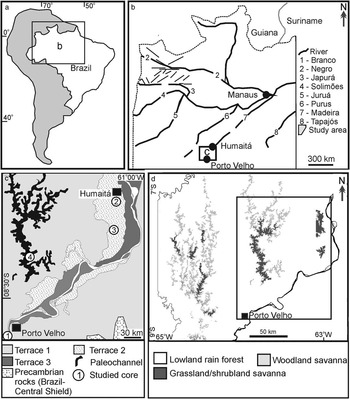
Figure 1 (a,b) Location of the study area between Porto Velho and Humaitá, southwestern Amazonia, Brazil (a), with indication of main river systems and tectonic lineaments (b). (c) Study area with location of fluvial terraces and the four studied cores (modified from Rossetti et al. Reference Rossetti, Cohen, Bertani, Hayakawa, Paz, Castro and Friaes2014). (d) Main vegetation types in the study area. Inner box indicates the study area shown in Figure 1c.
PHYSIOGRAPHY AND GEOLOGICAL FRAMEWORK
The study area is located between the city of Porto Velho in the north of the State of Rondonia and the town of Humaitá in the south of the State of Amazonas (Figure 1a,b). Climate in this region is characterized by short dry seasons (Am in Köppen’s classification) and a mean annual temperature of 28°C, with a minimum of 10°C in June and July. Precipitation averages 2500 to 3000 mm/yr and the relative humidity is 85%. Vegetation is chiefly arboreal, including lowland Ombrophyla forest in sharp contact with large patches of open vegetation, mostly grassland and shrubland (Figure 1d) (Radambrasil Reference Radambrasil1978).
Geologically, the study area is within the Solimões Basin, which is a 600,000-km² intracratonic Paleozoic rift that evolved into a foreland basin in the Cretaceous and Cenozoic due to intraplate extension and tectonic uplifts in the Andean Chain. Cenozoic deposits in this basin consist of the Solimões and Içá Formations (Cunha et al. Reference Cunha, Gonzaga, Coutinho and Feijó1994), as well as unnamed Pleistocene−Holocene deposits (Rossetti et al. Reference Rossetti, Toledo and Góes2005). In the study area, the latter deposits consist of three tectonically influenced fluvial terraces formed before 43,500 and 31,696–32,913 cal yr BP (terrace T1), between 25,338–26,056 and 14,129–14,967 cal yr BP (terrace T2), and between 12,881–13,245 to 3158–3367 cal yr BP (terrace T3) (Rossetti et al. Reference Rossetti, Cohen, Bertani, Hayakawa, Paz, Castro and Friaes2014; Figure 1c).
MATERIALS AND METHODS
This study was based on four continuous cores of up to 10 m long each (Figure 1c), acquired with a percussion drilling Robotic Key System (RKS), model COBRA mk1 (COBRA Directional Drilling Ltd., Darlington, UK). Cores 2 and 4 are novel, while cores 1 and 3 correspond respectively to the cores designated as HU-1 and PV02 in a previous publication (Cohen et al. Reference Cohen, Rossetti, Pessenda, Friaes and Oliveira2014). The two latter cores were included in the present work because these authors focused only on pollen data, having provided no detailed analysis of isotope data or facies interpretation. Facies analysis was based on measured lithostratigraphic profiles containing information such as lithology, texture, sedimentary structure, and type of contact. The description of various fluvial paleomorphologies was based on the analysis of remote sensing data including Landsat 5−TM images (www.dgi.inpe.br) and a digital elevation model (DEM) from the Shuttle Radar Topography Mission (SRTM) (ftp://e0srp01u.ecs.nasa.gov/srtm/). The optical images were registered and processed for R (red), B (blue), G (green) band composition. The SRTM−DEM consisted on the C-band original 90-m resolution (3 arc seconds) obtained with synthetic aperture radar. The SRTM data were processed using customized shading schemes and palettes in the Global Mapper Software 2009 in order to highlight the features of interest. High-resolution QuickBird and SPOT optical images from Google Earth helped in analyzing the paleomorphologies in more detail and establishing their relationship to vegetation cover.
For the total organic carbon (TOC), total nitrogen (TN), and isotope analyses, 76 core samples were systematically collected at 20-cm intervals along the studied cores. Homogenized bulk samples were oven-dried at 50°C for 48 hr. A parcel (~1 g) of each sample was acidified with 1.5M HCl and left overnight to allow inorganic carbon to be liberated as CO2. The samples were then repeatedly washed with distilled water to remove inorganic carbon and subsequently oven-dried at 60°C. The analyses were performed at the Nuclear Energy Center of Stable Isotopes and Agriculture Laboratory (CENA/USP). TOC and TN measurements were carried out on an elementary analyzer attached to a Mass Spectrometry ANCA SL 2020 of Scientific Europa. The results are expressed in % of dry weight for the total C and N. The isotopes ratios are provided in ‰ with respect to the VPDB (Viena Pee Dee Belemnite) standard for the δ13C and atmospheric air for the δ15N, both with analytical precision greater than 0.2‰. Replicates were produced for every five samples analyzed. The C/N values represent the molar ratio between TOC and TN, calculated based on the following equation: C/Nmolar=(%TOC/12.011)/(%TN/14.007).
The chronological control was obtained from 22 samples of bulk sediments. Sampling did not follow a regular spacing, but it depended on the availability of fresh muddy sediments rich in organic carbon. The samples were collected aiming to record a succession of age variation with depth to each profile. Sample pretreatment and dating followed the Beta Analytic Radiocarbon Dating Laboratory (Miami, USA, lab code Beta-) standard technique for AMS dating. The pretreatment consisted of dispersing the sediment deionized water, followed by sieving through a 180-micron sieve to recover any available plant material and to remove any stones, gravels, or other course inorganic grains. The <180-micron size fraction was used in each case. Two 0.1N HCl baths were applied for 2 hr each at 70°C to remove any carbonates. Samples were rinsed to neutral and dried at 100°C for 12 hr, cooled, and weighed. After homogenizing with a mortar and pestle, a small portion of the sediment was tested under a microscope with 12M HCl to ensure complete removal of all carbonate. Each sample was subsampled and combusted to CO2 in a closed chemistry line, which had been purged of any CO2 to a level below 10e–15 atoms (background levels). The CO2 was then introduced into a reaction vessel containing an aliquot of cobalt metal catalyst. Hydrogen was introduced such that when the cocktail was heated to 500°C, the CO2 cracked to carbon (graphite). The graphite was pressed into a target for measurement in the AMS. The AMS was calibrated to provide an accurate ratio of the 14C/13C ratio between the sample graphite and a modern reference (NIST-4990C, oxalic acid). Quality assurance (QA) samples were reacted simultaneously in the chemistry lab and measured simultaneously in the AMS. The analytical result was obtained as a fraction of the modern reference, corrected for isotopic fractionation using 13C/12C (δ13C) and the 14C age was calculated according to the convention of Stuiver and Polach (Reference Stuiver and Polach1977). The QA samples were checked for accuracy and observed to fall within expectations for the laboratory to accept and report the sample results. The QA acceptance was defined as the total laboratory error known to be within 2σ. The equipment used in these analyses was the Thermo Delta-Plus isotope ratio mass spectrometer (δ13C precision of ±0.3‰) and a 250kV NEC single-stage particle accelerator (AMS precision of ±0.001–0.004 fraction modern). 14C ages are reported in years before AD 1950 (yr BP) normalized to a δ13C of –25‰VPDB and in cal yr BP according to SHCal13 (Reimer et al. Reference Reimer, Bard, Bayliss, Beck, Blackwell, Ramsey, Buck, Cheng, Edwards, Friedrich, Grootes, Guilderson, Haflidason, Hajdas, Hatté, Heaton, Hoffmann, Hogg, Hughen, Kaiser, Kromer, Manning, Reimer, Richards, Scott, Southon, Staff, Turney and van der Plicht2013). The software CALIB v 7.1 html was used for age calibration.
RESULTS
Morphological Context and Sedimentology
The studied cores were acquired along fluvial terraces at the margin of the Madeira River (Figure 1c). These terraces have altitudes ranging from 100–85 m (oldest), 85−65 m, and 65−45 m (youngest), the latter located closer to the modern river valley. Core 1 stands at an altitude of 57 m, being inserted in the lowermost fluvial terrace (T3) less than 300 m from the margin of the modern Madeira River (Figure 2a). Vegetation in this site consists of seasonally flooded Ombrophyla forest. Core 2 occurs at an altitude of 67 m over the second fluvial terrace (T2) (Figure 2b–d). The southern part of this terrace contains a large paleomeander belt nearly 2.5 km wide (Figure 2b,c), which is covered in part by grassland and in part by Ombrophyla dense alluvial forest (Figure 2c,d). Core 2 was plotted in a grassy floodplain located northeastward of the paleomeander (Figure 2d). Core 3 (Figure 2b,e) is also located in an area of open vegetation corresponding to a paleomeander of terrace T2. Core 4 is located at 79 m altitude in an area of open vegetation corresponding to a paleochannel in the uppermost (oldest) terrace (i.e. T1) of the Madeira River (Figure 2f,g).

Figure 2 Geomorphological context of the studied cores. (a) Core 1 located in a primarily seasonally flooded area (now anthropogenically-modified nonforested area) located in the lowest fluvial terrace of the Madeira River (QuickBird image, Image 2007–Digital Globe). (b) DEM–SRTM locating two large savanna patches over an intermediate terrace of the Madeira River, where cores 2 and 3 were plotted. Note that the first core occurs in a large savanna area corresponding to a floodplain paleoenvironment, and the second one in a savanna area developed over a paleomeander. (c,d) Landsat (c) and QuickBird image (Image 2007–Digital Globe) (d) with detailed view of the paleomorphology and floristic composition in the areas corresponding to cores 2 and 3. Note in (c) the semi-circular shape with several concentric lines corresponding to a paleomeander in sharp contact (hatched line) with its associated paleofloodplain. Note also the sharp contrasts between savanna (pink) and forest (green) (colors correspond to the online color version of the article); (e) Detail of the site of core 3, acquired also over a paleomeander displaying several concentric lines representative of channel migration through time (QuickBird image, Image 2007–Digital Globe). (f) DEM–SRTM illustrating the place where core 4 was acquired. Note that this core was plotted over a large, elongated belt of savanna, which highlights a southward trending paleodrainage system. (g) Detailed view of site 4, illustrating the floristic types (QuickBird image, Image 2007-Digital Globe).
The cores consist of sandy and muddy lithologies, with cores 1 and 2 being the muddiest ones and core 4 the sandiest one. Three facies associations are present, hereafter designated as FAA, FAB, and FAC, which correspond respectively to the following paleoenvironments: active channel, abandoned channel, and floodplain complex (Figures 3–6).

Figure 3 Litostratigraphic profile of core 1, with the vertical distribution of sedimentary facies, depositional environments, ages, δ13C, δ15N, and C/N. Note that ages are cal (ka) BP.

Figure 4 Litostratigraphic profile of core 2, with the vertical distribution of sedimentary facies, depositional environments, ages, δ13C, δ15N, and C/N. Note that ages are cal (ka) BP.

Figure 5 Litostratigraphic profile of core 3, with the vertical distribution of sedimentary facies, depositional environments, ages, δ13C, δ15N, and C/N. Note that ages are cal (ka) BP.

Figure 6 Litostratigraphic profile of core 4, with the vertical distribution of sedimentary facies, depositional environments, ages, δ13C, δ15N, and C/N. Note that ages are cal (ka) BP.
FAA is up to 4 m thick, occurs only in cores 3 and 4, and is characterized by sharp erosional bases mantled by cross-stratified sandstone that grade upward into massive sandstone. The base of FAA in core 3 was not reached. The lithologies form fining-upward successions varying upward from medium/coarse-grained sandstone to very fine-grained sandstone, which are moderately to well sorted and mostly composed of quartz grains.
FAB, also restricted to cores 3 and 4, grades upward from FAA and is up to 3 m long in core 4 and only 0.6 m in core 3. Deposits in FAB consist of three lithofacies: very fine- to fine-grained massive sandstone, parallel-laminated mudstone, and heterolithic deposits. The latter includes mudstone with lenses of silty or very fine- to medium-grained sandstone internally massive or trough cross-laminated; undulating silty and very fine- to medium-grained sandstone interbedded either with laminated or massive mudstone; and mudstone lenses within fine- to medium-grained sandstone. These lithofacies configure fining-upward successions.
FAC is recorded in all cores, being more expressive in cores 1 and 2. This association occurs on top of FAB in cores 3 and 4, completing its overall fining-upward nature. The lithologies consist of parallel-laminated mudstone that grades upward into indurated massive mudstone and pelite with roots and/or root marks. Organic plant debris are present and iron oxides/hydroxide nodules (a few mm in diameter) are dispersed in these deposits. Thin (i.e. up to 0.3 m thick) beds of massive silty to very fine-grained sandstone are also present and they grade downward from parallel-laminated mudstone and lenticular heterolithic deposits forming coarsening-upward successions. Alternatively, sandy layers are interbedded with laminated mudstone as rhythmites.
Radiocarbon Chronology
14C analyses of the studied deposits (Table 1) revealed Late Pleistocene and Holocene ages ranging from 42.8–41.8 to 2.3–2.2 cal ka BP. The lower half of core 3 recorded the oldest ages (i.e. 42.8–41.8 to 35.0–34.3 cal ka BP). Upward, these deposits displayed a paleosol horizon that indicates a hiatus, which was confirmed by the contrasting ages (i.e. 16.9–16.3 and 7.3–7.2 cal ka BP) of the overlying deposits. The second oldest age succession was recorded at 8.4–2.6 m of core 2, which varied upward from 26.0–25.5 cal ka BP to 22.1–21.4 cal ka BP. Similarly to core 3, this core also recorded a hiatus, with deposits above 2.6 m having ages of 5.5–5.3 and 4.4–4.2 cal ka BP. As expected by the location in the lowest terrace, the youngest age set was found in core 1, which varied from 11.1–10.7 to 3.4–3.1 cal ka BP in the last 4 m. Below this depth, three other ages were recorded from bottom to top, i.e. 10.8–10.6, 7.3–7.0, and 9.7–9.5 cal ka BP. This age succession recorded a time inversion. The presence of a palosol at these depths led to suggest that this may have occurred due to carbon rejuvenation by contamination with new carbon available when the sediments where subaereally exposed to pedogenesis (Figure 4). Core 4 showed continuous mud with ages ranging upward from 22.4–22.0 to 2.3–2.2 cal ka BP. However, a younger age of 7.2–7.0 cal ka BP was recorded at 8.3–8.2 m depth, which was also related to contamination by new carbon during pedogenesis.
Table 1 Radiocarbon ages of the studied deposits.

Considering the provided calibrated ages, the sedimentation rates of the studied cores varied from about 0.2 (cores 3 and 4) to 0.3 (core 2) or up to 0.7 (core 1) mm yr–1. These rates are presented only as a broad view on sedimentation rates, as these were calculated assuming that sedimentation remained constant through time, which may not be true in all instances.
Isotopic and Chemical Data
δ13C, δ15N, and C/N data varied largely, i.e. δ13C=–30.1 to –14.6‰, δ15N=1.3 to 9.2‰, and C/N=0.6 to 16.7 (Figures 3−6). The TOC and TN values were generally low in all cores, being <1.6% and 0.2%, respectively. These proxies displayed similar patterns of variation within and among individual profiles. Most of samples in core 1 (Figure 3) had δ13C values of –28.9 to –22.9‰ and C/N values of 2.4 to 10.0. At 6.8 m depth, the C/N was as high as 10.0, the δ13C was the most depleted (i.e. –30.1‰), while the δ15N was as low as 1.3‰. Between 6.6 m and 4.2 m, the C/N (2.4 to 5.1) and δ15N (2.6 to 3.7‰) increased, while δ13C progressively enriched from –29.4 to –27.2‰. Above this depth, the δ13C oscillated between –27.5 and –25.9‰, the C/N oscillated between 3.3 and 2.1, and then suddenly increased to 4.1 to 6.5 between 0.6 and 0.2 m depth, and the δ15N progressively increased from 3.1 to 6.4‰.
Up to 4.2 m depth in core 2 (Figure 4), the δ13C oscillated from –27.6 to –22.9‰, the C/N from 0.7 to 2.0, and the δ15N from 3.2 to 7.2‰. An exception occurs between 8.0 and 7.2 m depth, where δ13C was as depleted as –22.9‰, C/N was as high as 7.5, and δ15N was as low as 2.6‰. Above 4.2 m depth, there was a progressive enrichment in δ13C, with sudden peak of –15.9‰ at 0.4 m depth, which was accompanied by an increase in C/N to 11.3 and a decrease in δ15N to 2.5‰. Upward and after some oscillation, there was another remarkable peak of δ13C enrichment to 18.6‰, while the C/N was as high as 37.6 and the δ15N decreased from 5.0 to 3.3‰.
Core 3 (Figure 5) displayed the highest recorded range for all values, with δ13C=–28.1 to –14.9‰, δ15N=1.8 to 9.2‰, and C/N=0.9 to 16.7. The most striking finding is that, after several oscillations into depleted values, the δ13C values were enriched to –14.59‰ at 2 m depth and upward. Below around 5.4 m depth, the δ13C and C/N were highly oscillating, varying from –28.2 to –20.2‰ and 4.6 to 16.7, respectively. After several oscillations, the C/N had the lowest value (i.e. 2.0) at 3.8 m, increasing upward to 12.2. The marked change of δ13C values from –20.9 to –16.9‰ at around 1.2 m depth is interesting, with this proxy remaining enriched upward. This enrichment in δ13C coincides with increased C/N, which had peaks at 1 m depth of 11.5 and above 0.2 m depth of 12.2 to 12.1. Meanwhile, δ15N progressively increased to a peak of 9.2‰, decreasing at the top to 6.2‰.
Values of δ13C, δ15N, and C/N along core 4 (Figure 6) were distributed more uniformly than in the previous cores, with a sudden change at 1.2 m depth. Hence, below 1.2 m, δ13C was –28.0 to –24.2‰, with one value of –29.1‰ at 7 m, δ15N is 1.6 to 7.0‰, and C/N is 0.6 to 2.7, with one value of 4.4 at 1.6 m. Above 1.2 m, the δ13C values were enriched up to –15.56‰, while the δ15N is 4.8–7.9‰, and the C/N is 4.3–9.2. At 0.6 m depth, the δ13C varied from –23.5 to –19.6‰ and then –12.7‰ and the C/N varied from 4.4 to 9.1 and then 9.2, while δ15N varied from 5.4 to 7.9‰.
DISCUSSION
Paleoenvironmental Evolution and Plant Contribution through Time
Our faciological and chronological data indicate that the studied cores contain sedimentary deposits typically accumulated in fluviatile environments during the last 43 ka BP. The δ13C, δ15N, and C/N values of these deposits allowed to infer changes in vegetation over this time interval. A prior consideration before using these proxies for this purpose is that these signals detected in the sedimentary record may differ from contemporaneous plants mostly due to one or a combination of the following factors: (i) biodegradation by aerobic microbes during and after sediment deposition (Thornton and McManus Reference Thornton and McManus1994; Cloern et al. Reference Cloern, Canuel and Harris2002; see also references in Lamb et al. Reference Lamb, Wilson and Leng2006 and Chen et al. Reference Chen, Zhang, Yang and Zhang2008); (ii) biosynthesis of inorganic nitrogen (Meyers Reference Meyers1997; Chen et al. Reference Chen, Zhang, Yang and Zhang2008); (iii) incorporation of different amounts of organic matter by various grain sizes (e.g. Keil et al. Reference Keil, Tsamakis, Fuh, Giddings and Hedges1994); (iv) postdepositional chemical or biogenic modifications (see Chen et al. Reference Chen, Zhang, Yang and Zhang2008 for a review); and (v) increased atmospheric CO2 by ~20% since the LGM, which may affect the δ13C values (Adams et al. Reference Adams, Faure, Faure-Denard, McGlade and Woodward1990). Despite these potential interferences, a primary nature of the δ13C and C/N values recorded in the study area is suggested by their non-random vertical distribution and good correspondence when deposits of similar ages are compared; many variations within a same facies association, indicating they are facies-independent; and the good agreement between plant types interpreted from these data and published pollen data from same profiles (see Cohen et al. Reference Cohen, Rossetti, Pessenda, Friaes and Oliveira2014), as discussed below.
Previous works based only on δ13C values of sedimentary deposits from the study area related changes from C3 to C4 land plants to directly alternating wet and dry phases (Pessenda et al. Reference Pessenda, Gomes, Aravena, Ribeiro, Boulet and Gouveia1998, Reference Pessenda, Boulet, Aravena, Rosolen, Gouveia, Ribeiro and Lamotte2001, Reference Pessenda, Ribeiro, Gouveia, Aravena, Boulet and Bendassoli2004, Reference Pessenda, Ledru, Gouveia, Aravena, Ribeiro, Bendassolli and Boulet2005). However, a comparison of data from the studied deposits with those from modern vegetation allowed detecting changes in vegetation types through time and also analyzing their potential causes considering the paleoenvironmental framework provided by facies analysis. For the discussion below, sedimentation rates were used to estimate ages in stratigraphic intervals lacking these data.
Our results indicated generally low C/N values (i.e. usually <12), which are more compatible with the prevalence of freshwater phytoplankton than land plants, the latter occurring only at certain stratigraphic intervals displaying C/N>12. Both C3 and C4 land plants were present, with the first being recognized by δ13C values comparable to those from a number of Amazonian trees, i.e. –37.8 to –25.9‰ (Ometto et al. Reference Ometto, Ehleringer, Domingues, Berry, Ishida, Mazzi, Higucji, Flanagan, Nardoto and Martinelli2006) or –37.8 to –28.9‰ (Francisquini et al. Reference Francisquin, Lima, Pessenda, Rossetti, França and Cohen2014) and also from modern soils of this region, i.e. usually <–27‰ (Magnusson et al. Reference Magnusson, Sanaiotti, Lima, Martinelli, Victoria, Araújo and Albernaz2002).
The base of core 3, which corresponds to an uncertain age that approaches the limit of the 14C dating technique, recorded the establishment of a fluvial channel. Although the basal channel surface was not reached in this core, this interpretation is provided by the upward gradation from FAA into FAB and FAC configuring a fining-upward succession, which matches with descriptions of many channel deposits (e.g. Atchley et al. Reference Atchley, Nordt and Dworkin2004; McLaurin and Steel Reference McLaurin and Steel2007). Sand was formed at the bottom of this channel for a certain period of time. However, before 42.8–41.8 cal ka BP, it declined in energy, with alternating sand and mud deposition continuing up to 39.0–38.0 cal ka BP. A varied contribution of different types of organic matter was expected during the active and gradual phase of channel abandonment. This is due to the possibility of having various environments with diverse plant types cut by the channel along its drainage basin. Indeed, the high fluctuation of δ13C from –28.2 to –20.2‰ and C/N from 4.6 to 16.7 recorded in the channel deposits at around 5.4 m depth in core 3 suggests a mixture of phytoplankton with C3 and C4 land plants (Figures 5 and 7). Despite frequent oscillations, the progressive increase in C/N values, accompanied by the enrichment in δ13C, are consistent with the increased contribution of C4 land plants through time. The upward change from fluctuating and higher δ15N values into more uniform and lower values is in agreement with the presence of land plants.

Figure 7 Types of organic matter preserved in the sedimentary deposits of the study area, contrasted to the history of global ice fluctuation since near the last glacial episode (i.e. ~60 ka ago) [see text for discussion; curve of global ice after Crowley and North (Reference Crowley and North1991); δ18O stages from Emiliani (Reference Emiliani1955) and Shackleton (Reference Shackleton1969); ages are in cal yr BP; figure modified from Rossetti et al. (Reference Rossetti, Cohen, Bertani, Hayakawa, Paz, Castro and Friaes2014)].
Core 3 recorded also the time interval before 39.0–38.0 to 35.0–34.3 cal ka BP, when following a period of slowly declining energy, the channel became completely abandoned, as indicated by only mud settling from suspensions in low-energy environments (i.e. facies association FAC). Such an environmental context favors sediments with in situ organic matter. Thus, the sudden depletion in δ13C and decrease in C/N during this time are consistent with the prevalence of freshwater phytoplankton in this initial phase of channel abandonment.
Considering the estimated sedimentation rate of 0.2 mm yr–1, the two time ranges discussed above were also represented in the lower part of core 4. As in core 3, a channel interpretation for these temporally corresponding deposits was confirmed by the upward transition from facies associations FAA, FAB to FAC, indicative of decreasing flow energy with time. The sharp erosional base of FAA is compatible with a confined environment, typical of channels. Bedload transport within the active channel is recorded by the sandy deposits overlying the basal surface, and the cross-stratification indicates bedform migration at the channel bottom under low flow regime. Thus, sand started filling up a channel environment in core 4 just before ~40.0 cal ka BP, when the channel recorded at core 3 was already abandoned. Despite these differences in sedimentary facies, the isotope and C/N signals of these two sedimentary channel successions are comparable, confirming the increment of organic matter derived from phytoplankton after ~40.0 cal ka BP.
The interval between 26.0–25.5 and 22.1–21.6 cal ka BP is well represented in core 2, where the sedimentary record indicated the prevalence of mud deposition from suspensions in a low energy environment. The large volume of parallel-laminated mudstone formed during this time interval at this locality attests mud settling from suspensions, while the thin sandstone layers were due to episodes of relatively higher energy flows. The two coarsening-upward successions between 3 and 4 m in core 2 (Figure 4), suggestive of eventual flooding with development of crevasse splays, and the location of this core marginally to a paleomeander (core 2), support deposition in a floodplain and/or oxbow lake environments. While these floodplains were developing, the channel at core 4 became abandoned. This history is also represented in core 3, although a period of erosion and soil development (see 3.8 m depth in Figure 6) may have destroyed part of the sedimentary record at this locality. Independently of the dissimilar sedimentary history, these cores displayed analogous δ13C and C/N trends that either remained with persistently depleted δ13C and extremely low C/N values, or showed an upward trend into slight enrichment of δ13C and higher C/N values. An exception is the lower part of core 2 between 8.0 and 7.2 m depth, where δ13C was as depleted as –22.9‰, which may be related to an episodic higher contribution of land plants. It is interesting to note that the δ13C values in this depth interval were more enriched than those recorded in leaves from the modern forest, which supports a slow increment in C4 plants. It follows that the early phase of the LGM in southeastern Amazonia may have had flooded fluvial environments with organic matter derived mainly from phytoplankton, but with episodic contribution of probably C4 land plants. The fact that the δ15N values are mostly from 4.0 to nearly 8.0‰ is in agreement with aquatic plants, at the same time that its decrease to values as low as 2.6‰ between 8.0 and 7.2 m depth coincides with the suggested episodic contribution of C4 land plants.
After ~22.0 cal ka BP, muddy deposition occurred in all cores. This is represented in core 4 by the complete channel abandonment. This phase is recorded by the upward gradation from FAA to FAB and then FAC, a sedimentary succession including heterolithic and muddy deposits related to decreasing flows. Considering that the channel morphology is still preserved at the surface in this core, and also in core 3, the most likely hypothesis is that the essentially muddy deposits from the uppermost part of these successions (i.e. FAC) record oxbow lakes formed after channel abandonment. The soil profile at 1.4 m depth in core 3 indicates an episode of nondeposition and/or erosion. This event may have been local, as it was not recorded in core 4, which seems to record continuous sedimentation. The muddy deposits formed along core 1 and also after 22.0–21.6 cal ka BP in core 2 are thicker and probably record floodplains, which is suggested by their location in a young terrace close to the modern Madeira River (core 1) and marginally to a paleomeander (core 2).
The upward enrichment of δ13C, accompanied by higher C/N along the oxbow lake and floodplain deposits from the end of the LGM, suggests an increased contribution of C4 land plants, particularly in the Holocene. Interestingly, this trend was recorded only in cores located where the modern landscape is also characterized by grassland and shrubland (i.e. cores 2, 3, and 4). In core 2, this trend was evidenced by an enrichment in δ13C to –15.0‰, while the C/N, although still low, was increased to 11.3 at 5.3–5.5 cal ka BP. Following a short episode of very low C/N suggestive of phytoplankton, the trend to C4 land plants was evidenced upward in this core by the highest C/N values of 37.6, with enriched δ13C of 18.6‰; the δ15N corresponding to this depth displayed a value (3.3‰) commonly related to terrestrial plants. The sudden increased contribution of C4 land plants in core 3 may have occurred earlier, i.e. before 7.3–7.2 cal ka BP at ~1.2 m depth, when δ13C varied from –20.9 to –16.9‰. However, the maximum C4 contribution occurred at 1 m and above 0.2 m depths, when C/N values were higher, i.e. 11.5 and 12.2–12.1, respectively. A contribution of C4 land plants was recorded also in core 4 before 2.3–2.2 cal ka BP (0.6–0.4 m depth), when δ13C varied from –23.5 to –19.6 and then –12.7‰. The corresponding C/N variations from 4.4 to 9.1 and then 9.2 at these depths perhaps indicate the mixing of C4 land plants with phytoplankton; the abrupt decrease in δ15N is in agreement with these changes. The sudden C/N increase and δ13C enrichment around the mid-Holocene may reflect C4 grasses sourced either from land areas around the drainage basin or locally unflooded areas. Although C3 grasses occur in the humid Amazonian lowland (e.g. Lima Reference Lima2008), grasses from modern floodplains do have δ13C values compatible with C4 land plants (i.e. –12.0 to –15.0‰; cf. Victoria et al. Reference Victoria, Martinelli, Trivelin, Matsui, Forsberg, Richey and Devol1992).
Different from the other cores, core 1 is located in an area with modern forest. This core, which has the highest sedimentation rate (i.e. up to 0.7 mm yr–1), is interesting because it records the entire Holocene. An episode of increased concentration in C3 vascular plants at an uncertain age before the Holocene is possibly represented by δ13C as depleted as –30.1‰ at ~6.8 m depth (Figure 3); this suggested land plant influence is in agreement with the low δ15N values of 1.3‰. However, the corresponding C/N was still low (i.e. up to 10.0), attesting phytoplankton, probably with some contribution of C3 land plants (Figure 3) until ~11.1–10.7 cal ka BP, when the change into even lower C/N values suggests the increased contribution of phytoplankton. Only at ~3.4–3.1 cal ka BP the C/N slightly increased, probably due to the progressive contribution of C3 land plants during the establishment of the overlying forested landscape. The soil profile dated at 6.5–6.3 cal ka BP recorded a local hiatus not recorded in any of the other cores.
Controls on Plant Distribution through Time: Climate Versus Sedimentary Dynamics
Despite the incomplete temporal record of individual sites, the studied cores represent an almost continuous testimony of sedimentation in southwestern Amazonia for most of the LG and also the Holocene. Thus, they provide significant data for reconstructing vegetation changes and analyzing the climate variations during this time.
Previous publications have considered two scenarios for explaining vegetation changes during the late Quaternary in Amazonia. The first scenario considers alternations from wet (warm) to dry (cold) periods mainly based on the presence/absence of forest and herb pollen (e.g. van der Hammen and Absy Reference van der Hammen and Absy1994; Behling and Hooghiemstra Reference Behling and Hooghiemstra1999; Behling and Costa Reference Behling and Costa2000, Reference Behling and Costa2001; Mayle et al. Reference Mayle, Burbridge and Killeen2000; Haffer Reference Haffer2001; Sifeddine et al. Reference Sifeddine, Marint, Turcq, Volkmer–Ribeiro, Soubiès, Cordeiro and Suguio2001; van der Hammen Reference van der Hammen2001). The second paleoclimatic scenario depicts a relatively undisturbed Amazonian rainforest during the last 50,000 yr (e.g. Colinvaux et al. Reference Colinvaux, Oliveira, Moreno, Miller and Bush1996, Reference Colinvaux, Oliveira and Bush2000, 2001; Bush et al. Reference Bush, Oliveira, Colinvaux, Miller and Moreno2004; Irion et al. Reference Irion, Bush, Mello, Stüben, Neumann, Müller, Moraes and Junk2006; Mayle and Power Reference Mayle and Power2008; Toledo and Bush Reference Toledo and Bush2008). Most of the available palynological data (Figure 7) indicate three episodes of savanna expansion in eastern Amazonia for the Late Pleistocene (i.e. >51.0 14C ka BP, 40.0 14C ka BP, and 23.0−11.0 14C ka BP) (Absy et al. Reference Absy, Cleef, Fournier, Martin, Servant, Sifeddine, Silva, Soubié, Suguio, Turcq and van der Hammen1991). The climate was wet in the Late Pleistocene before the LGM in Carajás (Absy et al. Reference Absy, Cleef, Fournier, Martin, Servant, Sifeddine, Silva, Soubié, Suguio, Turcq and van der Hammen1991), although a dry period was recorded in Laguna Bella Vista (Mayle et al. Reference Mayle, Burbridge and Killeen2000). Although without a direct effect on the forest, Lake Pata also had the lowest lake level between 35−23 14C ka BP (Colinvaux et al. Reference Colinvaux, Oliveira and Bush2000). Forest was recorded in the Katira area in the State of Rondonia before 49.0 14C ka BP, with its replacement by savanna between 41.0 and 18.0 14C ka BP (van der Hammen and Absy Reference van der Hammen and Absy1994). In addition, paleontological (Webb and Rancy Reference Webb and Rancy1996; Vivo and Carmignotto Reference Vivo and Carmignotto2004; Rossetti et al. Reference Rossetti, Toledo, Moraes–Santos and Santos2004) and geological (Bibus Reference Bibus1983; Sifeddine et al. Reference Sifeddine, Marint, Turcq, Volkmer–Ribeiro, Soubiès, Cordeiro and Suguio2001) data suggest a Late Pleistocene climate drier than in the present.
The detailed analysis of isotope and C/N data and their distribution along the studied cores showed no clear record of plant types that could be related exclusively to arid climate before 39.0–38.0 cal ka BP. This timeframe is particularly well represented in cores 3 and 4, which were related to paleomeanders of the Madeira River. This river has a regional expression, being one of the most extensive Amazonian tributaries and the fifth longest river in the world. Thus, the organic matter content present in cores 3 and 4 may have reflected the overall floristic composition over a wide range of environments in the region, being useful for discussing the climate prevailing over this drainage basin. The prevalence of phytoplankton in cores 3 and 4 before 39.0 to 38.0 cal ka BP (Figure 7) may suggest a dominance of wet conditions with widespread flooded areas. The subordinate occurrence of C4 land plants in these cores could signify that the overall wet period alternated with short dry episodes. This climatic interpretation for the study area is in good agreement with the prevalence of wet climate with short dry periods in the Katira site (van der Hammen and Absy Reference van der Hammen and Absy1994). It is also concordant with the alternation of forest and savanna proposed for the Carajás site (Absy et al. Reference Absy, Cleef, Fournier, Martin, Servant, Sifeddine, Silva, Soubié, Suguio, Turcq and van der Hammen1991) during this time interval. Interestingly, the clearest increase of C4 land plants recorded around ~40.0 ka BP in the study area matches well with a dry phase in the Katira and Carajás sites, as well as in the Laguna Bella Vista (Mayle et al. Reference Mayle, Burbridge and Killeen2000).
The climatic record between ~40 ka BP and the onset of the LGM in Amazonia is more variable, with sites such as Carajás, and probably also Katira, indicating wet conditions with forest expansion, while other areas, such as Lake Pata, recorded the lowest lake level related to a maximum dry phase, although without a clear effect in the rainforest (Colinvaux et al. Reference Colinvaux, Oliveira and Bush2000; Figure 7). In addition, following a dry phase just after 40.0 cal ka BP, Laguna Bella Vista also had a wet and warm climate, which would have favored the rainforest expansion (Mayle et al. Reference Mayle, Burbridge and Killeen2000). Our data show deposits with a prevalence of phytoplankton after 38.0 cal ka BP, a trend that continued through the LGM. In addition, previously published pollen data from two of our studied cores (i.e. cores 1 and 2) point to wet, but cold-adapted, plants in association with herbs and tree taxa similar to modern ones at least between 42.6 and 35.2 cal ka BP (Cohen et al. Reference Cohen, Rossetti, Pessenda, Friaes and Oliveira2014). These data are interesting because they suggest the continuing cold but humid conditions in this Amazonian region toward the onset of the LGM. When these cold-adapted plant species disappeared from the study area remains to be determined, but they did not last until the Holocene (Cohen et al. Reference Cohen, Rossetti, Pessenda, Friaes and Oliveira2014).
Another point of interest derived from our data is the lack of evidence indicating significant vegetation change from the time spanning the LGM. This could suggest the prevalence of aquatic plants as a reflex of a humid climate. While this interpretation is in agreement with the continuous wet climate proposed in Lake Pata (Colinvaux et al. Reference Colinvaux, Oliveira and Bush2000; Figure 7), it conflicts with the dry climate generally proposed for the Amazonian lowlands during this time. For instance, savanna expansion related to a dry climatic phase is recorded in the Carajás site between 23.0 and 11.0 ka BP (Absy et al. Reference Absy, Cleef, Fournier, Martin, Servant, Sifeddine, Silva, Soubié, Suguio, Turcq and van der Hammen1991) and in the Katira site between ~13.0 and 18.0 ka BP (van der Hammen and Absy Reference van der Hammen and Absy1994). In addition, the occurrence of a megafauna in central Amazonian was related to a dry climate at least between 15 and 11.3 ka BP (Rossetti et al. Reference Rossetti, Toledo, Moraes–Santos and Santos2004). Taking these works into account, and also considering the increased contribution of C4 land plants recorded in cores 1, 2, and 3 toward the end of the Late Pleistocene, we argue that the climate may have continued to be cold and humid through the LGM, but probably with episodic droughts towards the end of the period.
The intensified aridity reported until the end of the Late Pleistocene may have crossed the Late Pleistocene–Holocene boundary. However, although the contribution of C4 land plants continued in the Holocene deposits of the study area, there is no evidence to sustain that the sudden increase in this plant type, reported in the uppermost parts of cores 2 to 4, resulted from intensified aridity. A line of evidence leads to suggest that the higher contribution in C4 land plants in these cores is more likely a consequence of sedimentary processes associated with the fluvial dynamics. Firstly, these peaks of C4 land plants were documented only in depositional sites having sediments confined to channel paleolandforms formed in a relatively recent geological time and which are currently covered by herbaceous fields; site 1, which is covered by forest, displayed an almost continuous record of C3 land plants during almost the entire Holocene. It follows that the amplification of herbaceous fields may have occurred only over abandoned channel sites following their infilling, with the resulting sediments being subaereally exposed. Secondly, the modern landscape of cores 2 to 4 contains herbaceous fields despite their location in a tropical humid region, which means that the occurrence of herbs in the mid-Holocene is not necessarily related to dry phases. Thirdly, the peaks with increment of C4 land plants recorded in the cores 2 to 4 were not coeval, being initiated before ~5.5 cal ka BP in core 2, ~7.5 cal ka BP in core 3, and ~2.5 cal ka BP in core 4. Fourth, these ages are also not synchronous with Holocene dry episodes previously proposed for Amazonian areas. For instance, it has been suggested that climate remained dry in this region only until the early to mid-Holocene (Sifeddine et al. Reference Sifeddine, Bertand, Founier, Servant, Soubies, Suguio and Turcq1994; Mayle et al. Reference Mayle, Burbridge and Killeen2000; Mayle and Power Reference Mayle and Power2008) (Figure 7). Other authors also claimed many fluctuations between dry and wet episodes from the early to mid-Holocene (Hughen et al. Reference Hughen, Southon, Lehman and Overpeck2000; Lea et al. Reference Lea, Pak and Spero2000; Pessenda et al. Reference Pessenda, Ribeiro, Gouveia, Aravena, Boulet and Bendassoli2004, Reference Pessenda, Ledru, Gouveia, Aravena, Ribeiro, Bendassolli and Boulet2005), including data from southwestern Amazonia (Pessenda et al. Reference Pessenda, Gomes, Aravena, Ribeiro, Boulet and Gouveia1998, Reference Pessenda, Boulet, Aravena, Rosolen, Gouveia, Ribeiro and Lamotte2001; Freitas et al. Reference Freitas, Pessenda, Aravena, Gouveia, Ribeiro and Boulet2001), but not afterwards. A continuous rainforest was recorded since 7.9 14C ka BP in Caxiuanã (Behling and Costa Reference Behling and Costa2000), 8.3 14C ka BP in Lake Calado (Behling et al. Reference Behling, Keim, Irion, Junk and Mello2001), and 11.0 ka BP in Carajás (Absy et al. Reference Absy, Cleef, Fournier, Martin, Servant, Sifeddine, Silva, Soubié, Suguio, Turcq and van der Hammen1991) (Figure 7). In addition, Lake Pata (Colinvaux et al. Reference Colinvaux, Oliveira and Bush2000) and Lake Katira (van der Hammen and Absy Reference van der Hammen and Absy1994) recorded a wet period throughout the Holocene.
The foregoing discussion leads us to propose an alternative model to explain the peaks of C4 land plants reported in cores 2 to 4. Rather than reflecting dry episodes, our data supports the development of herbaceous fields a few thousand years ago, with their maintenance in the modern landscape being due to the evolution of the fluvial system from river channels into oxbow lakes. As the river cut off took place, a change in the type of organic matter sourced into this depositional system may have occurred. River deposits generally have greater potential to record pollen transported through the drained area, while lake deposits contain organic matter derived from freshwater phytoplankton. Thus, the widespread development of water bodies along floodplains would have resulted in higher phytoplankton production. However, as the lakes were abandoned, the sedimentary deposits exposed to the surface were colonized by herbs. This condition remained up to the present probably due to the maintenance of the water table close to the surface at least during a great part of the year in this wetland.
Therefore, the modern herbaceous fields in the study area could not be linked to past dry climates. The fact that this plant type is confined to paleomorphologies representative of depositional sites that remained active until the Holocene (Figure 2) is consistent with its attribution to sedimentary dynamics as the most likely explanation. This interpretation is also favored because of the overall trend into increased humidity up to 40% after the Young Dryas (Maslin and Burns Reference Maslin and Burns2000), and particularly after the mid-Holocene, when the rainforest spread out over the Amazonian lowland (Sifeddine et al. Reference Sifeddine, Marint, Turcq, Volkmer–Ribeiro, Soubiès, Cordeiro and Suguio2001; Rossetti et al. Reference Rossetti, Toledo and Góes2005).
CONCLUSIONS
This survey integrating δ13C and C/N analyses with sedimentology and 14C chronology was successful for reconstituting changes in vegetation patterns in southwestern Amazonia during the late Quaternary. In addition, despite the limitations due to uncertainties in the fixation mechanisms during nitrogen fractionation pathways, the δ15N values were also generally fairly consistent with C/N variations; thus, they helped the differentiation between organic matter derived from aquatic and land plants. We concluded that the climate was wet with short dry episodes before ~40 cal ka BP. From this time up to the onset of the LGM, humid and cold climate prevailed, with intensified aridity toward the end of the Late Pleistocene. Although this trend continued into the Holocene, the peaks of increased C4 land plant contribution recorded at 5.5 cal ka BP in core 2, ~7.5 cal ka BP in core 3, and ~2.5 cal ka BP in core 4, and the maintenance of herbaceous fields in the modern landscapes of these sites, are related to sedimentary processes due to fluvial dynamics, rather than intensified aridity. Thus, the late Holocene climate was humid, which favored the expansion of the Amazonian rainforest as we see today. The abandonment of channel and lake environments would have favored subaerial exposure and soil development, creating sites favorable for the colonization of herbs of C4 photosynthetic pathway. It follows that great care must be taken when using changes in plant communities for paleoclimatic purpose, as factors other than climate, such as depositional processes, must be also regarded.
Acknowledgments
This work was financially supported by the Brazil’s National Council for Scientific and Technological Development-CNPq (#471483/06-0) and #550331/2010-7 and Research Funding Institute of the State of São Paulo-FAPESP (#13/50475-5). The authors acknowledge the logistic support of the Brazilian Geological Survey-CPRM and the Santo Antonio Hydroelectric during field campaigns. Dr Peter Langdon, as well as two anonymous reviewers, contributed with numerous suggestions and corrections that helped to significantly improve an early version of the manuscript.
SUPPLEMENTARY MATERIAL
To view supplementary material for this article, please visit https://doi.org/10.1017/RDC.2016.107


