2. Experimental set-up and measurements

2.1. Experimental set-up

Although the focus of this paper is on developing a phenomenological model to describe the deformation and orientation dynamics of finite-sized bubbles with any given surrounding flow fields, the experimental data for constraining such a model was not available until recently thanks to the advance of the simultaneous measurements of the bubble 3-D shape and surrounding turbulence. Here, we introduce a unique facility and the associated 3-D simultaneous two-phase measurement technique to aid in developing a phenomenological model for deformable bubbles and drops.

To ensure that the proposed model works for all cases from the buoyancy-dominated to the turbulence-dominated regimes, it is important to develop an experimental set-up that can produce a strong turbulent environment with the turbulence-induced deformation stronger than or at least similar to the buoyancy-induced bubble deformation. This requires that $We\geqslant Eo$ and $We>1$, where the Weber number is defined as $We\approx \rho _c(\langle \epsilon \rangle D)^{2/3}D/\sigma$ based on the Kolmogorov theory. To satisfy this requirement, it is important for $\langle \epsilon \rangle$ to reach approximately $O(0.1)\ \textrm {m}^{2}\ \textrm {s}^{-3}$.

A vertical water tunnel (V-ONSET) was constructed to produce both quiescent and turbulent media. Turbulence in the tunnel was generated by shooting 88 high-speed momentum jets (${\sim }12\ \textrm {m}\ \textrm {s}^{-1}$), through a jet array, into the test section co-axially with the mean flow. All jet nozzles (the nozzle diameter d is 5 mm) were connected to the same high pressure water tank and controlled by a dedicated solenoid valve. The measurement volume of $6\ \textrm {cm}\times 6\ \textrm {cm}\times 5\ \textrm {cm}$ was located about 40$d$ below the jet array. Such a large separation is designed to ensure that the jets are well mixed and that turbulence generated is close to homogeneous and isotropic. A randomized firing pattern of the jets was set similar to that of a previous study by Variano, Bodenschatz & Cowen (Reference Variano, Bodenschatz and Cowen2004), which was shown to generate homogeneous and isotropic turbulence without inducing a persistent mean flow or any secondary flow structures without considering two-way couplings or the bubble–bubble interaction. Detailed discussions of these statistics and flow distributions have been discussed by Masuk et al. (Reference Masuk, Salibindla, Tan and Ni2019b).

In addition to the randomly fired jets, the vertical tunnel features an independently controlled downward mean flow of ${\sim }0.25\ \textrm {m}\ \textrm {s}^{-1}$ to maintain bubbles inside the test section for an extended residence time, which helps to obtain longer bubble trajectories. Bubbles were injected through a capillary island consisting of four arrays of vertically oriented hypodermic needles of two different sizes. After these bubbles reached the interrogation volume, the typical size range of the bubbles turned out to be $D = 2\text {--}7\ \textrm {mm}$. The dimensionless numbers of these bubbles are listed in table 1.

Table 1. Values of the dimensionless parameters used in the model and experiments.

The test section of the tunnel features an octagonal cross-section with eight vertical walls to allow optical access by six high-speed cameras that are uniformly distributed all around the test section. Each of these cameras can operate at 4000 frames per second at a full resolution of 1 megapixel. One dedicated LED panel for each high-speed camera was used to provide diffused back lighting. By using such an optical arrangement, both bubbles and a high concentration of tracer particles (density-matched Polyamide particles with $50\ \mathrm {\mu }\textrm {m}$ in diameter) appeared as dark shadows in front of a bright background. For further description of the tunnel and its diagnostics, the reader may refer to a recent work published by Masuk et al. (Reference Masuk, Salibindla, Tan and Ni2019b).

2.2. Bubble and flow measurements

From raw images, bubbles and tracers were segmented based on their size and contrast difference. Each phase was processed separately to quantify its dynamics. For the fluid phase, an in-house particle tracking code OpenLPT (Tan et al. Reference Tan, Salibindla, Masuk and Ni2020) that utilizes the Shake-The-Box (Schanz, Gesemann & Schröder Reference Schanz, Gesemann and Schröder2016) method was used to obtain the tracer trajectories. For each frame, the centre of each particle was triangulated to obtain its 3-D location, which was then connected through time to acquire the particle trajectory. For the gas phase, a recently developed virtual-camera visual hull method (Masuk, Salibindla & Ni Reference Masuk, Salibindla and Ni2019a) was employed to construct the bubble shape. The 3-D volume of the bubble was first reconstructed by calculating the intersection of the cone-like volume extruding from the bubble shadow on each camera. Then, the shape was refined iteratively by projecting the initial reconstructed volume onto virtual cameras to remove any artefacts generated. In each iteration, the refined geometry was also projected back onto the real cameras to ensure that no real material was removed. Based on the shape reconstruction and refinement, the bubble geometry consisting of many surface vertices can be acquired. These surface vertices can be averaged to determine the bubble centre, which is connected over time, as with how the tracer trajectories were calculated. Both the bubble and tracer trajectories are smoothed by convoluting with Gaussian kernels (Mordant, Crawford & Bodenschatz Reference Mordant, Crawford and Bodenschatz2004), from which the tracer velocity $\boldsymbol {u}^{p}$ and acceleration $\boldsymbol {a}^{p}$ and the bubble velocity $\boldsymbol {u}_b$ and acceleration $\boldsymbol {a}_b$ can be obtained along their trajectories.

Along with each bubble trajectory, two important flow parameters of interest in this study are the fluid velocity at the CoM of a bubble $\boldsymbol {u}_f$ if the bubble is not present and the coarse-grained velocity gradient tensor $\tilde {A}_{ij}$. For every bubble in our experiments, a spherical search volume with diameter $D_s = 2 D$ centred at the bubble CoM was used to select the surrounding tracer particles. Note that for each of these $n$ ($p = 1, 2,\ldots , n$) tracer particles, their velocities and locations have already been determined. The value of $\boldsymbol {u}_f$ is estimated by taking an average of the particle velocity of all $n$ tracer particles, $\boldsymbol {u}_f =\sum _{p=1}^{n} \boldsymbol {u}^{p}/n$. This allows us to calculate the instantaneous slip velocity $\boldsymbol {u}^{s}$ between the two phases: $\boldsymbol {u}^{s}=\boldsymbol {u}_b-\boldsymbol {u}_f$. To obtain the coarse-grained velocity gradient $\tilde {A}_{ij}=\partial u^{p}_i/\partial x^{p}_j$, a least-square fit was performed to minimize the residuals of $\sum _{p}^{} (u^{p}_i - \tilde {A}_{ij}x^{p}_j)^{2}$ using the velocity and location of all $n$ nearby tracer particles. In particular, $\boldsymbol {x}^{p}$ is the separation vector of the $p\textrm {th}$ tracer particle away from the CoM of a bubble. For additional details about the calculation and reliability of such coarse-grained velocity gradients, please refer to previous works by Masuk, Salibindla & Ni (Reference Masuk, Salibindla and Ni2021a) and Ni et al. (Reference Ni, Kramel, Ouellette and Voth2015).

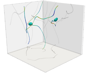
Figure 1 shows examples of the trajectories of deforming bubbles in both (a) quiescent and (b) turbulent media. The trajectories are colour coded with their velocity magnitudes. The zigzag path oscillation is clearly visible in the quiescent rising case, whereas more chaotic trajectories become evident for bubbles travelling in turbulence. In addition to their 3-D trajectories, the shadows they cast on the three main planes are presented to illustrate their projected tracks. Although a high concentration of tracer particles are present, their trajectories are not shown to highlight the difference of bubble tracks in different flows.

Figure 1. Example 3-D bubble trajectories colour coded with their instantaneous velocity magnitude and the 3-D reconstructed shapes at one time instant in (a) an otherwise quiescent medium, and (b) intense turbulence.

2.3. Flow characterization

Before attempting to develop a model for bubble deformation and orientation, the characteristics of the single-phase turbulence generated in our system are briefly discussed here for completeness. Additional details regarding the turbulence characteristics can be found in a recent work by Masuk et al. (Reference Masuk, Salibindla, Tan and Ni2019b). In figure 2, the second-order ($D_{LL}$) and third-order longitudinal structure functions ($D_{LLL}$) are shown, both of which follow the scaling laws for a range of scales that the Kolmogorov theory predicts. Specifically, between $2\eta$ and $200\eta$, $D_{LL}$ appears to exhibit a 2/3 power law, indicated by the dashed line, whereas the power-law exponent seems to be close to 1 for $D_{LLL}$, as indicated by the solid line. Furthermore, the green region in figure 2 indicates the range of the bubble size. It is evident that the bubble size lies within the inertial range, as expected. Moreover, based on the structure function in figure 2, a reasonable estimation of the energy dissipation rate can be obtained, namely $\langle \epsilon \rangle \approx 0.16\pm 0.02\ \textrm {m}^{2}\ \textrm {s}^{-3}$, which satisfies the required turbulence intensity $\langle \epsilon \rangle \approx O$ $(0.1)\ \textrm {m}^{2}\ \textrm {s}^{-3}$ for $We>Eo$. All relevant dimensionless parameters of the generated turbulence can be found in table 1.

Figure 2. The second-order and third-order longitudinal structure functions ($D_{LL}$ and $D_{LLL}$) of turbulence. The green region indicates the range of the bubble size.

3. Finite-sized bubble deformation model (FBD model)

This paper has three main objectives. The first objective is to develop a model to capture the deformation dynamics of finite-sized bubbles with diameter $D$ ($\eta < D< L$) both in turbulence and in water at rest. Second, the developed model should correctly account for two deformation mechanisms driven by the local velocity gradients and the slip velocity between the two phases. For one extreme limit, when bubbles rise in an otherwise quiescent medium, the bubble deformation is dominated by the slip velocity. In this case, $Eo$ is much greater than 1, and $We$ driven by the velocity gradients is close to zero. For the other limit, the turbulent energy dissipation rate becomes so large that the bubble deformation driven by the dynamic pressure gradient ($We\geqslant 1$) becomes important. Finally, the third objective is to use our experimental results to validate the model and constrain different dimensionless coefficients in the model.

Before introducing our model, we begin with the MnM model originally proposed by Maffettone & Minale (Reference Maffettone and Minale1998) to describe the shape evolution of neutrally buoyant droplets in a linear velocity gradient, with the droplet shape represented by a symmetric positive–definite second-order tensor $P_{ij}$, which can be expressed as

(3.1)\begin{equation} \frac{\textrm{d}P_{ij}}{\textrm{d}t}=\varOmega_{ik}P_{kj} - P_{ik}\varOmega_{kj} + f_2(\mu)(S_{ik}P_{kj} + P_{ik}S_{kj}) - \frac{f_1(\mu)}{\tau}(P_{ij} - g(P)\delta_{ij}) , \end{equation}

where the three eigenvalues of $P_{ij}$ represent the squared lengths of three semi-axes of an ellipsoid. Here, $S_{ij}$ and $\varOmega _{ij}$ are the symmetric and anti-symmetric parts of the velocity gradient tensor ($A_{ij}$) that the droplet is subject to. In particular, $S_{ij}=(A_{ij} + A_{ji})/2$ and $\varOmega _{ij}=(A_{ij} - A_{ji})/2$. For a simple shear flow with a small Reynolds number, $f_1$ and $f_2$ are functions of the viscosity ratio $\mu =\mu _d/\mu _c$, where $\mu _d$ and $\mu _c$ represent the dynamic viscosity of the inner fluid of bubbles/drops and their surrounding carrier fluid, respectively. The last term on the right-hand side of (3.1) is the restoring term, in which $\tau =\mu _d D/2\sigma$ is the relaxation time scale of the droplet determined by $\mu _d$ and the coefficient of surface tension $\sigma$; $D$ is the equivalent sphere diameter of the droplet. Volume conservation is ensured in the model with $g(P)=3\text {III}_P/\text {II}_P$, where $\text {III}_P$ and $\text {II}_P$ are the invariants of $P_{ij}$

(3.2a–c)\begin{equation} \text{I}_p=P_{ii},\quad \text{II}_P={-}\tfrac{1}{2}(P_{ij}P_{ij} - \text{I}_P^{2}),\quad \text{III}_P=\tfrac{1}{3}(P_{ik}P_{kj}P_{ji} - \text{I}_P^{3} + 3\text{I}_P\text{II}_P). \end{equation}

This model is suitable for describing the deformation of bubbles in simple flows, and it has been validated against several experimental results (Torza, Cox & Mason Reference Torza, Cox and Mason1972; Bentley & Leal Reference Bentley and Leal1986; Guido & Villone Reference Guido and Villone1998; Guido, Minale & Maffettone Reference Guido, Minale and Maffettone2000). Moreover, the MnM model has been used to characterize the shape evolution of small neutrally buoyant droplets in turbulence (Biferale et al. Reference Biferale, Meneveau and Verzicco2014; Spandan et al. Reference Spandan, Lohse and Verzicco2016). This works under two assumptions: (i) $D$ is in the dissipative range ($D\ll \eta$), where the viscous stress still dominates; and (ii) drops are neutrally buoyant with no significant slip velocity.

For finite-sized bubbles with $D$ in the inertial range ($\eta \ll D\ll L$), neither of these two assumptions holds any longer. In particular, the bubble slip velocity is so large such that the bubble-scale Reynolds number $Re_b$ becomes much larger than one, implying that the flow inertia plays a more important role than viscous stresses. The two basic sources of flow inertia come from the surrounding straining flows and the velocity mismatch between the two phases due to the density mismatch and finite bubble size.

Although an analytic model of the bubble deformation and orientation dynamics in turbulence is not available, the potential flow calculations for bubble deformation in either uniform flows or pure straining flows have been conducted, which can lend us some insights into this problem. First, for a nearly spherical bubble with small deformation, the bubble shape can be taken to be the ellipsoid of revolution: $r=D[1+\zeta (We)P_2(\cos \theta )]/2$, where the deviation of the bubble radius at a different location $\theta$ away from the equivalent spherical radius $D/2$ is a function of the Weber number $\zeta (We)$ and the Legendre polynomial $P_2(\cos \theta )$. By calculating the irrotational flow passing a sphere, the local radius can be determined by the difference of pressure across the interface. From this relationship, the bubble radius and its aspect ratio can be calculated. For both uniform flows (Moore Reference Moore1959, Reference Moore1965) and straining flows (Kang & Leal Reference Kang and Leal1987) around a nearly spherical particle, $\zeta (We)$ appears to be a linear function of $We$

(3.3)\begin{equation} \left.\begin{gathered} r=\frac{D}{2}\left[1-\frac{3}{32}We_{slip}P_2(\cos(\theta)\right]\quad \text{(uniform flows)},\\ r=\frac{D}{2}\left[1+\frac{We_{strain}}{4}\frac{25}{168}P_2(\cos(\theta)\right]\quad\text{(straining flows)}, \end{gathered}\right\}\end{equation}

where $We_{slip}=\rho (u^{s})^{2} D/\sigma$ and $We_{strain}=\rho (\lambda _3 D/2)^{2} D/\sigma$ are the Weber numbers defined by the slip velocity ($u^{s}$) and the smallest eigenvalue of the rate-of-strain tensor $\lambda _3$, respectively.

In this paper, the contribution of the uniform flows (driven by the slip velocity between the two phases) and straining flows are considered separately in the model. However, rigorously, when one applies the potential flow solution that accounts for both, the nonlinearity of the Bernoulli equation results in not only these terms that depend on $We_{slip}$ and $We_{strain}$ but also some coupled terms as a function of $\sqrt {We_{slip}We_{strain}}$. Nevertheless, since these coupled terms are associated with the higher-order Legendre polynomials that do not contribute to the ellipsoidal deformation (which can be proved with a simple expansion), they are ignored in our framework and the deformation driven by the slip velocity and straining flows can therefore be cleanly separated.

In the MnM model, the term that characterizes the bubble deformation driven by the straining flow is $f_2(\mu )(S_{ik}P_{kj} + P_{ik}S_{kj})$. This term cannot be directly applied to finite-sized bubbles for two reasons: (i) $S_{ij}$ is the local strain rate tensor at a length scale close to or smaller than $\eta$. For bubbles with $D\gg \eta$, it should be a coarse-grained $\tilde {S}_{ij}$ that dominates the bubble deformation, i.e. $\tilde {S}_{ik}P_{kj} + P_{ik}\tilde {S}_{kj}$. This argument is supported by our recent work, which showed that the bubble deformation can be estimated using a Weber number calculated based on $\tilde {S}_{ij}$ (Masuk et al. Reference Masuk, Salibindla and Ni2021a). In addition, the bubble orientation appears to be preferentially aligned with the eigenvectors of $\tilde {S}_{ij}$, further confirming that $\tilde {S}_{ij}$ is the relevant flow strain rate that contributes to bubble deformation (Masuk, Salibindla & Ni Reference Masuk, Salibindla and Ni2021b). (ii) For sub-Kolmogorov bubbles or drops, $f_2(\mu )(S_{ik}P_{kj} + P_{ik}S_{kj})$, scales linearly with the Capillary number. However, if we follow the same expression but replace $S_{ij}$ with $\tilde {S}_{ij}$ for finite-sized bubbles, the deformation scales with $We^{1/2}$, which differs from the potential flow predictions in (3.3).

Although we cannot adopt the deformation term induced by the coarse-grained strain rate as it is, i.e. $\tilde {S}_{ik}P_{kj} + P_{ik}\tilde {S}_{kj}$, this formulation does capture one important feature of the process: the resulting principal axes of the deformed shape $P_{ij}$ will align with the eigenvectors of $\tilde {S}_{ij}$, which is consistent with the experimental observation (Masuk et al. Reference Masuk, Salibindla and Ni2021b). One might attempt to improve this formulation by assuming a more general form from potential flow theory and retaining terms of a higher order in the departures from the small deformation limit. However, as Moore (Reference Moore1959) indicated, not only would such a calculation be very lengthy, but it is also unlikely for one to obtain a valid result for large deformation without using an excessively large number of terms. In this paper, we intend to retain a simple formulation, i.e. $\tilde {S}_{ik}P_{kj} + P_{ik}\tilde {S}_{kj}$, but correct its scaling with $We$. Here, we introduce a stress tensor

(3.4)\begin{equation} \gamma_{ij}=\rho V_{ik} \varLambda_{kp} |\varLambda_{pq}| V_{qj} \left(\frac{D}{2}\right)^{2}, \end{equation}

where $\varLambda _{ij}=\text {diag}(\lambda _1,\lambda _2,\lambda _3)$ is a diagonal matrix with $\lambda _i$ representing the eigenvalues of $\tilde {S}_{ij}$, and $V_{ij}$ is a matrix with each column corresponding to one of the eigenvectors $\hat {e}_i$ of $\tilde {S}_{ij}$. This stress term is formulated such that it scales with the dynamic pressure and the Weber number linearly and the directions of maximum and minimum pressure align with the maximum compression and stretching directions of the strain-rate tensor, respectively.

This stress tensor must be converted back to a strain-rate tensor to (i) maintain the same formulation as the one used in the MnM model, and (ii) ensure that the volume is conserved during deformation. In particular, a new deformation-rate tensor $\tilde {S}_{ij}^{s}$ (the superscript $s$ indicates that the eigenvalues of this tensor are the square of those of $\tilde {S}_{ij}$, i.e. $\lambda _i|\lambda _i|$) can be expressed by following the generalized Hooke's law

(3.5)\begin{equation} {S}_{ij}^{s}=\frac{1}{E\tau_n}[(1+\nu)\gamma_{ij} - \nu\gamma_{kk}\delta_{ij}], \end{equation}

to relate stress with strain for isotropic materials (Ugural & Fenster Reference Ugural and Fenster2003). Here, $E$ is a constant related to the restoring stress of bubble, which can be linked to the surface tension coefficient, i.e. $E=\sigma /D$. Another constant in (3.5) is $\nu$, often referred to as the Poisson ratio in solid mechanics, which can be set as 0.5 for incompressible fluid. Since only gas bubbles rather than vapour bubbles are considered in our case, this assumption should be valid.

The new deformation-rate tensor obtained from (3.5) scales linearly with $We$ and can be used directly with $P_{ij}$ to represent the deformation of finite-sized bubbles under a straining flow, i.e. $f'_2(\tilde {S}_{ik}^{s}P_{kj} + P_{ik}\tilde {S}_{kj}^{s})$. Note that the coefficient $f_2'$ in this case does not depend on the carrier-phase viscosity as the deformation of finite-sized bubbles is driven by inertia rather than viscous stresses.

In addition to the coarse-grained velocity gradients, another effect caused by finite-sized bubbles is the stresses on the bubbles induced by the slip velocity between the two phases. The slip velocity results from both the density mismatch and finite-size effect (Bellani & Variano Reference Bellani and Variano2012; Cisse, Homann & Bec Reference Cisse, Homann and Bec2013). The importance of the slip velocity was clearly illustrated in a recent work by Masuk et al. (Reference Masuk, Salibindla and Ni2021b). In particular, the bubble semi-minor axis appears to preferentially align not only with the eigenvector ($\hat {\boldsymbol {e}}_3$) associated with the smallest eigenvalue ($\lambda _3$, strongest compression) of $\tilde {S}_{ij}$ but also with the slip velocity ${{\boldsymbol {u}}^{s}}$. This indicates that the role played by the slip velocity cannot be ignored for finite-sized bubbles.

To include the contribution of the slip velocity, we decide to seek a simpler case in which the slip velocity is the only dominant mechanism for bubble deformation with nearly zero velocity gradients coarse grained at the bubble scale. Such an example is readily available for a bubble rising in an otherwise quiescent aqueous medium at a high Reynolds number. In this case, the vorticity production induced by the bubble motion is assumed to be strictly confined to the interface and zero everywhere else in the fluid. At high Reynolds numbers, the boundary layer is so thin that this assumption should hold.

We performed such an experiment in the same V-ONSET facility by simply turning all jets and the mean flow off to allow for individual bubbles to rise in an undisturbed environment. The same diagnostic system was used to extract the bubble rise motion and their shapes in three dimensions. One such example is shown in figure 3. Here, the blue line indicates the time trace of the bubble dimension along the semi-minor axis ($r_3$), while the red line represents the slip velocity projected onto the direction of $\hat {\boldsymbol {r}}_3$, i.e. ($|{{\boldsymbol {u}}^{s}}\boldsymbol {\cdot }\hat {\boldsymbol {r}}_3|$). Both signals exhibit some apparent oscillations in time because of the well-known path instability developed due to the wake–bubble interaction (Mougin & Magnaudet Reference Mougin and Magnaudet2001, Reference Mougin and Magnaudet2006; Ern et al. Reference Ern, Risso, Fabre and Magnaudet2012; Tayler et al. Reference Tayler, Holland, Sederman and Gladden2012). It appears that the time traces of $r_3$ and $|\boldsymbol {u}^{s}\boldsymbol {\cdot }\hat {\boldsymbol {r}}_3|$ are out of phase with each other, indicating that an increase of the slip velocity results in a decrease in the bubble minor axis. This is consistent with our expectation that a stronger dynamic pressure from a larger slip velocity tends to compress the bubble along that direction. When the slip velocity weakens, the bubble can relax back toward a spherical geometry resulting in an increase of $r_3$.

Figure 3. An example time trace of the semi-minor axis ($r_3$) and the bubble slip velocity projected onto the direction of $r_3$ for an air bubble rising in an otherwise quiescent water medium.

In this case, the background flow is almost stagnant, and the velocity gradient around the bubble is negligible if we do not consider the bubble-induced flows. Following this argument, the terms associated with velocity gradients in the MnM model become close to zero. It is evident that, without these two terms, there is no other driving force that can deform a bubble. Thus, the roles played by the slip velocity mush be added. In figure 3, it is clear that the slip velocity primarily compresses bubbles along its direction. To add its contribution, a new stress tensor, i.e. $\gamma _{ij}'$, is defined in a way that it must be aligned with the slip velocity ${{\boldsymbol {u}}^{s}}$ following: $\gamma _{ij}'=-\rho _c u^{s}_i u^{s}_j$. This allows us to define a pseudo-strain-rate tensor $\tilde {S}_{ij}'$ following (3.5). Adding this term into the revised MnM model yields

(3.6)\begin{align} \frac{\textrm{d}P_{ij}}{\textrm{d}t}&=f'_2(\tilde{S}^{s}_{ik}P_{kj} + P_{ik}\tilde{S}^{s}_{kj}) + K_s(\tilde{S}'_{ik}P_{kj} + P_{ik}\tilde{S}'_{kj}) - \frac{f'_1}{\tau_n}(P_{ij} - g(\text{II}_P,\text{III}_P)\delta_{ij})\nonumber\\ &\quad + \tilde{\varOmega}_{ik}P_{kj} - P_{ik}\tilde{\varOmega}_{kj}, \end{align}

where $\varOmega _{ij}$ in the MnM model is replaced with the coarse-grained version ($\tilde {\varOmega }_{ij}=(\tilde {A}_{ij} - \tilde {A}_{ji})/2$). Here, $f'_1$ and $f'_2$ are two dimensionless coefficients, and $\tau _n$ is the typical relaxation time scale of the bubble, which will be discussed in § 4.1. The pseudo-strain-rate term, i.e. $K_s(S'_{ik}P_{kj} + P_{ik}S'_{kj})$, has a coefficient $K_s$ that measures its relative importance. To validate the new model, we numerically integrate equation (3.6) and set $\tilde {S}^{s}_{ij}=0$ and $\tilde {\varOmega }_{ij}=0$ for bubbles rising in water at rest. The time series of $\boldsymbol {u}^{s}$ were used to calculate the time series of $S'_{ij}$. The integration was performed using the fourth-order Runge–Kutta method. The initial condition for $P_{ij}$ was set such that the semi-minor axis of $P_{ij}$ is identical to that of the measured bubble. The dimensions along the other two axes were assumed to be the same, and the total volumes of the modelled and measured geometries were also kept the same. This initial condition essentially fits the measured bubble geometry with an oblate spheroidal shape. The same initial conditions and integration methods will are employed throughout the remainder of this paper.

Both the semi-major and semi-minor axes integrated from the new model with the pseudo-strain-rate term are shown in figure 4(b) along with the experimental result presented in figure 4(a) for comparison. In this case, $f'_1=1$ and $K_s=0.14$ were used. The reasons for selecting these values will be discussed in § 4.1. It can be seen that the model successfully reproduces the oscillation of both $r_{3}$ and $r_{1}$ simply based on the oscillation of the slip velocity. In addition, the oscillation amplitude differs slightly between the experimental results and the model prediction as the modelled oblate spheroidal geometry is an approximation and the actual bubble will always have some deviation from this idealized case.

Figure 4. Example time traces of the semi-major (blue) and semi-minor (red) axes of an air bubble rising in water at rest from (a) direct experimental measurements and (b) the model calculation by using the pseudo-strain-rate term based on the slip velocity.

In addition to the shape oscillation, decades of works have revealed the following essential picture of the dynamics of finite-sized air bubbles rising in purified water with no contaminants or surfactants. The bubble first rises along a straight line, followed by a zigzag motion and subsequent spiral circular motion. During this process, its orientation also oscillates along with its slip velocity. It has been shown by many previous works that the semi-minor axis of a bubble oscillates between $0^{\circ }$ and $30^{\circ }$ (Mougin & Magnaudet Reference Mougin and Magnaudet2001) with respect to the vertical direction. Such an oscillation arises from the wake dynamics (Mougin & Magnaudet Reference Mougin and Magnaudet2001, Reference Mougin and Magnaudet2006; Ern et al. Reference Ern, Risso, Fabre and Magnaudet2012; Tayler et al. Reference Tayler, Holland, Sederman and Gladden2012). The wake vortices break and reform with reversed rotation near the inflection point of the zigzag motion (Mougin & Magnaudet Reference Mougin and Magnaudet2001), whereas the wake is continuously generated during the spiral motion.

Figure 5 displays an example time trace of the relative orientation between $\hat {\boldsymbol {r}}_3$ and the vertical direction $\hat {\boldsymbol {z}}$. The orientation oscillation can be clearly captured by the 3-D shape reconstruction. The black line represents the prediction based on the modified MnM model with the addition of the pseudo-strain-rate term. It is clear that the modelled results appear to capture the orientation oscillation. However, for each oscillation period, as the relative orientation reaches the peak and begins to drop, the predicted time trace consistently lags behind the experimental one. We found that the lag is linked to the fact that the predicted bubble semi-minor axis does not rotate away from the vertical axis as quickly as the slip velocity does.

Figure 5. Time evolution of the cosine of the angle between the semi-minor axis of a bubble and the vertical direction $\hat {\boldsymbol {z}}$, including the direct experimental measurements (blue) and the model predictions with $K_o=0$ (black solid line), $K_o=15$ (red solid line) and $f_2'=0$ and $K_s=0$ (rigid-particle limit, black dashed line).

To illustrate the underlying mechanism, figure 6 displays the possible processes of a bubble following the re-orientation of the slip velocity. In this case, the bubble is shown as an oblate spheroid geometry at $t_0$ as if it was compressed due to a slip velocity aligned with the vertical $z$ axis prior to $t_0$. At $t_0$, ${{\boldsymbol {u}}^{s}}$ switches to a new direction aligning with the $y$ axis. There are two possible means by which a bubble can adjust its orientation to the new ${{\boldsymbol {u}}^{s}}$. The first way is through deformation. The pseudo-strain rate in this case acts to first assist the restoring force to help the bubble to return to a sphere and then continues compressing the bubble along the new ${{\boldsymbol {u}}^{s}}$ direction. In this case, the bubble axes do change their orientations, but rather their lengths. However, as a result, the semi-minor axis appears to switch from the $z$ axis to the $y$ axis.

Figure 6. Schematic of two possible bubble-reorientation mechanisms as the slip velocity changes it direction, including (M1) deformation along a different direction, or (M2) simple rotation while maintaining the original geometry.

Alternatively, the bubble could simply rotate toward the new direction of $\boldsymbol{u}^s$ while maintaining its original oblate spheroidal geometry. The evidence to support such a mechanism can be drawn from decades of research on the path instability observed both for bubbles (Magnaudet & Eames Reference Magnaudet and Eames2000; Mougin & Magnaudet Reference Mougin and Magnaudet2001, Reference Mougin and Magnaudet2006) and rigid non-spherical particles rising/settling in an otherwise quiescent medium (Ern et al. Reference Ern, Risso, Fabre and Magnaudet2012). It has been shown that rigid oblate spheroidal particles can exhibit similar orientation oscillation as deformable bubbles (Mougin & Magnaudet Reference Mougin and Magnaudet2006; Fernandes et al. Reference Fernandes, Ern, Risso and Magnaudet2008; Cano-Lozano et al. Reference Cano-Lozano, Martinez-Bazan, Magnaudet and Tchoufag2016). This observation has led to a conclusion that the deformability effect is not important for path instability, and it also implies that the oscillation of the bubble orientation is likely connected to rotation rather than deformation. Following this argument, the pseudo-strain-rate term might not be sufficient to account for all effects introduced by the slip velocity, as it does not contain an anti-symmetric component to describe the bubble rotation due to wake–bubble interaction.

The rigorous method of modelling this bubble rotation due to wake–bubble interaction is through the Kevin–Kirchhoff equation (Kirchhoff Reference Kirchhoff1870; Mougin & Magnaudet Reference Mougin and Magnaudet2002)

(3.7)$$\begin{gather} (m \pmb{\boldsymbol{\mathsf{I}}}+\pmb{\boldsymbol{\mathsf{A}}}) \boldsymbol{\cdot} \frac{\mathrm{d} \boldsymbol{{{\boldsymbol{u}}^{s}}}}{\mathrm{d} t}+m \boldsymbol{\omega} \times \boldsymbol{{{\boldsymbol{u}}^{s}}}= \boldsymbol{F}+(m-\rho_c V) \boldsymbol{g}, \end{gather}$$

(3.8)$$\begin{gather}(\pmb{\boldsymbol{\mathsf{J}}}+\pmb{\boldsymbol{\mathsf{D}}}) \boldsymbol{\cdot} \frac{\mathrm{d} \boldsymbol{\omega}}{\mathrm{d} t}+\boldsymbol{\omega} \times(\pmb{\boldsymbol{\mathsf{J}}} \boldsymbol{\cdot} \boldsymbol{\omega})=\boldsymbol{\varGamma} , \end{gather}$$

where $\pmb {\boldsymbol{\mathsf{I}}}$ is the identity matrix, $\boldsymbol {{{\boldsymbol {u}}^{s}}}$ and $\boldsymbol {\omega }$ indicate body translational and rotational velocities respectively with their main axes aligning with the principal axes of the body. To be consistent with the rest of the paper, the translational velocity is denoted the same as the slip velocity since the background flow velocity is close to zero. Additionally $\pmb {\boldsymbol{\mathsf{A}}}$ and $\pmb {\boldsymbol{\mathsf{D}}}$ are the translational and rotational added-mass tensors, respectively. For bubbles with negligible inertia, both mass $m$ and moment of inertia tensor $\pmb {\boldsymbol{\mathsf{J}}}$ should be close to zero; $\boldsymbol {F}$ and $\boldsymbol {\varGamma }$ are the instantaneous hydrodynamic force and torque, respectively, obtained by integrating local stresses and moments over the bubble interface. Many attempts have been made to solve the Kevin–Kirchhoff equations by coupling them with the Navier–Stokes equation (Mougin & Magnaudet Reference Mougin and Magnaudet2002), potential flow approximation (Fernandes et al. Reference Fernandes, Ern, Risso and Magnaudet2008) and subcritical bifurcation model of the lateral lift force (Shew & Pinton Reference Shew and Pinton2006). Through these models and simplifications, the importance of the wake dynamics and the added-mass effects have been established. Note that, in this framework, bubbles are considered as rigid spheroids without the deformation oscillation, which suggests that the deformation and orientation oscillation can be separately modelled.

To model the orientation oscillation, a new pseudo-rotation tensor $\varOmega '_{ij}$ is introduced to characterize the bubble rotation induced by the wake dynamics

(3.9)\begin{equation} \varOmega'_{ij}={-}\tfrac{1}{2}\epsilon_{ijk}\omega'_k, \end{equation}

where $\boldsymbol {\omega }'$ is the pseudo-vorticity vector. This equation connects with the Kevin–Kirchhoff equation (3.8) based on the relationship between vorticity and the object angular velocity: $\boldsymbol {\omega }'=2\boldsymbol {\omega }$. Although it might appear that $\boldsymbol {\omega }'$ is readily available after solving (3.7) and (3.8) together, the inputs to these equations, i.e. $\boldsymbol {F}$ and $\boldsymbol {\varGamma }$, can only be acquired by integrating hydrodynamic forces over the entire bubble interface, which requires access to the entire flow field nearby a bubble. Since the goal of the proposed framework is to model the bubble dynamics based on simplified flow information, we cannot rely on the Kevin–Kirchhoff equation directly, at least not in its complete form without a simple but realistic model for $\boldsymbol {F}$ and $\boldsymbol {\varGamma }$. In the current framework, we turn to a simple experimental observation that $\hat {\boldsymbol {r}}_3$ always attempts to align with the direction of $\boldsymbol {u}^{s}_i$, which is consistent with what has also been reported in previous works (Mougin & Magnaudet Reference Mougin and Magnaudet2001). Based on this observation, we propose that $\boldsymbol {\omega }'=\phi (\hat {\boldsymbol {r}}_3\times \hat {\boldsymbol {u}}^{s})/|\hat {\boldsymbol {r}}_3\times \hat {\boldsymbol {u}}^{s}|$. The variable $\phi$ is the angle between two unit vectors: $\hat {\boldsymbol {r}}_3$ and $\hat {\boldsymbol {u}}^{s}$. This pseudo-vorticity vector $\boldsymbol {\omega }'$ points to a direction that is perpendicular to both $\hat {\boldsymbol {r}}_3$ and $\hat {\boldsymbol {u}}^{s}$. In this way, $\boldsymbol {\omega }'$ is designed such that the pseudo-rotation tensor $\varOmega '_{ij}$ rotates the semi-minor axis of the bubble towards the direction of the slip velocity at a rate linearly proportional to $\phi$.

Finally, adding both the pseudo-strain-rate ($S'_{ij}$) and pseudo-rotation ($\varOmega '_{ij}$) terms to equation (3.6) leads to a new model (the finite-sized bubble deformation model, or the FBD model hereafter) for describing the affine deformation of finite-sized bubbles in both linear flows and turbulence

(3.10)\begin{align} \frac{\textrm{d}P_{ij}}{\textrm{d}t}&=\tilde{\varOmega}_{ik}P_{kj} - P_{ik}\tilde{\varOmega}_{kj} + f'_2(\tilde{S}^{s}_{ik}P_{kj} + P_{ik}\tilde{S}^{s}_{kj}) - \frac{f'_1}{\tau_n}(P_{ij} - g(\text{II}_P,\text{III}_P)\delta_{ij})\nonumber\\ &\quad + K_o(\varOmega'_{ik}P_{kj} - P_{ik}\varOmega'_{kj}) + K_s(S'_{ik}P_{kj} + P_{ik}S'_{kj}). \end{align}

The coefficients $K_o$ and $K_s$ are constants that set the relative roles played by these two new terms, respectively. These two new coefficients must be constrained through comprehensive experimental results that are introduced in § 4.1. Here, to demonstrate that they can capture the observed oscillations for bubbles rising in an otherwise quiescent medium, we fix them at $K_s=0.14$ and $K_o=15$.

The red line in figure 5 shows the predicted relative orientation of the semi-minor axis of the bubble, which appears to better agree with the measured results than does the black line obtained using the pseudo-strain-rate term alone, capturing not only the overall trend but also the shape of each peak. Moreover, the lag between the blue line and black line at the trailing edge of each peak is reduced by the addition of the pseudo-rotation term.

Furthermore, to ensure that the model can reproduce the key observation that the bubble deformation does not affect the orientation oscillation, we performed another test of the model by setting $f_2'=0$ and $K_s=0$, which returns to the solid-particle limit that forces the bubble to retain its initial geometry throughout the entire time trace without any deformation. The results are shown as the black dashed line in figure 5. This line falls directly on top of the red line, suggesting that the orientation oscillation can be reproduced even for rigid particles without deformation.

Similar tests were performed to repeat the calculation of the shape oscillation in figure 4(b) for cases with or without the pseudo-rotation term. The results are almost identical, suggesting that the deformation dynamics is primarily dominated by the pseudo-strain-rate term. Combining this test with the previous one on the deformation oscillation, we conclude that $K_o$ and $K_s$, can be separately evaluated based on the deformation and orientation oscillation. In addition, the FBD model, in essence, is a first-order linear model that cannot capture the free oscillation of a bubble. The emergence of the oscillation in both the deformation and orientation dynamics arises from the oscillation in the inputted slip velocity.